Article

Multi-Scale LAI Estimation Integrating LiDAR Penetration Index and Point Cloud Texture Features

1
College of Horticulture and Forestry Sciences, Huazhong Agricultural University, Wuhan 430070, China
2
Hubei Engineering Technology Research Centre for Forestry Information, Huazhong Agricultural University, Wuhan 430070, China
3
Key Laboratory of Urban Agriculture in Central China, Ministry of Agriculture, Wuhan 430070, China
4
Institute of Forest Resource Information Techniques, Chinese Academy of Forestry, Beijing 100091, China
5
Key Laboratory of Forestry Remote Sensing and Information System, National Forestry and Grassland Administration, Beijing 100091, China
*
Author to whom correspondence should be addressed.
Forests 2025, 16(8), 1321; https://doi.org/10.3390/f16081321
Submission received: 5 July 2025 / Revised: 8 August 2025 / Accepted: 11 August 2025 / Published: 13 August 2025
(This article belongs to the Section Forest Inventory, Modeling and Remote Sensing)

Abstract

Leaf Area Index (LAI) is a critical biophysical parameter for characterizing vegetation canopy structure and function. However, fine-scale LAI estimation remains challenging due to limitations in spatial resolution and structural detail in traditional remote sensing data and the insufficiency of single-index models like the LiDAR Penetration Index (LPI) in capturing canopy complexity. This study proposes a multi-scale LAI estimation approach integrating high-density UAV-based LiDAR data with LPI and point cloud texture features. A total of 40 field-sampled plots were used to develop and validate the model. LPI was computed at three spatial scales (5 m, 10 m, and 15 m) and corrected using a scale-specific adjustment coefficient (μ). Texture features including roughness and curvature were extracted and combined with LPI in a multiple linear regression model. Results showed that μ = 15 provided the optimal LPI correction, with the 10 m scale yielding the best model performance (R2 = 0.40, RMSE = 0.35). Incorporating texture features moderately improved estimation accuracy (R2 = 0.49, RMSE = 0.32). The findings confirm that integrating structural metrics enhances LAI prediction and that spatial scale selection is crucial, with 10 m identified as optimal for this study area. This method offers a practical and scalable solution for improving LAI retrieval using UAV-based LiDAR in heterogeneous forest environments.

Graphical Abstract

1. Introduction

1.1. Ecological Importance of LAI

Amidst the context of global climate change, the Leaf Area Index (LAI), defined as the one-sided green leaf area per unit of ground surface area, serves as a key biophysical parameter for quantifying vegetation canopy structure and function, playing a central role in terrestrial carbon cycling and water regulation [1]. From a remote sensing perspective, LAI is a quantifiable metric that can be estimated by analyzing spectral reflectance indices or three-dimensional structural information derived from various sensors. LAI directly influences photosynthetic efficiency and is a critical determinant of an ecosystem’s carbon sequestration capacity. Since 1981, the global increase in LAI has significantly enhanced terrestrial carbon uptake, contributing substantially to the regulation of the global carbon cycle [2]. Moreover, the LAI plays an essential role in the hydrological cycle. By regulating plant transpiration, the LAI affects surface energy partitioning and subsequently governs the redistribution of surface water. Studies have shown that variations in LAI exert a strong influence on evapotranspiration and water use efficiency, particularly in grassland ecosystems [3,4]. Additionally, higher LAI values can enhance ecosystem resilience to extreme climate events such as droughts, thus improving overall ecosystem stability and adaptability [5]. Therefore, accurately monitoring and modeling LAI dynamics is of great scientific and practical importance for understanding and predicting global carbon and water cycle variations, and for formulating effective climate change mitigation strategies.

1.2. Limitations of Traditional Optical Methods

In the field of remote sensing-based vegetation monitoring, indices such as the Normalized Difference Vegetation Index (NDVI), which is derived from satellite reflectance data, and remote sensing products like those from the Moderate Resolution Imaging Spectroradiometer (MODIS) are widely employed for analyzing vegetation dynamics at global scales [6]. However, these datasets are limited in terms of spatial resolution and their capacity to convey detailed structural information, thereby constraining their application in high-resolution LAI estimation. For instance, although MODIS NDVI products offer high temporal resolution and global coverage, their maximum spatial resolution is 250 m, which limits their effectiveness in small-scale, heterogeneous landscapes such as urban green spaces and fragmented agricultural plots [7]. Furthermore, the NDVI tends to saturate in densely vegetated regions—once the LAI exceeds approximately 4, its sensitivity to canopy variation declines sharply [8]. This saturation issue is particularly pronounced in tropical rainforests and urban parks, where the dense or multilayered canopy structure often causes the NDVI to plateau despite substantial variation in actual leaf biomass [9,10]. Other vegetation indices, such as the Perpendicular Vegetation Index (PVI), have been proposed to address some of these issues. However, PVI is still influenced by soil reflectance and requires accurate knowledge of soil line parameters [11]. Similarly, indices like the Soil-Adjusted Vegetation Index (SAVI) and Enhanced Vegetation Index (EVI) attempt to compensate for background and atmospheric effects but often introduce complexity and parameter dependencies, limiting their general applicability in heterogeneous environments [12].

1.3. Advantages and Challenges of LiDAR

Light Detection and Ranging (LiDAR) technology has emerged as a powerful tool for characterizing three-dimensional vegetation structure and has enabled the estimation of key canopy parameters such as tree height, canopy height, and LAI [13,14,15]. However, its application is not without limitations. In this study, we employ UAV-based airborne LiDAR, which, while offering higher flexibility and coverage compared to terrestrial platforms, typically provides lower point density than Terrestrial Laser Scanning (TLS) systems. This reduced spatial resolution limits its capacity to capture fine-scale leaf architecture, particularly in dense canopies. Airborne LiDAR often suffers from mixed returns when laser pulses interact simultaneously with leaves and woody components, making it difficult to isolate leaf-specific signals, especially in high-LAI environments where structural complexity further increases signal ambiguity [16]. While TLS can produce high-resolution point clouds suitable for modeling individual leaf shapes and orientations, airborne LiDAR struggles with occlusion, leaf overlap, and angular limitations [17]. As a result, airborne LiDAR may underestimate or generalize critical structural elements needed for precise LAI estimation [14]. Despite these challenges, UAV–LiDAR offers a practical compromise between spatial resolution, area coverage, and operational flexibility, making it a valuable tool for structural parameter estimation in forest environments.

1.4. Methodological Proposal and Hypothesis

Given the respective strengths and limitations of existing LAI estimation methods, it is necessary to explore new approaches that integrate multiple features for more robust LAI retrieval. Currently, remote sensing-based LAI retrieval methods can generally be categorized into three main types: empirical, physical, and structural approaches [14]. (1) Empirical methods rely on statistical relationships between spectral indices—such as the NDVI—and ground-measured LAI values. These models are computationally efficient and widely used in large-scale monitoring; however, they suffer from saturation at high LAI levels and are sensitive to soil background and atmospheric conditions, limiting their accuracy in complex environments [18]. (2) Physical models, such as PROSAIL, simulate the radiative transfer processes within the canopy to retrieve biophysical parameters, including LAI [19]. These models are grounded in canopy–light interaction theory and are capable of generalizing across vegetation types. However, they often require complex parameterization, detailed knowledge of canopy optical properties, and high computational cost. Moreover, PROSAIL and similar models are more suitable for interpreting spectral reflectance than handling structural point cloud data derived from LiDAR, and thus were not selected for this study. (3) Structural approaches—primarily using LiDAR data—derive LAI from three-dimensional canopy information. Among these, the LiDAR Penetration Index (LPI) and Gap Fraction (GF) methods are commonly applied. LPI estimates LAI based on the proportion of laser pulses reaching the ground, providing a simple metric for canopy openness. However, LPI may saturate in dense forests, reducing its accuracy [20]. GF-based methods, which use the Beer–Lambert law to estimate LAI from canopy transmittance, account for light scattering and spatial leaf distribution but require high-resolution LiDAR data with sufficient point density [21].
In recent years, texture features derived from point cloud data—representing higher-order geometric attributes of LiDAR—have gained significant attention in vegetation structural analysis. These features capture local spatial patterns and can effectively describe fine-scale canopy variations, such as leaf arrangement, branch curvature, and internal canopy aggregation [22]. For example, normal vector variance extracted using voxel-based methods can quantify vertical stratification of leaf angle distributions within the canopy, enhancing the interpretation of complex canopy geometry [23]. Moreover, intensity-based texture features correlate with leaf reflectance properties and physiological conditions, providing key information for distinguishing photosynthetic and non-photosynthetic components. These advantages have demonstrated high potential for accurate LAI estimation at individual-tree or small-plot scales [22]. However, using texture features alone in LAI modeling has notable limitations: their statistical outcomes are highly scale sensitive and depend on voxel size and point density, with optimal settings varying by vegetation type, limiting general applicability [24]. Therefore, integrating LPI and texture features represents an innovative approach to bridging physical modeling and structural characterization. While the LPI provides a physically consistent measure of canopy light transmission based on gap theory, texture features incorporated as linear explanatory variables in multivariate models can compensate for LPI’s limitations in capturing horizontal heterogeneity [24].
This study aims to develop an adaptive and accurate LAI estimation model by integrating LiDAR-derived LPI with texture features. Specifically, the research objectives are (1) to enhance existing empirical LPI-based LAI models by introducing texture features derived from LiDAR point clouds, and to assess their contribution to improving LAI estimation accuracy under a multi-feature framework; and (2) to build a multi-scale LiDAR point cloud dataset centered on field-measured LAI plots, systematically evaluate the performance of LPI and combined texture features across different spatial scales, and identify the optimal observation scale suitable for fine-scale LAI estimation using UAV-based platforms.
We hypothesize that integrating point cloud texture features with LPI will significantly improve LAI estimation accuracy compared to using LPI alone, and that the optimal spatial scale for LPI correction corresponds to the average canopy height of the study site. Preliminary field surveys indicated a mean canopy height of approximately 12 m; accordingly, we selected three observation scales—5 m (~0.4 × mean height), 10 m (~0.8 × mean height), and 15 m (~1.2 × mean height)—to capture scale-dependent variations in structural and texture metrics [25]. This study contributes a novel approach that integrates structural and texture features from UAV–LiDAR data to enhance LAI estimation. By incorporating a scale-specific correction coefficient for LPI, it effectively addresses the challenge of scale sensitivity. The proposed framework enables accurate and scalable LAI retrieval in complex forest environments, supporting more effective UAV-based ecological applications.

2. Materials and Methods

2.1. Study Area

This study was conducted in the Shishou National Poplar Breeding Base, located in Nannianyuan, Shishou City, Hubei Province, China (112°25′ E, 29°40′ N). The base is affiliated with the Shishou Poplar Research Institute of the Hubei Academy of Forestry and was officially approved by the State Forestry Administration in February 2012. The total area of the base is 300 hectares, of which 5 hectares were selected for data collection.
As shown in Figure 1, the study area comprises two regions measuring 60 m × 260 m and 170 m × 400 m, encompassing a total of 120 plots, each 20 m × 20 m in size. The terrain is flat, and the forest stand is a pure plantation of Populus deltoides Marshall, with an average tree height exceeding 20 m and a mean tree age of approximately 12 years. The canopy structure is vertically simple, lacking stratification, with no shrub layer and only sparse herbaceous ground vegetation. These characteristics create a relatively homogeneous forest environment, which facilitates the development and validation of LAI estimation models based on structural and texture features while minimizing the influence of complex canopy layering or dense understory vegetation.
The area experiences a subtropical monsoon climate, characterized by abundant solar radiation, ample heat, and a long frost-free period. The annual average temperature ranges from 15.9 °C to 16.6 °C, with annual precipitation typically between 1100 and 1300 mm.
The spatial reference system used for geographic data and mapping is the WGS 1984 UTM Zone 49N (Figure 1).

2.2. Data Collection

Field-measured LAI data were obtained using the LP-80 Plant Canopy Analyzer (METER Group, Inc., Pullman, WA, USA). The probe of the LP-80 is equipped with 80 PAR (Photosynthetically Active Radiation) sensors (METER Group, Inc., Pullman, WA, USA) spaced at 1 cm intervals, which record changes in ambient PAR. After inputting the geographic coordinates and local time, the device automatically calculates the solar zenith angle. Based on the measured PAR values above and below the canopy and predefined leaf angle distribution parameters, the device computes the LAI.
All LAI measurements were conducted between 09:00 and 11:30 a.m. on clear, cloud-free days to minimize the effects of diffuse light and to ensure consistent solar zenith angles across plots. Measurements were taken under uniform lighting conditions with no direct sunlight entering the sensor’s field of view. The LP-80 was configured in the standard broadleaf mode, and measurements were taken at breast height (approximately 1.3 m above ground). At each sample point, three readings were acquired in close proximity and averaged to obtain the final LAI value. The geographic coordinates of each sampling point were also recorded using a handheld GPS. In total, LAI data were collected from 40 sample points (Figure 1). The plots were primarily distributed in the central part of the study area to minimize edge effects, such as proximity to roads, and to reduce measurement errors caused by canopy gaps or directional scattering.
UAV-based LiDAR data were acquired using the DJI M300 RTK (SZ DJI Technology Co., Ltd., Shenzhen, Guangdong, China) drone equipped with a DJI Zenmuse L1 (SZ DJI Technology Co., Ltd., Shenzhen, Guangdong, China) LiDAR sensor, which integrates a visible-light RGB camera for simultaneous orthophoto capture. Flight planning and execution were carried out using DJI Pilot software (v9.0.5.5). To ensure sufficient point cloud density and comprehensive canopy coverage, flights were performed at an altitude of 50 m using a cross-shaped flight path with both nadir and oblique scanning angles. The UAV maintained a flight speed of 5 m/s with a side overlap of 70%, capturing up to three return echoes per laser pulse. Data acquisition was conducted under calm and clear weather conditions. The resulting point cloud achieved a density of approximately 4500 points per square meter. Simultaneously, high-resolution RGB orthophotos of the study area were generated using the onboard camera.

2.3. Calculation of LiDAR Penetration Index Based on Return Echoes

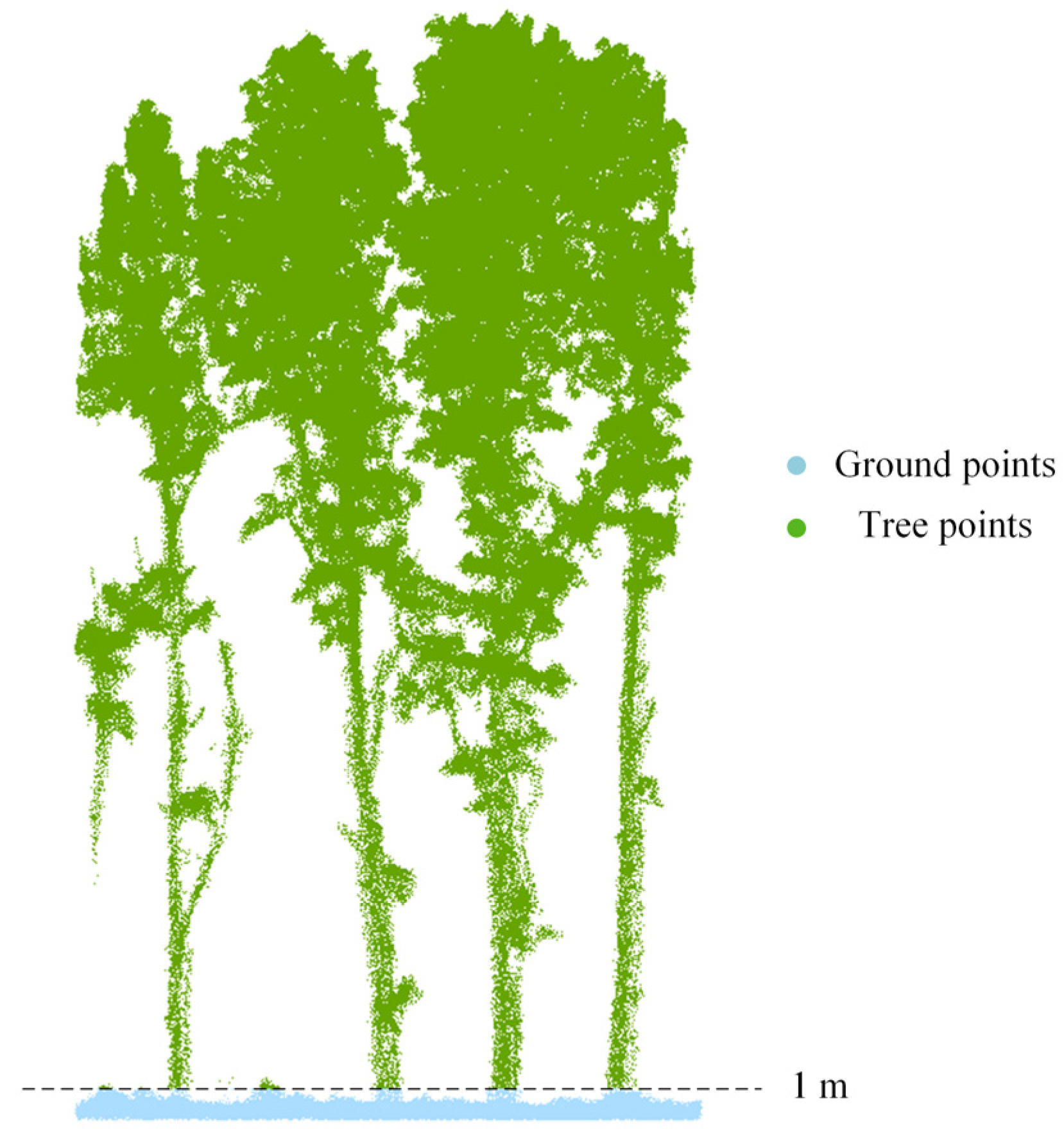
To determine the optimal spatial scale for LAI estimation in the study area, three sampling radii—5 m, 10 m, and 15 m—were applied to the processed LiDAR data, centered on the coordinates of the field-measured LAI plots. A height threshold of 1 m was applied to classify LiDAR points: returns below this threshold were considered ground or low vegetation, while those above were classified as canopy points (Figure 2). This threshold was determined based on field observations and analysis of LiDAR point cloud structure, where all vegetation above 1 m consisted of overstory trees, and herbaceous layers were predominantly below 1 m. Point classification was performed using CloudCompare (v2.13.2).
For each sampling scale, the LiDAR Penetration Index (LPI) was calculated for every sample plot using Equation (1). The LPI is defined as the ratio of ground-classified returns to the total number of returns [14]. In this context, LPI quantifies canopy openness. Ng represents the number of ground or low-vegetation returns (below 1 m), and Nv represents canopy returns (above 1 m).
LPI = N g N g +   N v

2.4. Calculation of Point Cloud Texture Features

In point cloud data analysis, texture features are used to characterize the micro-scale geometric variations of surface structures and are widely applied in vegetation structure assessment, terrain modeling, and object recognition [26]. In this study, three texture features—roughness, curvature, and density—were computed based on tree-classified LiDAR points. All computations were performed using Python 3.9 and the Open3D 0.17.0 library, which offers efficient tools for 3D point cloud manipulation, KDTree search, and normal estimation [14].

2.4.1. Roughness

Roughness describes the irregularity of the surface and is typically inferred from normal vector fluctuations. Normal vectors were estimated using a hybrid KDTree method with a fixed neighborhood search radius of 0.1 m and maximum of 30 neighbors. For each point, the standard deviation of the estimated normals in its local neighborhood was calculated. The global roughness was expressed as the average of these local roughness values across all vegetation points [27]. This feature effectively reflects small-scale canopy surface undulations and has proven useful in vegetation structural analysis [28]. The roughness (R) is expressed as
R = 1 N i = 1 N σ n i
where R is the average roughness of the entire point cloud, N is the total number of points, ni ∈ R3 is the normal vector at point i, and σ (ni) represents the standard deviation of normals in the neighborhood of point i, computed within a fixed radius r.

2.4.2. Curvature

Curvature describes the degree of local geometric deformation of the surface and indicates the extent of bending. In this study, curvature was computed to quantify local geometric bending and structure sharpness. Following the same normal estimation procedure (0.1 m radius, max 30 neighbors), curvature was calculated as the Euclidean norm of the spatial gradient of the normal vectors [29]. Larger curvature values typically correspond to areas with sharp structural changes such as canopy edges or dense foliage regions [30]. The curvature C is expressed as
C = 1 N i = 1 N n i 2
where C is the average curvature, n i is the spatial gradient of the normal vector at point i, and · 2 denotes the Euclidean norm.

2.4.3. Density

Density reflects the degree of point aggregation within a given spatial volume and is an important indicator of point cloud completeness. Point cloud density was measured by counting the number of neighbors within a fixed radius of 0.1 m around each point, using a KDTree radius search. For each vegetation point, the number of neighbors found was recorded and the global density was calculated as their mean [31]. The density D is defined as
D = 1 N i = 1 N k i
where D is the average point cloud density, ki is the number of points within a radius r centered at point i, and N is the total number of points in the dataset.

2.5. Multivariate Linear Regression Model for LAI Estimation Integrating Texture Features and LPI

Indirect estimation of LAI is commonly based on the Beer–Lambert law, which models canopy gap fraction as an exponential function of LAI Equation (3) [32]. In this formulation, LAI represents the leaf area index, I denotes the light transmitted through the canopy, I0 is the incident light above the canopy, and k is the extinction coefficient, which depends on leaf angle distribution and the direction of incoming radiation. When k is known, the LPI reflects the fraction of LiDAR pulses that reach the ground, analogous to the optical gap fraction (I/I0) used in the Beer–Lambert formulation. Several studies have supported the substitution of LiDAR-based metrics for optical gap fraction due to the comparable canopy penetration behavior of near-infrared laser pulses and diffuse sunlight. Therefore, LPI can serve as a structural proxy for canopy openness under the Beer–Lambert model framework, and LAI can be calculated from the ratio I/I0, which essentially corresponds to the canopy gap fraction [14]:
I   =   I 0 · e k · LAI
Recent studies have shown that the inclusion of structural or texture features can significantly improve the accuracy of biophysical parameter estimation [33]. Therefore, in this study, structural texture features are introduced as empirical variables to correct the LPI-based estimation of LAI, compensating for LPI’s limited ability to capture complex canopy structures. Integrating such features within a statistical modeling framework has been demonstrated to be both logical and effective [34,35]. By incorporating the three point cloud texture features—roughness (R), curvature (C), and density (D)—Equation (3) can be reformulated as
I = I 0 · e k 1 · LAI k 2 · R k 3 · C k 4 · D
Substituting the canopy gap fraction with LPI and introducing an intercept term, the empirical expression for estimating LAI from LPI and texture features becomes
LAI i = 1 k ln LPI i + c · R + d · C + e · D + b
where LAIi is the LAI at the i-th sampling point, LPIi is the LiDAR-derived gap fraction at the same location, c, d, and e are the regression coefficients for roughness, curvature, and density, respectively, and b is the intercept term.
Prior to model fitting, all independent variables were tested for potential multicollinearity. To detect redundancy and interdependence among predictors, the Variance Inflation Factor (VIF) was calculated for each variable (LPI, R, C, and D). A VIF value greater than 5 typically indicates moderate to severe multicollinearity.
Since differences in the spectral properties of background and vegetation can introduce bias between the LPI and true canopy gap fraction—and this discrepancy increases as spectral contrast becomes greater. Previous studies have proposed a calibration method for LPI Equation (6). The adjusted LPI (LPIadj) can be calculated using one of three approaches: (1) deriving the correction factor μ from ground-based or hyperspectral remote sensing data [36,37]; (2) empirically testing a range of μ values to identify the one that yields the highest coefficient of determination (R2) between predicted and observed LAI [38]; or (3) estimating μ from LiDAR return intensity [39]. As spectral data were unavailable in this study and return intensity could not reliably isolate spectral effects, the second method was adopted to determine the optimal μ.
LPI adj = LPI μ + 1 + μ LPI

3. Results

3.1. Optimal Adjustment Coefficient for LPI

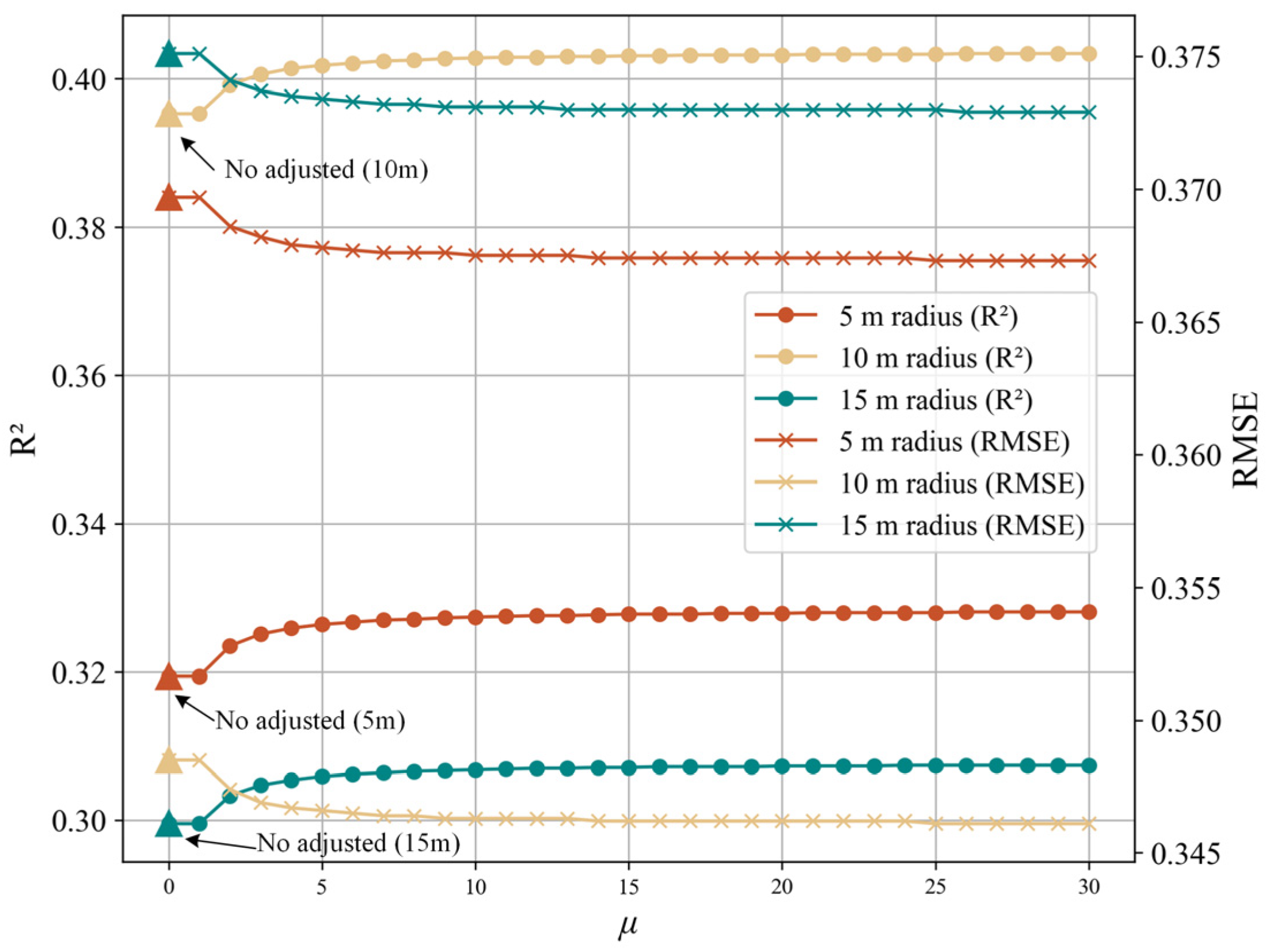
To enhance the correlation between the LiDAR Penetration Index (LPI) and the Leaf Area Index (LAI), an adjustment coefficient μ was introduced to calibrate the original LPI values. The coefficient was varied incrementally from 0 to 30 with a step size of 1. Figure 3 illustrates the variation of the coefficient of determination (R2) and Root Mean Square Error (RMSE) for LAI regression models using LPI alone at three spatial scales (buffer radii of 5 m, 10 m, and 15 m) under different values of μ.
As shown in the figure, the R2 values at all three spatial scales initially increased with rising μ, followed by a rapid plateauing trend. This indicates that appropriate adjustment can significantly enhance the correlation between the penetration index and observed LAI. For example, at the 10 m buffer radius, R2 improved from 0.3953 (unadjusted) to 0.4031 when μ = 15; beyond this point, further increases in μ yielded only marginal improvement, reaching 0.4034, suggesting diminishing returns. Similarly, RMSE decreased rapidly with small increases in μ but also plateaued at higher values. Considering both performance gain and parameter simplicity, μ = 15 was ultimately selected as the optimal adjustment coefficient. This value achieves near-maximum model performance across spatial scales while avoiding potential overfitting or dilution of physical interpretability.

3.2. LAI Estimation Accuracy Using LPI at Different Spatial Scales

To evaluate the effect of spatial scale, circular extraction windows with radii of 5 m, 10 m, and 15 m were used to extract LiDAR point cloud data. LPI was calculated for each spatial scale and regressed against 40 ground-measured LAI samples. Table 1 summarizes the performance of the LAI estimation models based on LPI at the three scales.
From Table 1, it can be concluded that a 10 m extraction radius yields the best performance for LAI estimation in the study area. The highest accuracy was achieved using the echo-based LPI model at this scale (R2 = 0.40, RMSE = 0.35). After adjustment, the logarithmic transformation of LPI, i.e., −ln(LPI), showed strong correlation with observed LAI (R2 > 0.4), as shown in Figure 4.
To further evaluate whether the observed differences in model performance across scales were statistically significant, we conducted a Kruskal–Wallis H test on the residual errors due to the non-normal distribution of residuals (Shapiro–Wilk test, p < 0.05). Results showed a statistically significant difference in model accuracy across spatial scales (p < 0.01), with the 10 m scale outperforming the others. In addition, we assessed whether the assumption of linearity and homoscedasticity between observed LAI and −ln(LPI) held true using residual scatterplots and Breusch–Pagan tests. The residuals exhibited no strong heteroscedasticity (p > 0.05), supporting the suitability of the linear model structure across all scales.

3.3. LAI Estimation Incorporating Texture Features

A multivariate regression model was constructed using the optimally adjusted LPI (μ = 15) and point cloud-derived texture features. The model used field-measured LAI as the dependent variable, with −ln(LPI), roughness (R), curvature (C), and density (D) as predictors. Table 2 presents the regression results before and after the incorporation of texture features.
As shown in Table 2, the VIF values for LPI_ground_adj_mu_15 and Average Roughness are relatively low, indicating weak multicollinearity between them. However, the VIF values for Average Curvature and Average Density are higher, particularly for Average Density, which has a VIF close to 28, suggesting significant multicollinearity with other variables. According to VIF standards (where values greater than 5 generally indicate multicollinearity), we decided to remove the density variable from the model. After its removal, multicollinearity in the model was significantly reduced, and the VIF values became more reasonable. The removal of density is justified because it was highly correlated with other variables, contributed weakly to LAI estimation, and its removal did not significantly affect the model’s explanatory power.
Next, we present the complete regression results, which include coefficients, standard errors, p-values, RMSE, R2, MAE, and AIC values. These results offer a comprehensive reflection of the model’s performance.
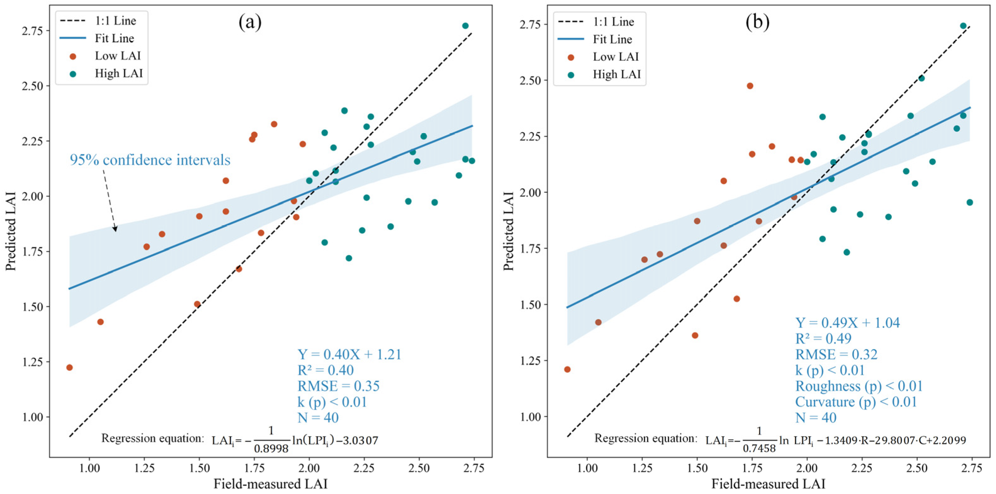
The regression analysis yielded two predictive models. For LPI alone, the regression equation is LAI i   =   - 1 0.8998 ln LPI i   -   3 . 0307 (p < 0.01). When incorporating texture features (roughness and curvature), the multivariate regression equation becomes LAI i   =   - 1 0.7458 ln LPI i   -   1.3409 · R   -   29.8007 · C   +   2.2099 .
Table 3 presents the regression results for the multivariate model incorporating texture features. All regression coefficients (k, c, and d) are statistically significant with p-values < 0.01, indicating strong statistical significance for both the LPI-only model and the multivariate model with texture features. The multivariate regression model demonstrates that the combination of LPI, roughness, and curvature provides improved prediction for LAI. The R2 value of 0.49 suggests that the model explains nearly 50% of the variability in LAI, compared to the LPI-only model. The RMSE value of 0.32 indicates that the model’s prediction error is relatively small, while the MAE value of 0.26 further indicates minimal prediction bias. The AIC value of 30.68 suggests that the model achieves a reasonable balance between fitting accuracy and complexity.
Furthermore, we performed a 10-fold cross-validation to assess the generalizability and robustness of the model. The average R2 and RMSE values from the cross-validation were 0.47 and 0.33, respectively, which closely align with the model’s performance on the training set, supporting the stability of the model and its ability to generalize to unseen data (Figure 5).
In conclusion, the multivariate regression model incorporating texture features (roughness and curvature) showed improvement in LAI estimation accuracy compared to the LPI-only approach. All coefficients in both models were statistically significant (p < 0.01), demonstrating the reliability of the predictive relationships. The cross-validation results further confirm the model’s robustness and generalizability. Compared to LPI alone, the model incorporating texture features showed moderate improvement, highlighting the potential value of texture features in enhancing LAI prediction capabilities.

4. Discussion

4.1. Limitations of LAI Estimation Using LPI

The fundamental principle of the LPI is to estimate canopy gap fraction indirectly by calculating the ratio of laser returns reaching the ground to the total number of returns, and then deriving LAI via the Beer–Lambert Law. In this study, although an adjustment coefficient of μ = 15 was applied to calibrate LPI and the 10 m scale achieved optimal fitting accuracy, the performance of LPI-based LAI estimation remained moderate. Below are quantitative limitations observed in our context.
Despite high point density in UAV-based LiDAR, laser penetration is significantly constrained in dense forest mid- and upper canopy layers. For instance, in tropical forests with dense foliage, only 10%–30% of LiDAR pulses typically reach the ground, resulting in reduced ground return counts and underestimation of gap fraction [40,41]. Moreover, studies have shown that when canopy density increases, LPI-based gap fraction estimates can be biased by 10%–20%, and corresponding LAI estimates become inflated by a similar margin [42]. Point density and scan angle also contribute to precision loss. Quantitative analyses indicate that below a critical density threshold (e.g., <10 pts/m2 in ALS data), structural canopy metrics, including gap fraction and LAI, become increasingly unreliable [43]. These effects are exacerbated at steep scan angles or high divergence, where canopy occlusion increases ground return loss. Collectively, these factors explain why LPI alone struggles in structurally complex or dense canopy environments and underlines the benefit of integrating additional texture-based features.

4.2. Scientific Justification for Using Texture Features to Enhance LPI-Based LAI Estimation

Among various LiDAR-based LAI estimation methods, the LPI remains a fundamental structural metric. It effectively reflects canopy gap fraction and exhibits an exponential decay relationship with the LAI [20]. However, as a single return-based indicator, LPI does not capture the full structural complexity of multilayered, heterogeneous vegetation canopies, often leading to reduced estimation accuracy [44]. To enhance model robustness and predictive power, it is necessary to integrate additional descriptors that characterize 3D canopy structure more comprehensively.
Point cloud texture features derived from 3D LiDAR data provide valuable insights into the local geometric variations of canopy surfaces. In vegetated areas, roughness characterizes surface irregularity and is sensitive to the spatial distribution of leaves and leaf clumping, which directly influences light penetration and LAI [45]. Curvature, representing the deviation of local surfaces from planarity, has been found to reflect structural properties such as branch bending and leaf orientation, which relate to canopy complexity and functional traits [46,47].
Initially, point density was considered as an additional texture feature, serving as a proxy for local foliage concentration and biomass, which affects both occlusion and laser return distribution [48]. However, our analysis revealed high multicollinearity between density and other variables (VIF = 28.05), necessitating its removal from the final model. This strong correlation can be attributed to the inherent relationship between point density and canopy structural properties: dense canopies naturally generate more LiDAR returns due to increased surface area and multiple scattering events, creating redundancy with LPI measurements [49]. Additionally, point density is often correlated with surface roughness in vegetation canopies, as structurally complex areas tend to produce higher return densities [50].
The final model incorporating roughness and curvature alongside LPI enables a richer representation of canopy heterogeneity than a single structural index alone, while avoiding the statistical complications of multicollinearity. Previous studies that included textural metrics such as roughness alongside penetration-based indices have demonstrated improved performance in vegetation classification and leaf area estimation [43]. The complementary nature of these features—with LPI capturing vertical structure, roughness characterizing surface complexity, and curvature reflecting geometric irregularities—provides a more comprehensive description of canopy architecture without redundant information.
From a statistical modeling perspective, employing a multivariate linear regression framework to combine LPI with the selected texture features allows LPI to serve as the core explanatory variable, while roughness and curvature are introduced in a linear form to enhance model flexibility and structural adaptability. This approach adheres to the core principles of optical theory while leveraging orthogonal structural descriptors to capture canopy heterogeneity, aligning with current trends in LiDAR-based remote sensing modeling [37].

4.3. Adaptability Analysis of Multi-Scale Modeling Strategy

This study adopted three different spatial scales for analysis. The results showed that the model performed best at the 10 m scale, suggesting that this observation scale achieved the optimal balance between LiDAR point density, canopy structural features, and sampling resolution within the study area.
The selection of spatial scale is critical for balancing structural detail and model stability. Smaller windows such as 5 m, while sensitive to fine-scale canopy variability, are more susceptible to noise from undergrowth, terrain, and scanning angle artifacts. Larger windows like 15 m tend to over-smooth heterogeneity and dilute local structural patterns, reducing model responsiveness. The 10 m radius likely aligns with the mean canopy height in the study area, consistent with previous studies recommending that sampling radius be approximately 75%–100% of canopy height to capture representative structural attributes [14]. This scale not only improves signal-to-noise ratio but also enhances robustness to intra-plot variation by averaging sub-canopy differences.
However, the optimal spatial scale may vary across ecosystems. In deciduous or mixed-species forests with taller or more layered canopies, larger windows might be necessary to capture vertical complexity. Similarly, in sparse or shrub-dominated systems, smaller scales may be more appropriate. A recent study further confirmed that the effectiveness of scale selection is highly dependent on terrain, canopy structure, and LiDAR acquisition parameters such as flight altitude and scan angle. Their research in montane broadleaf forests showed that point density and directional scanning patterns significantly affected LAI estimation accuracy at different scales, highlighting the need for adaptive, context-specific spatial strategies [51].
Thus, while 10 m performed best in our context, it should be viewed as a contextual optimum, and scale selection should be calibrated based on canopy structure, LiDAR sensor specifications, and research objectives in future applications. Moreover, scale variations also affect model stability and sensitivity. Smaller sampling radii may increase sensitivity to local heterogeneity, reducing model robustness. Conversely, larger sampling scales may over-smooth local structural features, leading to diminished estimation accuracy [52]. Therefore, selecting an appropriate sampling scale is critical to capturing sufficient structural information while maintaining model stability.

4.4. Model Enhancement and Future Research Directions

While the integration of LPI and texture features demonstrates promising results in this study, several limitations constrain the model’s generalizability and accuracy. The current analysis is based on a relatively small dataset within a homogeneous poplar plantation. This restricts the model’s robustness, especially when applied to more diverse or structurally complex forest types.
In future research, integrating additional data sources such as spectral information may offer significant advantages. Specifically, multispectral and hyperspectral sensors mounted on UAV platforms can provide canopy reflectance and biochemical characteristics (e.g., chlorophyll and moisture content), which are complementary to structural data [53]. Thermal infrared imaging can further assist in capturing plant water stress and evapotranspiration dynamics [54]. These spectral cues could help reduce the estimation bias observed in high or low LAI ranges.
Moreover, the use of advanced nonlinear models, such as Random Forest (RF) and Convolutional Neural Networks (CNNs), can better capture complex interactions between structural and spectral features [55,56]. Random Forests are especially advantageous due to their resistance to overfitting and their ability to quantify variable importance, while CNNs are well-suited to analyzing 3D voxel representations or hyperspectral cubes. Hybrid ensemble models may also be explored to integrate multiple algorithms and enhance model generalization across forest types.

5. Conclusions

This study focused on the Shishou National Poplar Breeding Base as the experimental area and systematically investigated the feasibility and adaptability of combining UAV LiDAR point cloud data with visible imagery to estimate LAI using LPI and VDVI across multiple spatial scales. A multi-source remote sensing framework suitable for LAI estimation under conditions lacking near-infrared information was developed, and the following main conclusions were drawn:
(1) The LPI effectively captured canopy gap characteristics and exhibited a strong correlation with field-measured LAI, particularly when calibrated using a correction coefficient (μ = 15). However, due to structural limitations in complex and multilayered canopies, LPI alone could not fully represent foliage distribution. By incorporating texture features such as roughness and curvature, the model better accounted for canopy heterogeneity, significantly enhancing LAI estimation accuracy. This integration demonstrates the compensatory effect of local structural descriptors in addressing the intrinsic limitations of return-based indices like LPI.
(2) Among the tested spatial scales, the 10 m resolution achieved the most balanced performance by integrating sufficient point cloud density and representative canopy structure. Both finer (5 m) and coarser (15 m) scales showed reduced model robustness, indicating the critical role of spatial scale in LAI modeling.
(3) Future research should focus on expanding the model across more diverse forest types and ecological conditions. Specifically, the incorporation of high-dimensional spectral data (e.g., multispectral, hyperspectral, and thermal imagery), LiDAR intensity, and voxel-based metrics is recommended. In addition, applying nonlinear modeling approaches such as Random Forest or deep learning frameworks may further improve predictive accuracy and generalizability. The integration of multi-temporal UAV data, field sampling, and terrestrial LiDAR will be essential for building robust, transferable LAI estimation models applicable across ecosystems.

Author Contributions

Conceptualization, Z.L. and Y.D.; methodology, Z.L. and Y.D.; software, Z.L. and Z.Z.; validation, Z.L.; formal analysis, Z.L. and Y.D.; investigation, Z.L., Z.Z., S.C. and Z.C.; resources, Y.D., S.C. and Z.C.; data curation, Z.L. and Z.Z.; writing—original draft preparation, Z.L.; writing—review and editing, Y.D.; visualization, Z.L. and Z.Z.; supervision, Y.D.; project administration, Z.L. and Y.D.; funding acquisition, Y.D. All authors have read and agreed to the published version of the manuscript.

Funding

This research was funded by the Biological Breeding-National Science and Technology Major Project, grant number 2023ZD0405605.

Data Availability Statement

The raw data supporting the conclusions of this article will be made available by the authors on request.

Conflicts of Interest

The authors declare no conflicts of interest.

References

  1. Lafont, S.; Zhao, Y.; Calvet, J.-C.; Peylin, P.; Ciais, P.; Maignan, F.; Weiss, M. Modelling LAI, Surface Water and Carbon Fluxes at High-Resolution over France: Comparison of ISBA-A-Gs and ORCHIDEE. Biogeosciences 2012, 9, 439–456. [Google Scholar] [CrossRef]
  2. Chen, J.M.; Ju, W.; Ciais, P.; Viovy, N.; Liu, R.; Liu, Y.; Lu, X. Vegetation Structural Change since 1981 Significantly Enhanced the Terrestrial Carbon Sink. Nat. Commun. 2019, 10, 4259. [Google Scholar] [CrossRef] [PubMed]
  3. Li, Y.; Shi, H.; Zhou, L.; Eamus, D.; Huete, A.; Li, L.; Cleverly, J.; Hu, Z.; Harahap, M.; Yu, Q.; et al. Disentangling Climate and LAI Effects on Seasonal Variability in Water Use Efficiency Across Terrestrial Ecosystems in China. J. Geophys. Res. Bio Geosci. 2018, 123, 2429–2443. [Google Scholar] [CrossRef]
  4. Xu, Y.; Calvet, J.-C.; Bonan, B. The Joint Assimilation of Satellite Observed LAI and Soil Moisture for the Global Root Zone Soil Moisture Production and Its Impact on Land Surface and Ecosystem Variables. Agric. For. Meteorol. 2025, 360, 110299. [Google Scholar] [CrossRef]
  5. Cordak, A.S.; Kooperman, G.J.; Zarakas, C.M.; Swann, A.L.S.; Koven, C.D. The Role of Leaf Area Changes Within Plant CO2 Physiological Impacts on the Global Hydrological Cycle. Geophys. Res. Lett. 2025, 52, e2024GL110904. [Google Scholar] [CrossRef]
  6. Huang, S.; Tang, L.; Hupy, J.P.; Wang, Y.; Shao, G. A Commentary Review on the Use of Normalized Difference Vegetation Index (NDVI) in the Era of Popular Remote Sensing. J. For. Res. 2021, 32, 1–6. [Google Scholar] [CrossRef]
  7. Huete, A.; Didan, K.; van Leeuwen, W.; Miura, T.; Glenn, E. MODIS Vegetation Indices. In Land Remote Sensing and Global Environmental Change: NASA’s Earth Observing System and the Science of ASTER and MODIS; Ramachandran, B., Justice, C.O., Abrams, M.J., Eds.; Springer: New York, NY, USA, 2011; pp. 579–602. ISBN 978-1-4419-6749-7. [Google Scholar]
  8. Chen, J.M.; Cihlar, J. Retrieving Leaf Area Index of Boreal Conifer Forests Using Landsat TM Images. Remote Sens. Environ. 1996, 55, 153–162. [Google Scholar] [CrossRef]
  9. Martinez, A.D.L.I.; Labib, S.M. Demystifying Normalized Difference Vegetation Index (NDVI) for Greenness Exposure Assessments and Policy Interventions in Urban Greening. Environ. Res. 2023, 220, 115155. [Google Scholar] [CrossRef]
  10. Huete, A.; Didan, K.; Miura, T.; Rodriguez, E.P.; Gao, X.; Ferreira, L.G. Overview of the Radiometric and Biophysical Performance of the MODIS Vegetation Indices. Remote Sens. Environ. 2002, 83, 195–213. [Google Scholar] [CrossRef]
  11. Grigorov, B. An Investigation of The Forests of Pernik Province (Western Bulgaria) by the Use of The Perpendicular Vegetation Index (PVI). Civ. Environ. Eng. Rep. 2022, 32, 96–104. [Google Scholar] [CrossRef]
  12. Pamungkas, S. Analysis of Vegetation Index for Ndvi, Evi-2, And Savi For Mangrove Forest Density Using Google Earth Engine In Lembar Bay, Lombok Island. IOP Conf. Ser. Earth Environ. Sci. 2023, 1127, 012034. [Google Scholar] [CrossRef]
  13. Lefsky, M.A.; Cohen, W.B.; Parker, G.G.; Harding, D.J. Lidar Remote Sensing for Ecosystem Studies: Lidar, an Emerging Remote Sensing Technology That Directly Measures the Three-Dimensional Distribution of Plant Canopies, Can Accurately Estimate Vegetation Structural Attributes and Should Be of Particular Interest to Forest, Landscape, and Global Ecologists. BioScience 2002, 52, 19–30. [Google Scholar] [CrossRef]
  14. Wang, Y.; Fang, H. Estimation of LAI with the LiDAR Technology: A Review. Remote Sens. 2020, 12, 3457. [Google Scholar] [CrossRef]
  15. Simard, M.; Pinto, N.; Fisher, J.B.; Baccini, A. Mapping Forest Canopy Height Globally with Spaceborne Lidar. J. Geophys. Res. Bio Geosci. 2011, 116. [Google Scholar] [CrossRef]
  16. Zhu, X.; Liu, J.; Skidmore, A.K.; Premier, J.; Heurich, M. A Voxel Matching Method for Effective Leaf Area Index Estimation in Temperate Deciduous Forests from Leaf-on and Leaf-off Airborne LiDAR Data. Remote Sens. Environ. 2020, 240, 111696. [Google Scholar] [CrossRef]
  17. Su, W.; Huang, J.; Liu, D.; Zhang, M. Retrieving Corn Canopy Leaf Area Index from Multitemporal Landsat Imagery and Terrestrial LiDAR Data. Remote Sens. 2019, 11, 572. [Google Scholar] [CrossRef]
  18. Zheng, G.; Moskal, L.M. Retrieving Leaf Area Index (LAI) Using Remote Sensing: Theories, Methods and Sensors. Sensors 2009, 9, 2719–2745. [Google Scholar] [CrossRef] [PubMed]
  19. Duan, S.-B.; Li, Z.-L.; Wu, H.; Tang, B.-H.; Ma, L.; Zhao, E.; Li, C. Inversion of the PROSAIL Model to Estimate Leaf Area Index of Maize, Potato, and Sunflower Fields from Unmanned Aerial Vehicle Hyperspectral Data. Int. J. Appl. Earth Obs. Geoinf. 2014, 26, 12–20. [Google Scholar] [CrossRef]
  20. Luo, S.-Z.; Wang, C.; Zhang, G.-B.; Xi, X.-H.; Li, G.-C. Forest Leaf Area Index (LAI) Estimation Using Airborne Discrete-Return Lidar Data. Chin. J. Geophys. 2013, 56, 233–242. [Google Scholar] [CrossRef]
  21. Saitoh, T.M.; Nagai, S.; Noda Hibiki, M.; Muraoka, H.; Nasahara, K.N. Examination of the Extinction Coefficient in the Beer–Lambert Law for an Accurate Estimation of the Forest Canopy Leaf Area Index. For. Sci. Technol. 2012, 8, 67–76. [Google Scholar] [CrossRef]
  22. Tan, K.; Ke, T.; Tao, P.; Liu, K.; Duan, Y.; Zhang, W.; Wu, S. Discriminating Forest Leaf and Wood Components in TLS Point Clouds at Single-Scan Level Using Derived Geometric Quantities. IEEE Trans. Geosci. Remote Sens. 2022, 60, 1–17. [Google Scholar] [CrossRef]
  23. Wang, Y.; Gu, Y.; Tang, J.; Guo, B.; Warner, T.A.; Guo, C.; Zheng, H.; Hosoi, F.; Cheng, T.; Zhu, Y.; et al. Quantify Wheat Canopy Leaf Angle Distribution Using Terrestrial Laser Scanning Data. IEEE Trans. Geosci. Remote Sens. 2024, 62, 1–15. [Google Scholar] [CrossRef]
  24. Zhang, Y.; Han, X.; Yang, J. Exploring the Performance of Spectral and Textural Information for Leaf Area Index Estimation with Homogeneous and Heterogeneous Surfaces. Photogramm. Rec. 2023, 38, 233–251. [Google Scholar] [CrossRef]
  25. Wang, C.; Luo, S.; Xi, X.; Nie, S.; Ma, D.; Huang, Y. Influence of Voxel Size on Forest Canopy Height Estimates Using Full-Waveform Airborne LiDAR Data. For. Ecosyst. 2020, 7, 31. [Google Scholar] [CrossRef]
  26. Lai, X.; Yang, J.; Li, Y.; Wang, M. A Building Extraction Approach Based on the Fusion of LiDAR Point Cloud and Elevation Map Texture Features. Remote Sens. 2019, 11, 1636. [Google Scholar] [CrossRef]
  27. Brodu, N.; Lague, D. 3D Terrestrial Lidar Data Classification of Complex Natural Scenes Using a Multi-Scale Dimensionality Criterion: Applications in Geomorphology. ISPRS J. Photogramm. Remote Sens. 2012, 68, 121–134. [Google Scholar] [CrossRef]
  28. Fan, L. Comparisons of Five Indices for Estimating Local Terrain Surface Roughness Using LiDAR Point Clouds. In Proceedings of the 2022 29th International Conference on Geoinformatics, Beijing, China, 15 August 2022; pp. 1–6. [Google Scholar]
  29. Bischoff, S.; Kobbelt, L. Sub-Voxel Topology Control for Level-Set Surfaces. Comput. Graph. Forum 2003, 22, 273–280. [Google Scholar] [CrossRef]
  30. Lindberg, E.; Holmgren, J. Individual Tree Crown Methods for 3D Data from Remote Sensing. Curr. For. Rep. 2017, 3, 19–31. [Google Scholar] [CrossRef]
  31. Hackel, T.; Wegner, J.D.; Schindler, K. Fast Semantic Segmentation of 3D Point Clouds with Strongly Varying Density. ISPRS Ann. Photogramm. Remote Sens. Spat. Inf. Sci. 2016, III-3, 177–184. [Google Scholar] [CrossRef]
  32. Tan, C.-W.; Zhang, P.-P.; Zhou, X.-X.; Wang, Z.-X.; Xu, Z.-Q.; Mao, W.; Li, W.-X.; Huo, Z.-Y.; Guo, W.-S.; Yun, F. Quantitative Monitoring of Leaf Area Index in Wheat of Different Plant Types by Integrating NDVI and Beer-Lambert Law. Sci. Rep. 2020, 10, 929. [Google Scholar] [CrossRef]
  33. Kukkonen, M.; Lähivaara, T.; Packalen, P. Combination of Lidar Intensity and Texture Features Enable Accurate Prediction of Common Boreal Tree Species with Single Sensor UAS Data. IEEE Trans. Geosci. Remote Sens. 2024, 62, 1–8. [Google Scholar] [CrossRef]
  34. García, M.; Riaño, D.; Chuvieco, E.; Salas, J.; Danson, F.M. Multispectral and LiDAR Data Fusion for Fuel Type Mapping Using Support Vector Machine and Decision Rules. Remote Sens. Environ. 2011, 115, 1369–1379. [Google Scholar] [CrossRef]
  35. Jakovljevic, G.; Govedarica, M.; Alvarez-Taboada, F. A Deep Learning Model for Automatic Plastic Mapping Using Unmanned Aerial Vehicle (UAV) Data. Remote Sens. 2020, 12, 1515. [Google Scholar] [CrossRef]
  36. Morsdorf, F.; Kötz, B.; Meier, E.; Itten, K.I.; Allgöwer, B. Estimation of LAI and Fractional Cover from Small Footprint Airborne Laser Scanning Data Based on Gap Fraction. Remote Sens. Environ. 2006, 104, 50–61. [Google Scholar] [CrossRef]
  37. Qu, Y.; Shaker, A.; Korhonen, L.; Silva, C.A.; Jia, K.; Tian, L.; Song, J. Direct Estimation of Forest Leaf Area Index Based on Spectrally Corrected Airborne LiDAR Pulse Penetration Ratio. Remote Sens. 2020, 12, 217. [Google Scholar] [CrossRef]
  38. Solberg, S. Mapping Gap Fraction, LAI and Defoliation Using Various ALS Penetration Variables. Int. J. Remote Sens. 2010, 31, 1227–1244. [Google Scholar] [CrossRef]
  39. Armston, J.; Disney, M.; Lewis, P.; Scarth, P.; Phinn, S.; Lucas, R.; Bunting, P.; Goodwin, N. Direct Retrieval of Canopy Gap Probability Using Airborne Waveform Lidar. Remote Sens. Environ. 2013, 134, 24–38. [Google Scholar] [CrossRef]
  40. De Almeida, D.R.A.; Stark, S.C.; Shao, G.; Schietti, J.; Nelson, B.W.; Silva, C.A.; Gorgens, E.B.; Valbuena, R.; de Papa, D.A.; Brancalion, P.H.S. Optimizing the Remote Detection of Tropical Rainforest Structure with Airborne Lidar: Leaf Area Profile Sensitivity to Pulse Density and Spatial Sampling. Remote Sens. 2019, 11, 92. [Google Scholar] [CrossRef]
  41. You, H.; Wang, T.; Skidmore, A.K.; Xing, Y. Quantifying the Effects of Normalisation of Airborne LiDAR Intensity on Coniferous Forest Leaf Area Index Estimations. Remote Sens. 2017, 9, 163. [Google Scholar] [CrossRef]
  42. Vaccari, S.; van Leeuwen, M.; Calders, K.; Coops, N.C.; Herold, M. Bias in Lidar-Based Canopy Gap Fraction Estimates. Remote Sens. Lett. 2013, 4, 391–399. [Google Scholar] [CrossRef]
  43. LaRue, E.A.; Fahey, R.; Fuson, T.L.; Foster, J.R.; Matthes, J.H.; Krause, K.; Hardiman, B.S. Evaluating the Sensitivity of Forest Structural Diversity Characterization to LiDAR Point Density. Ecosphere 2022, 13, e4209. [Google Scholar] [CrossRef]
  44. Wang, Y.; Fang, H.; Zhang, Y.; Li, S.; Pang, Y.; Ma, T.; Li, Y. Retrieval and Validation of Vertical LAI Profile Derived from Airborne and Spaceborne LiDAR Data at a Deciduous Needleleaf Forest Site. GIScience Remote Sens. 2023, 60, 2214987. [Google Scholar] [CrossRef]
  45. Béland, M.; Baldocchi, D.D.; Widlowski, J.-L.; Fournier, R.A.; Verstraete, M.M. On Seeing the Wood from the Leaves and the Role of Voxel Size in Determining Leaf Area Distribution of Forests with Terrestrial LiDAR. Agric. For. Meteorol. 2014, 184, 82–97. [Google Scholar] [CrossRef]
  46. Coops, N.C.; Tompalski, P.; Goodbody, T.R.H.; Queinnec, M.; Luther, J.E.; Bolton, D.K.; White, J.C.; Wulder, M.A.; van Lier, O.R.; Hermosilla, T. Modelling Lidar-Derived Estimates of Forest Attributes over Space and Time: A Review of Approaches and Future Trends. Remote Sens. Environ. 2021, 260, 112477. [Google Scholar] [CrossRef]
  47. Peng, X.; Calders, K.; Terryn, L.; Verbeeck, H. Evaluating Tree Branch Angle Measurements of European Beech Using Terrestrial Laser Scanning. For. Ecosyst. 2025, 12, 100279. [Google Scholar] [CrossRef]
  48. Coops, N.C.; Hilker, T.; Wulder, M.A.; St-Onge, B.; Newnham, G.; Siggins, A.; Trofymow, J.A. (Tony) Estimating Canopy Structure of Douglas-Fir Forest Stands from Discrete-Return LiDAR. Trees 2007, 21, 295–310. [Google Scholar] [CrossRef]
  49. Jakubowski, M.K.; Guo, Q.; Kelly, M. Tradeoffs between Lidar Pulse Density and Forest Measurement Accuracy. Remote Sens. Environ. 2013, 130, 245–253. [Google Scholar] [CrossRef]
  50. Campbell, M.J.; Dennison, P.E.; Butler, B.W. A LiDAR-Based Analysis of the Effects of Slope, Vegetation Density, and Ground Surface Roughness on Travel Rates for Wildland Firefighter Escape Route Mapping. Int. J. Wildland Fire 2017, 26, 884–895. [Google Scholar] [CrossRef]
  51. Li, Y.; Zeng, H.; Xiong, J.; Miao, G. Influence of Topography on UAV LiDAR-Based LAI Estimation in Subtropical Mountainous Secondary Broadleaf Forests. Forests 2024, 15, 17. [Google Scholar] [CrossRef]
  52. Zou, J.; Hou, W.; Chen, L.; Wang, Q.; Zhong, P.; Zuo, Y.; Luo, S.; Leng, P. Evaluating the Impact of Sampling Schemes on Leaf Area Index Measurements from Digital Hemispherical Photography in Larix Principis-Rupprechtii Forest Plots. For. Ecosyst. 2020, 7, 52. [Google Scholar] [CrossRef]
  53. Liu, L.; Coops, N.C.; Aven, N.W.; Pang, Y. Mapping Urban Tree Species Using Integrated Airborne Hyperspectral and LiDAR Remote Sensing Data. Remote Sens. Environ. 2017, 200, 170–182. [Google Scholar] [CrossRef]
  54. Leinonen, I.; Jones, H.G. Combining Thermal and Visible Imagery for Estimating Canopy Temperature and Identifying Plant Stress. J. Exp. Bot. 2004, 55, 1423–1431. [Google Scholar] [CrossRef]
  55. Zhu, X.X.; Tuia, D.; Mou, L.; Xia, G.-S.; Zhang, L.; Xu, F.; Fraundorfer, F. Deep Learning in Remote Sensing: A Review. IEEE Geosci. Remote Sens. Mag. 2017, 5, 8–36. [Google Scholar] [CrossRef]
  56. Belgiu, M.; Drăguţ, L. Random Forest in Remote Sensing: A Review of Applications and Future Directions. ISPRS J. Photogramm. Remote Sens. 2016, 114, 24–31. [Google Scholar] [CrossRef]
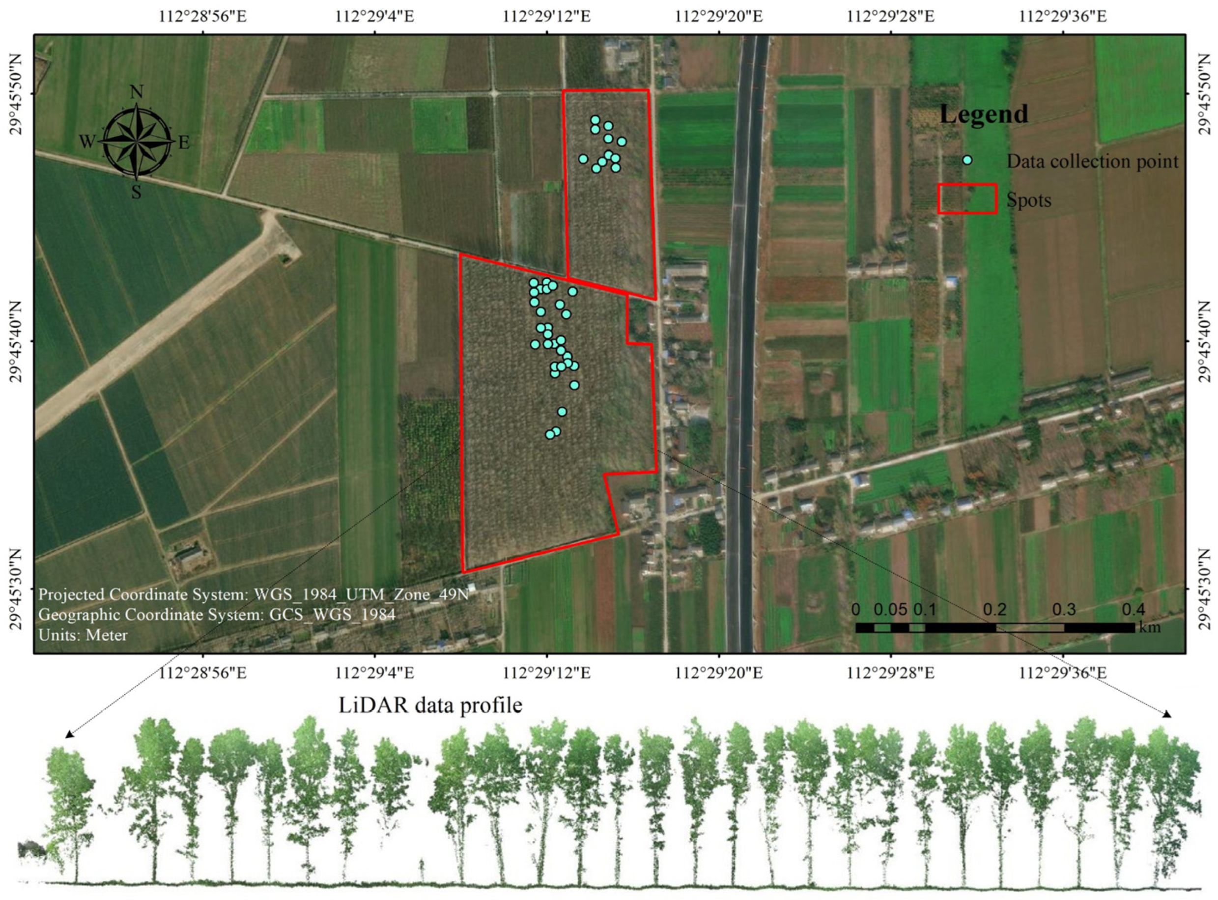
Figure 1. Study area.
Forests 16 01321 g001
Figure 2. Classification of LiDAR returns.
Forests 16 01321 g002
Figure 3. Relationship between LAI estimation accuracy, adjustment coefficient μ, and model performance (R2 and RMSE) across spatial scales.
Forests 16 01321 g003
Figure 4. Regression between measured LAI and −ln(LPI) at three spatial scales: 5 m (a), 10 m (b), and 15 m (c).
Forests 16 01321 g004
Figure 5. Comparison of predicted vs. observed LAI before and after adding texture features: (a) Fitting results of LAI model predictions versus observations without texture features; (b) fitting results of LAI model predictions versus observations with texture features. Marker colors represent LAI value gradients from low (blue) to high (red).
Forests 16 01321 g005
Table 1. Accuracy of LAI estimation using LPI at different spatial scales.
Radius5 m10 m15 m
R20.31940.39530.2995
adjusted R20.32780.40300.3070
RMSE0.36740.34630.3730
Shapiro–Wilk (p)0.01350.02500.0432
Kruskal–Wallis (p)0.0025
Breusch–Pagan (p)0.15350.18250.1256
Table 2. VIF calculation results (comparison before and after removing density).
VariableVIF (Before Removing Density)VIF (After Removing Density)
LPI1.331.18
Roughness1.441.16
Curvature28.481.34
Density28.05-
Table 3. Regression results.
CoefficientValuep-ValueEvaluation IndexValue
k0.7458<0.01RMSE0.32
c−1.3409<0.01R20.49
d−29.8007<0.01MAE0.26
b (Intercept)2.2099/AIC30.68
Disclaimer/Publisher’s Note: The statements, opinions and data contained in all publications are solely those of the individual author(s) and contributor(s) and not of MDPI and/or the editor(s). MDPI and/or the editor(s) disclaim responsibility for any injury to people or property resulting from any ideas, methods, instructions or products referred to in the content.