Article

Research Analysis of the Joint Use of Sentinel-2 and ALOS-2 Data in Fine Classification of Tropical Natural Forests

by
Qingyuan Xie
1,2,3,
Wenxue Fu
1,2,3,*,
Weijun Yan
4,*,
Jiankang Shi
4,
Chengzhi Hao
4,
Hui Li
1,5,
Sheng Xu
6 and
Xinwu Li
1,2,3
1
Key Laboratory of Digital Earth Science, Aerospace Information Research Institute, Chinese Academy of Sciences, Beijing 100094, China
2
International Research Center of Big Data for Sustainable Development Goals, Beijing 100094, China
3
University of Chinese Academy of Sciences, Beijing 100049, China
4
Hainan Provincial Ecological and Environmental Monitoring Centre, Haikou 571126, China
5
Hainan Key Laboratory of Earth Observation, Hainan Aerospace Information Research Institute, Wenchang 571399, China
6
Anhui Ecological and Environment Monitoring Center, Hefei 230071, China
*
Authors to whom correspondence should be addressed.
Forests 2025, 16(8), 1302; https://doi.org/10.3390/f16081302
Submission received: 20 June 2025 / Revised: 23 July 2025 / Accepted: 30 July 2025 / Published: 10 August 2025
(This article belongs to the Section Forest Inventory, Modeling and Remote Sensing)

Abstract

Tropical natural forests play a crucial role in regulating the climate and maintaining global ecosystem functions. However, they face significant challenges due to human activities and climate change. Accurate classification of these forests can help reveal their spatial distribution patterns and support conservation efforts. This study employed four machine learning algorithms—random forest (RF), support vector machine (SVM), Logistic Regression (LR), and Extreme Gradient Boosting (XGBoost)—to classify tropical rainforests, tropical monsoon rainforests, tropical coniferous forests, broadleaf evergreen forests, and mangrove forests on Hainan Island using optical and synthetic aperture radar (SAR) multi-source remote sensing data. Among these, the XGBoost model achieved the best performance, with an overall accuracy of 0.89 and a Kappa coefficient of 0.82. Elevation and red-edge spectral bands were identified as the most important features for classification. Spatial distribution analysis revealed distinct patterns, such as mangrove forests occurring at the lowest elevations and tropical rainforests occupying middle and low elevations. The integration of optical and SAR data significantly enhanced classification accuracy and boundary recognition compared to using optical data alone. These findings underscore the effectiveness of machine learning and multi-source data for tropical forest classification, providing a valuable reference for ecological monitoring and sustainable management.

1. Introduction

Tropical forests are an important part of global terrestrial ecosystems, including natural forests and planted forests, which play a vital role in maintaining the global ecological balance, such as terrestrial carbon cycling [1] and climate regulation [2]. Tropical natural forests are undisturbed or less disturbed ecosystems, which play an indispensable role in maintaining ecological balance; for example, tropical natural forests can protect the soil from erosion [3] and promote the water cycle [4]. Tropical natural forest national parks attract tourists and also bring economic benefits to the local area. In recent years, forest resources in the tropics have faced increasing threats of deforestation and degradation due to human activities [5]. A clear understanding of the spatial distribution of natural forests in the tropics is important for the global carbon cycle, the development of forest resource management strategies, and the reduction in carbon emissions from deforestation and forest degradation [6,7]. Fine classification of tropical natural forests can not only provide a reliable basis for global carbon estimation [8,9], but also support local ecological conservation, in areas such as biodiversity [10], endangered species protection [11], and sustainable management. Under global climate change, the results of fine classification of tropical natural forests can help to assess the impacts of climate change on tropical forests [12] and provide scientific support for global ecology.
Tropical forests are structurally complex and highly forested, and traditional field surveys are inefficient and costly, making it difficult to meet the needs of forest monitoring at large scales and with high timeliness [13]. Remote sensing detection technology has become an effective tool for objectively and realistically monitoring forests over large areas based on the advantages of high timeliness and rich spectral information, and has been widely applied to research in the field of forest monitoring and classification [14]. Nowadays, there are more and more types and quantities of remote sensing image data. It is often difficult to fully capture the spectral characteristics and spatial information of acquired forests from a single data source, e.g., synthetic aperture radar (SAR) imagery is poorly interpretable and is susceptible to corruption with more noise in the data [15], while optical imagery relies on sunlight reflected from objects and is susceptible to weather and cloud cover. The fusion of multispectral data and SAR data can effectively compensate for this deficiency, and image fusion is used to improve the image quality that can be obtained by a single sensor [16], which is enriched with spatial and spectral information, and thus improves the accuracy of forest classification. The synergistic application of multispectral imagery and SAR provides new ideas for this challenge. In recent years, multispectral imagery and SAR imagery have received much attention in forest type classification studies, and Kai et al. [17] and Dino et al. [18] utilized Sentinel-1 and Sentinel-2 data for forest cover monitoring, demonstrating better and more competitive classification accuracy of optical and SAR data fusion and effectiveness in large-scale land cover classification. Optical images are sensors that passively receive a portion of the sunlight reflected from an object, and multispectral images are rich in spectral information, covering the visible and infrared parts [19], and can be distinguished according to the spectral characteristics of different forest types. SAR imagery, on the other hand, involves sensors actively using microwave bands to irradiate vegetation types and record the return energy associated with aboveground biomass and structure [15], where the surface roughness, moisture content, and dielectric properties of various types of objects determine the backscattered energy of each type of object, which in turn helps identify the different objects in the image. A recognized advantage of microwaves is that they are not affected by clouds and weather; especially the longer radar wavelength L-band SAR is better suited for depicting forests than other wavelengths because the main scatters in the L-band are tree branches and canopies, and its penetration into the canopy is stronger, allowing for a more accurate differentiation between forested and non-forested areas [20]. Balling et al. [21] evaluated the potential of ALOS-2 PALSAR-2 ScanSAR (L-band) and Sentinel-1 (C-band) data for tropical forest disturbance mapping, using the island of Sumatra, Indonesia, as a case area. Combining the two sensors produced an 11.9% improvement in accuracy compared to a single sensor. Joshi et al. [22] reviewed 112 related studies on the fusion of multispectral and SAR imagery, which complement each other to achieve more accurate classification mapping. Balling et al. [23] monitored forest disturbance based on dense optical and radar data, and the combined use of sensors improved the accuracy by an average of about 7%. Fan et al. [24] proposed a multi-level interactive fusion network (MLIF-AL) based on adversarial learning, which fully utilized hyperspectral and lidar data through crossmodal interactive information extraction and multi-level feature fusion, and provided a solution for the joint classification of multimodal remote sensing data. Zhu et al. [25] proposed a spectral temporal feature selection (STFS) method based on a weighted separation index (WSI) using multi-temporal Sentinel-2 data to classify tropical forests in the Jianfengling area of Hainan Island. Although the synergistic application of multispectral remote sensing data and SAR data has demonstrated significant potential, there are still notable limitations in the existing research on ecosystem classification of tropical natural forests, both in terms of the limitations of the study scale and the uniqueness of the forest cover type, and in terms of the optimization of classification algorithms and the improvement of the adaptability of the model architecture, and other key issues that are not yet fully addressed. Therefore, there is an urgent need to systematically study the efficacy of multidimensional data combinations and quantitatively compare the results, to provide a theoretical basis and technical support for the accurate identification of complex tropical forest types.
With the development of technology, machine learning methods have become widely used in the field of forest classification. Persson et al. [26] used a random forest classifier based on multi-temporal Sentinel-2 multispectral data to classify five types of tree species in central Sweden, with an overall classification accuracy of 88.2%. Ye et al. [27] integrated PlanetScope with Sentinel-2 using support vector machines, random forests, and neural networks to classify New Zealand native forests, with a maximum accuracy of 95.6%, indicating that the integrated image classification has a higher accuracy than a single classification. In summary, machine learning algorithms have demonstrated high accuracy in tropical natural forest extraction, but there is still no accurate conclusion about the optimal algorithm, especially for the classification research of tropical natural forests. Moreover, the deep learning semantic segmentation approach is currently used to a certain extent in urban tree species extraction [28] and single wood segmentation [29]. However, it usually focuses on airborne high-resolution images or a single simple tree species classification [30], and the approach relies on manually outlined samples, while for natural forests there is a lack of publicly available datasets. Due to the diverse and mixed forest types on Hainan Island, it is difficult to obtain accurate information on the distribution boundaries of natural forests. Therefore, in this study, we developed a dataset suitable for machine learning algorithms based on field survey sampling point data of natural and planted forests, and further compared random forest (RF), support vector machine (SVM), Logistic Regression (LR), and Extreme Gradient Boosting (XGBoost) algorithms in the classification of tropical natural forests.
In view of the complexity and challenges of tropical natural forest classification, this study fully utilized Sentinel-2 multispectral data and ALOS-2 PALSAR synthetic aperture radar data, combined with SRTM DEM data, to construct a dataset adapted to complex tropical natural forest scenes and improve the accuracy of fine classification of tropical natural forests. By systematically comparing four classic machine learning algorithms, RF, SVM, LR, and XGBoost, we explored their applicability and the advantages and disadvantages in tropical natural forest classification. We deeply analyzed the cloudy climate conditions, complex forest structure, and terrain characteristics of Hainan Island, made full use of the ability of L-band data to penetrate the forest canopy, designed and extracted geographical features, spectral features, radar polarization, and backscattering features, and established a natural forest classification system suitable for tropical regions. At the same time, the key factors affecting the spatial distribution of forest types were analyzed, especially the contribution of elevation to the distribution of forest types. This study provides a scientific decision-making basis for the fine classification and sustainable management of tropical natural forests. In addition, future research will try to introduce deep learning methods (e.g., convolutional neural networks, CNNs) in combination with high-resolution remote sensing images to further improve the classification accuracy and model applicability.

2. Materials and Methods

2.1. Study Area

Hainan Island is located at the southern tip of China, and is the second largest island in China, with geographic coordinates between 18°10′ N and 20°10′ N, and between 108°37′ E and 111°03′ E. The topography of Hainan Island is complex, dominated by low mountains, hills, and tablelands, with mountain ranges such as Wuzhishan and Jianfengling in the center, and the terrain gradually decreases from the center to the surroundings [31], as shown in Figure 1. The rivers of Hainan Island are radial water systems, radiating outward from the central mountains or hills and flowing into the South China Sea towards the periphery, and the rich network of water systems and numerous rivers give the region diverse hydrological characteristics [32].
Hainan Island is in a tropical monsoon climate zone, with an average annual temperature of about 24 °C and abundant precipitation, averaging between 1500 and 2500 mm per year, with precipitation concentrated during the summer typhoon and monsoon seasons, which often result in heavy rainfall events. Its climate is characterized by high temperatures and heavy rainfall, the seasons are significantly influenced by the monsoons and typhoons, and the climate type is obvious, with the year divided into two seasons: dry and wet. In the winter half of the year (November to April), under the influence of the northeast monsoon, there is less precipitation, the weather is dry, and the temperature is mild; in the summer half of the year (May to October), under the influence of the southwest monsoon, the precipitation is concentrated, and the weather is hot and humid, forming the wet season [33].
Hainan Island is one of the richest regions in China in terms of tropical forest resources. Hainan’s forest types are diverse, covering a wide range of ecosystems such as typical tropical rainforest, tropical monsoon rainforest, and coastal protection forest. Among them, the typical tropical rainforest is the most representative vegetation type, which is widely distributed in the central and southern mountainous areas, with national nature reserves such as Wuzhishan Mountain and Jianfengling as the core [34].

2.2. Source of Data

In this study, Sentinel-2 data, ALOS-2 PALSAR data, SRTM DEM, and field survey multi-source data (Table 1) were combined to construct a multidimensional feature characterization framework containing spectral features, backscattering features, texture features, and topographic features.
The Sentinel-2 mission, as a core component of the EU Copernicus Earth Observation Program (CEOP), operates in a dual-satellite network mode (Sentinel 2A and 2B) and carries the Multispectral Imager (MSI). Through the synergistic design of orbital phases, the binary star system shortens the 10-day revisit period of a single star to 5 days (equatorial region), realizing global high-frequency observation coverage [35]. The MSI sensor has a 290 km bandwidth covering 13 spectral bands from the visible to the short-wave infrared (SWIR, 443–2190 nm), with spatial resolutions of 10, 20, and 60 m, respectively.
ALOS-2 (Advanced Land Observing Satellite-2) [36] is a second-generation land observation satellite launched by the Japan Aerospace Exploration Agency (JAXA), carrying a PALSAR-2 SAR, with an imaging width ranging from 25 km to 350 km, and a revisit period of 14 days for a single satellite. The satellite operates in the L-band, with a center wavelength of 23.6 cm. The working modes include high-resolution mode, scanning SAR mode, beam scanning mode, etc. According to the different modes, the spatial resolution is also different. In this study, fine-beam dual-polarization data (HH and HV polarization) were acquired for the stripmap mode of ALOS-2 PALSAR in 2022.
This study was based on the Google Earth Engine (GEE) cloud platform to obtain elevation topography data in the Hainan Island area. The SRTM Version 3 Global Digital Elevation Model (Shuttle Radar Topography Mission, SRTM GL1 003, with a spatial resolution of 30 m) jointly released by NASA and NGA was used as the base dataset for the study.
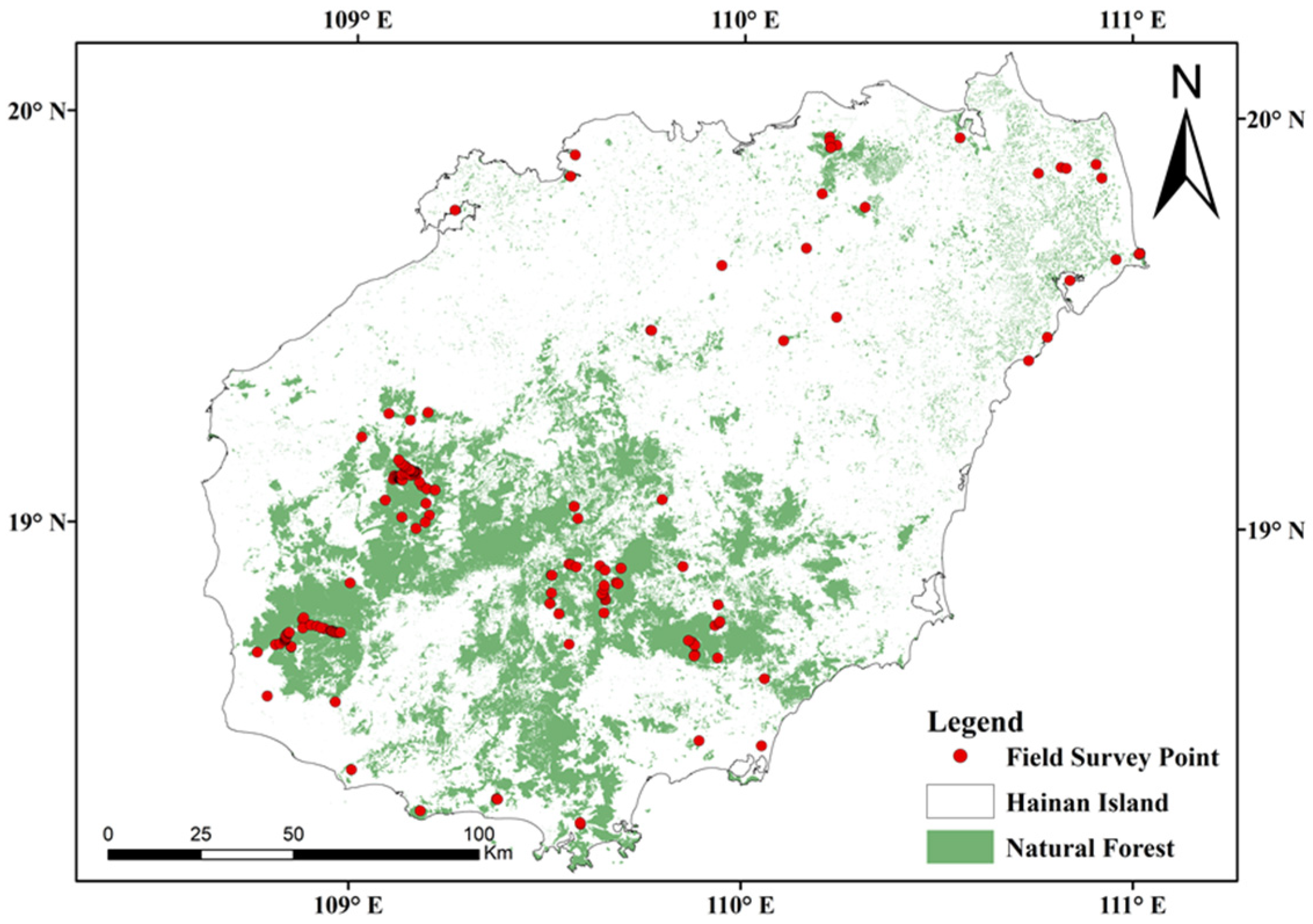
The study carried out field-synchronized data point collection on Hainan Island and obtained a total of 180 sample points for field data. Based on the stratified random sampling method, the sample points were selected to cover a wide range of natural forest types, including typical tropical rainforests, tropical monsoon rainforests, broadleaf evergreen forests, mangrove forests, tropical coniferous forests, and other types of forests. GPS receivers were used in combination with real-time dynamic positioning technology, and measurements were repeated three times for each sample point to reduce random errors, with simultaneous recording of latitude and longitude geographic coordinates and forest tertiary land types. The extent of natural forests on Hainan Island, where the study was carried out, and the distribution of field-synchronized measurements of natural forest sites are shown in Figure 2.

2.3. Methods

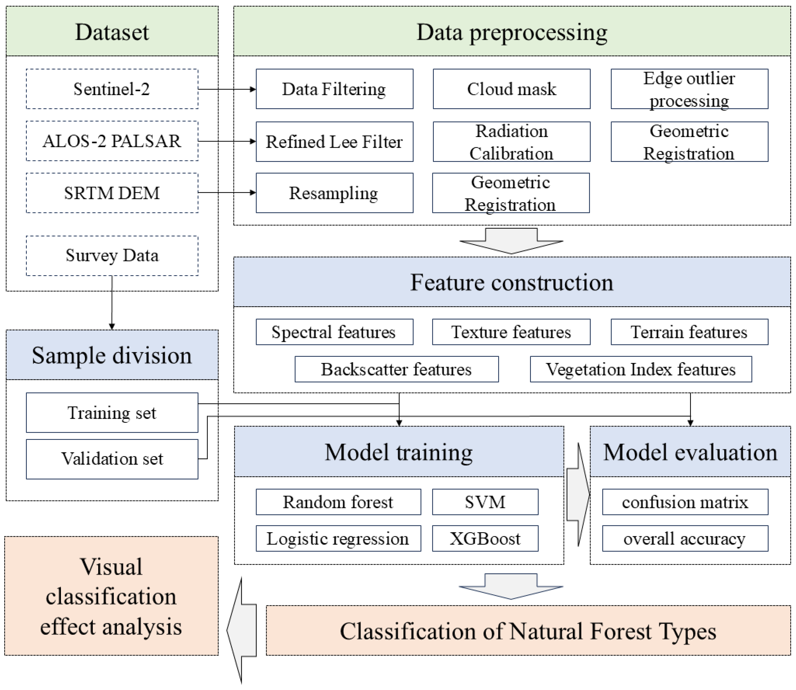
The general technical route of this study is shown in Figure 3. The dataset was constructed based on Sentinel-2, ALOS-2 PALSAR, and SRTM DEM data, and four machine learning models, namely, RF, SVM, LR, and XGBoost, were trained to classify the natural forest types to obtain the results, which were then visualized and analyzed to evaluate the classification performance.

2.3.1. Data Preprocessing

In this study, the Hainan Regional Sentinel-2 Level-2A Surface Reflectance product (COPERNICUS/S2_SR), based on the Google Earth Engine platform, was processed for a full year from May 2022 to April 2023; this already included atmospheric correction processing based on the Sen2Cor algorithm. The joint cloud probability product (COPERNICUS/S2_CLOUD_PROBABILITY) was used for image element-level masking with a 20% cloud probability threshold, and was combined with mask weights to eliminate edge outliers, and a median was synthesized to obtain a de-clouded image. The raw DN values were normalized and converted to surface reflectance and resampled to 10 m resolution. Twelve key bands, including blue light, green light, red light, near-infrared, red edge, and short-wave infrared (B1, B2, B3, B4, B5, B6, B7, B8, B8A, B11, B12), were selected. The ALOS-2 PALSAR data were obtained by DEM-assisted terrain correction and radiometric calibration to obtain the physical quantities of radar scattering cross-section (sigma-naught, σ 0 ), and the noise reduction was performed by using a modified Lee filter (7 × 7 window) to construct a four-channel dataset containing HH, HV polarization, radar vegetation index (RVI), and polarization difference (HH-HV). We selected images with incident angles ranging from 31.41° to 40.56° and fixed the observation azimuth at 90° to minimize the impact of geometric differences on backscattering. The rasterio reproject function was used to map the data to the Sentinel-2 optical image. Bilinear interpolation was used for alignment to ensure that the aligned data were smooth and suitable for subsequent analysis, and multiple data were resampled to a resolution of 10 m. SRTM DEM data were uniformly resampled to a spatial resolution of 10 m, enabling spatial alignment of data from multiple sources.

2.3.2. Feature Construction

Based on ArcGIS combined with field survey coordinates and attribute information, training sample areas of remote sensing images were produced by visual interpretation. According to the attribute characteristics of forest types, vector data of various forest areas were accurately mapped to construct a high-quality sample labeled dataset to ensure the effectiveness of classification model training. Spectral features, vegetation indices, texture features, backscattering features, and terrain features were fused for training the model based on extensive previous forest classification studies, as shown in Table 2.
  • Spectral feature.
    The reflectance values of the visible, near-infrared, and short-wave infrared bands (12 bands) of Sentinel-2 were selected.
  • Vegetation index.
    The vegetation index [37] is an algorithm based on the reflectance spectral information of vegetation canopy for assessing vegetation cover, vigor, growth dynamics, etc. The reflectance of vegetation to different spectra is affected by factors such as plant type and water content. The normalized vegetation index (NDVI) [38], normalized difference water index (NDWI) [39], enhanced vegetation index (EVI) [40], red-edge normalized difference vegetation index (RENDVI) [41], and difference vegetation index (DVI) [42] were calculated in this study.
  • Texture feature.
    Texture is one of the important features for recognizing images, and the Gray-Level Co-occurrence Matrix (GLCM) is a classical method for analyzing statistical texture features [43], which is widely used in image processing and remote sensing analysis for quantitatively portraying the spatial dependence of the pixel gray values of an image. It describes the spatial gray structure of an image by counting the joint probability distribution of pairs of gray values in an image under a particular spatial relationship. Based on the near-infrared band (B8) in the Sentinel-2 image and the HH and HV polarization channels of the ALOS-2 PALSAR image, the three most representative texture features in the GLCM, entropy, contrast, and homogeneity, were selected. A sliding window strategy (7 × 7) was used to traverse the image pixels, and the average values of 0° (horizontal), 45°, 90° (vertical), and 135° were calculated as the final results. Entropy measures the randomness and complexity of the texture, contrast reflects how drastically the gray scale changes, and homogeneity portrays the smoothness or consistency of the image. The computational results in each of the four directions were calculated and then averaged to eliminate the instability caused by the choice of direction, thus enhancing the robustness of the features.
  • Backscattering feature.
    The backscattering coefficient σ0 value (dB) of the dual-polarized (HH and HV) SAR data in the L-band from the ALOS-2 satellite was obtained. The radar vegetation index (RVI) [44] and polarization difference were introduced to characterize the vegetation structural heterogeneity for the tropical vegetation canopy scattering characteristics. An RVI > 0.5 indicates dense vegetation cover, the physical mechanism of which originates from the body scattering-dominated HV polarization enhancement effect.
  • Topographic feature.
    Quantitative topographic factors provide key environmental variables for the delineation of tropical forest types, and the spatial distribution of forest types is closely related to topography. Parameters such as elevation, slope, and slope direction covering Hainan Island were obtained based on the resampled SRTM DEM data.
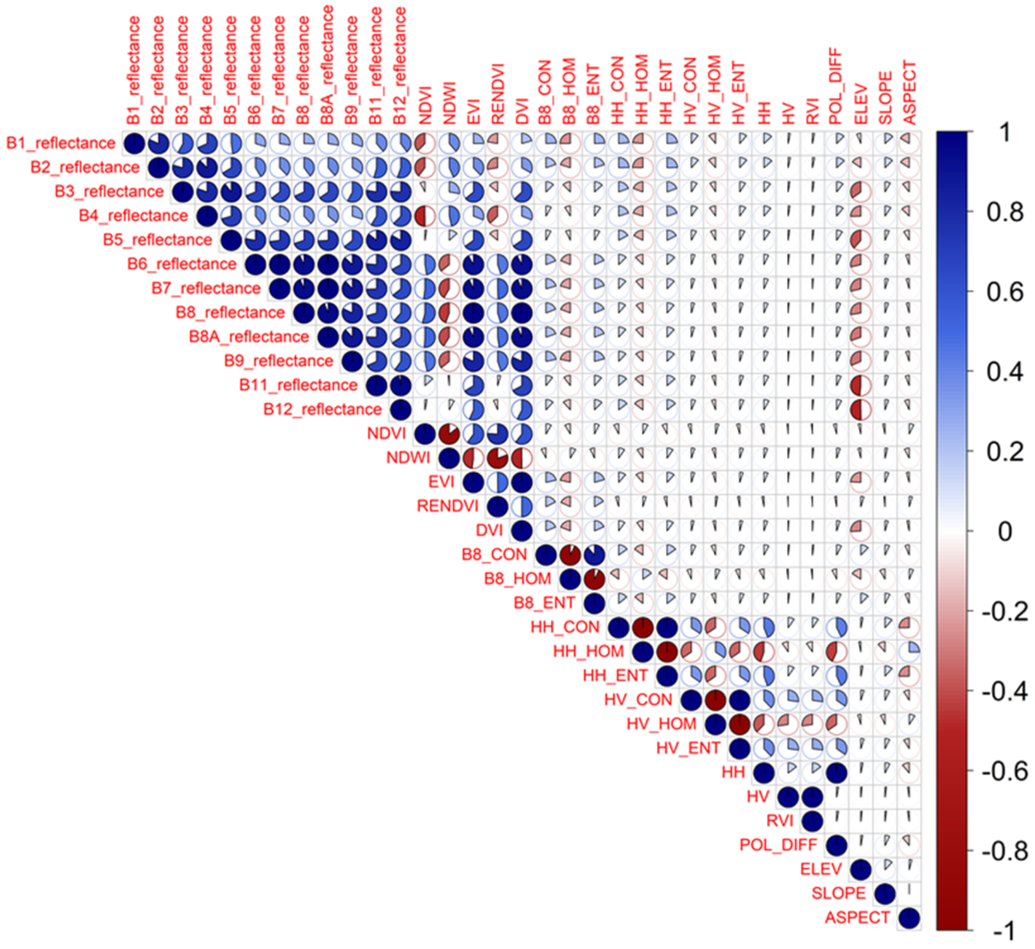
Spearman’s correlation coefficient is a nonparametric statistical method for measuring the monotonic relationship between two variables without assuming that the data follow a normal distribution, and it is suitable for common nonlinear relationships in re-mote sensing data [45]. The coefficient ranges from 1 to 1 , and the closer the value is to ± 1 , the stronger the correlation between the two variables. In order to eliminate the interference of high correlation features on the model performance and to improve the computational speed, this study used Spearman’s Rank Correlation to perform two-by-two correlation analyses on the 33 extracted variable features, and a heat map was drawn based on the correlation matrix (see Figure 4), which is convenient for visualizing the relationships between variable features.
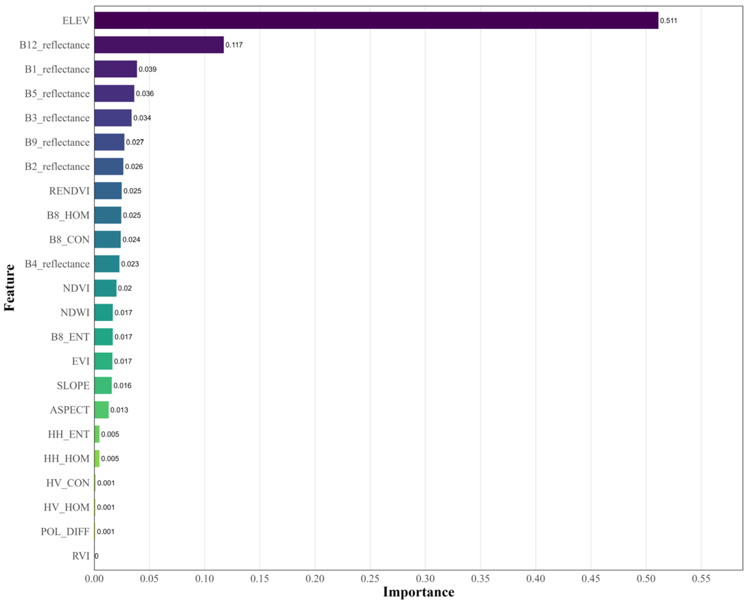
Figure 4. Correlation heat map of the characterized variables. To further improve the generalization ability of the model and reduce the interference of redundant features, we set the threshold of the absolute value of the Spearman correlation coefficient at 0.9, and screened out pairs of highly correlated variables (|r| > 0.9) as redundant feature pairs. The result shows that there are multiple pairs of feature variables with strong correlation. In order to retain the main informative features and avoid information redundancy, this study followed the principle of retaining more informative or representative features, and the variables in the redundant feature pairs were eliminated; 10 variables were deleted. B6_reflectance, B7_reflectance, B8_reflectance, B8A_reflectance, B11_reflectance, DVI, HH_CON, HV_ENT, HH, and HV—a total of 10 variables—were deleted. B1_reflectance, B2_reflectance, B3_reflectance, B4_reflectance, B5_reflectance, B9_reflectance, B12_reflectance, NDVI, NDWI, EVI, RENDVI, B8_HOM, B8_CON, B8_ENT, HH_HOM, HH_ENT, HV_CON, HV_HOM, RVI, POL_DIFF, ELEV, SLOPE, and ASPECT—a total of 23 variables—were left. The feature importance was calculated based on the random forest model, and the selected feature importance ranking graph is shown in Figure 5.
Forests 16 01302 g004
Figure 5. Importance ranking graph of selected features.
Forests 16 01302 g005

2.3.3. Forest Classification System Construction

This study is based on the vegetation classification system proposed by Song et al. in 2011 [46]. In this system, forests belong to one of the vegetation type classes and contain three vegetation type subclasses: coniferous forests, broadleaf forests, and bamboo forests/bamboos. The three vegetation type subclasses, in turn, contain eight vegetation type groups.
However, from the perspective of remote sensing interpretation, there is no study that can realize the classification of 13 species. Most of the existing studies focus on classifying into tropical rainforests, tropical monsoon rainforests, and broadleaf evergreen forests, etc. Therefore, this study mainly tries to categorize the vegetation types mentioned into the vegetation type groups of Hainan natural forests through multi-source remote sensing data, which is called the remote sensing three-level separable type here. Considering the vegetation type groups in Song et al.’s study [46], Shi et al.’s the field survey data [47], the spectral characteristics of the optical remote sensing data, and the backscattering characteristics of the SAR data, the idea of determining the three-level distinguishable types of remote sensing is as follows. There is only one type of evergreen coniferous forest, the tropical coniferous forest, which is identified here as one of the three visible types of remote sensing. Evergreen deciduous forests in Hainan are only scattered evergreen broadleaf forests, and there is no obvious difference between the two, so evergreen broadleaf forests and evergreen deciduous broadleaf mixed forests are combined into one category, and uniformly categorized as evergreen broadleaf forests. Due to their small distribution area, evergreen mossy forests and bamboo forests are not considered as tertiary classifiable types here. Typical tropical rainforests, tropical monsoon rainforests, and mangrove forests can be categorized by spectral features and backscattering features, and can be regarded as three remote sensing classifiable types here.
Through the above analysis, the third level of remote sensing of natural forests in Hainan can be classified into the following five categories by taking advantage of multi-source remote sensing: tropical rainforest, tropical monsoon rainforest, tropical coniferous forest, evergreen broadleaf forest, and mangrove forest. A natural forest remote sensing classification system suitable for Hainan Island was proposed, which can further provide detailed information on the division types of tropical natural forests in Hainan Island; see Table 3.
Tropical rainforests grow in a high-temperature and high-humidity environment and are dominated by tall trees with a complex hierarchical structure and extremely high species richness. Tropical monsoon forests are significantly affected by the monsoon, with obvious seasonal changes; compared with the tropical rainforests, their level is slightly simpler, but they still have rich biological resources. Tropical coniferous forests are mainly distributed in the high-altitude areas of the tropics, dominated by coniferous species. Evergreen broadleaf forests are widely distributed in subtropical and tropical climate zones, dominated by broadleaf evergreen tree species, with a stable ecosystem structure. Mangrove forests are a unique forest type in tropical and subtropical coastal areas, and play an important role in protecting the coastline and preventing wind and waves.

2.3.4. Model Training and Evaluation

In this study, four representative machine learning models were selected for the task of classifying tropical natural forest types, RF, SVM, LR, and XGBoost, respectively, aiming to comprehensively evaluate the adaptability and performance differences of different algorithms in complex tropical natural forest classification tasks.
Among them, RF [48], as a classical integrated learning algorithm, has strong nonlinear modeling capability, can effectively deal with complex relationships between features, is robust to noise and overfitting, and is a widely used baseline model in remote sensing classification research. SVM [49] relies on the RBF kernel function and is suitable for dealing with complex classification problems through nonlinear transformations with highly flexible decision boundaries. LR [50], as a typical linear classifier with good interpretability and high computational efficiency, is suitable as a base model for evaluating the linear separability of sample features. XGBoost [51], as a high-performance boosting algorithm that has emerged in recent years, is capable of automatically modeling the complex interactions and nonlinear relationships among features, and is increasingly widely used in the field of remote sensing classification.
First, the original dataset constructed through field surveys and remote sensing interpretation was divided into a training set (80%) and a validation set (20%) using stratified random sampling to ensure data distribution consistency and avoid sampling bias. Subsequently, model construction and training analysis were conducted for the four representative classification algorithms selected. The sample sizes for each classification category are shown in Table 4.
The number of decision trees (n_estimstors) of the XGBoost model is 500, the maximum depth of a single tree is 10, and the learning rate is 0.24. The model scored 0.89 on the validation set, which has strong generalization ability. The learning curve of the XGBoost model is shown in Figure 6, showing that the loss of the training set and the validation set gradually decrease and stabilize with the increase in the number of training rounds, and there is no obvious overfitting, which further verifies the convergence of the model. The SVM model kernel is the RBF kernel, the gamma is 0.1, and the regularization parameter C is 100. The number of decision trees (n_estimators) of the RF model is 100, the max_depth is 12, the minimum number of samples required for node splitting is 10, the minimum number of samples for leaf nodes is 5, and the random seed is 42. The LR model uses a logarithmic loss function, with a maximum number of iterations of 200, a random_state of 42, and a convergence tolerance of 1 × 10     5 . These parameters can ensure the repeatability of the experiment and improve the classification accuracy.
In this study, the performance of the model was evaluated using several categorical metrics. The confusion matrix [52] enables visualization of the model’s prediction performance on each category. The precision rate, recall rate, and F1 score were also calculated to analyze the model performance in more detail. The precision rate reflects the accuracy of the model in positive category prediction, while the recall rate evaluates the model’s ability in detecting all positive category samples. The F1 score, as a composite of precision and recall, provides a more comprehensive view of model performance. In addition, the use of five-fold cross-validation (k = 5) to assess the stability and generalization ability of the model ensured consistent performance of the model on different data subsets, which further enhanced the robustness and reliability of the evaluation results. Accuracy, as an overall performance metric, demonstrates the predictive accuracy of the model on all samples. These categorical metrics enable a comprehensive assessment of the model’s strengths and weaknesses, thus providing guidance for subsequent optimization and improvement.

3. Results and Discussion

3.1. Results

3.1.1. Classification Results

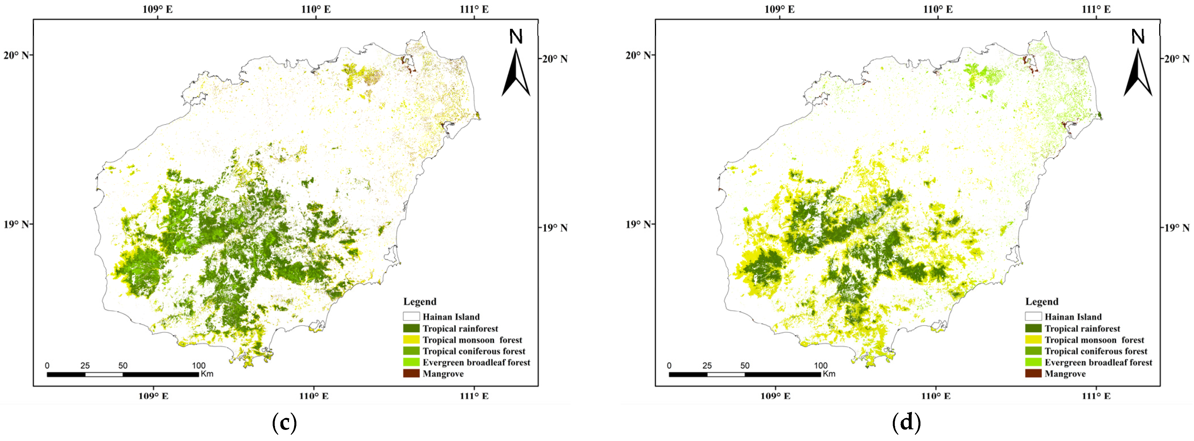
For tropical natural forest classification, we used the trained RF, SVM, LR, and XGBoost models to predict the five types within the natural forest range, and the classification results are shown in Figure 7.
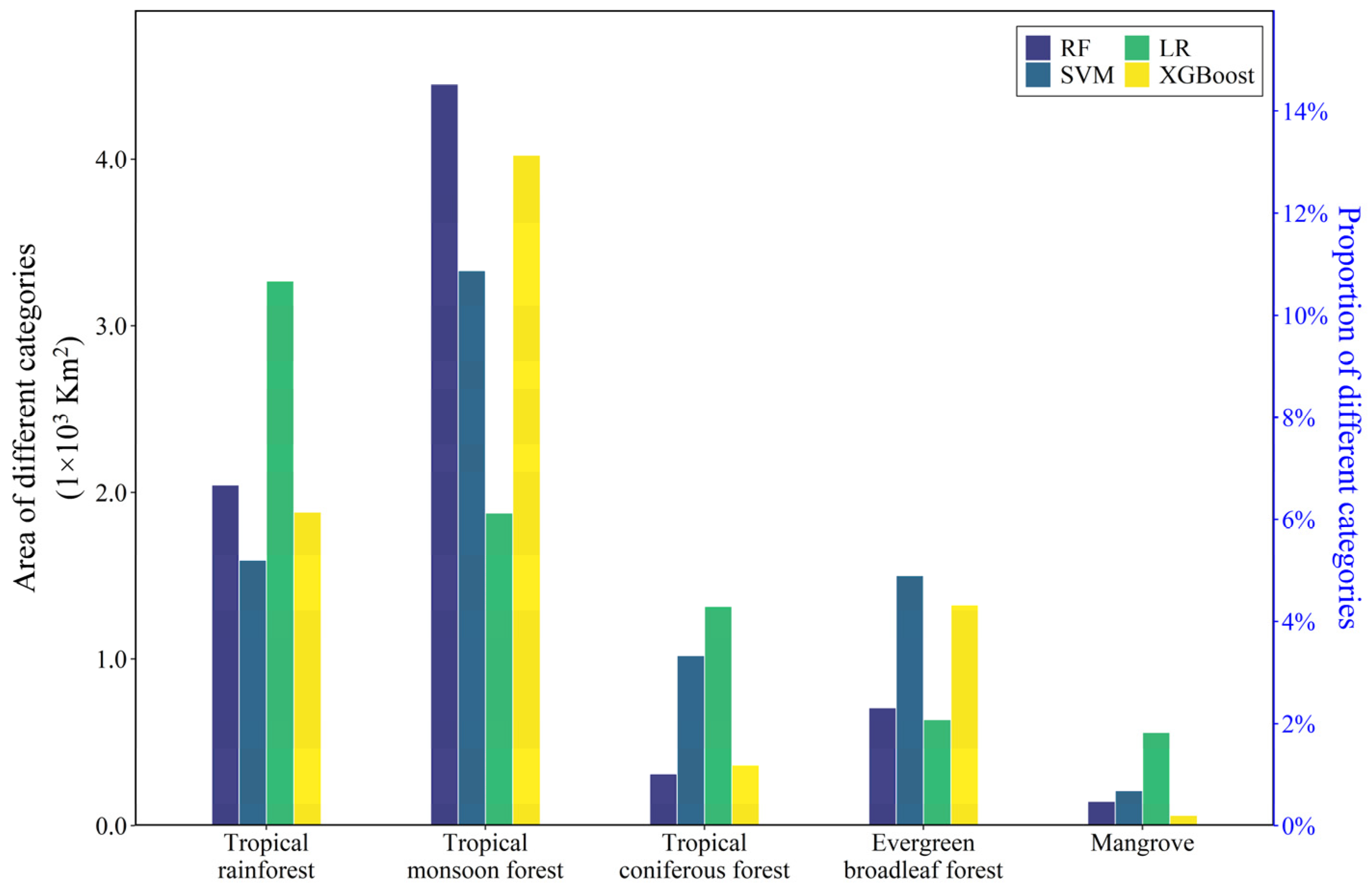
Among them, none of the three models, RF, SVM, and XGBoost, showed extensive misclassification, and mangrove forests were most accurately detected in the natural forest range. The classification results showed that tropical rainforests and tropical monsoon forests occupied a larger area, indicating their importance in terms of biodiversity and ecosystem complexity. Tropical coniferous forests occupied a relatively small area, suggesting that their distribution is more restricted and may be dependent on specific climatic or soil conditions. Evergreen broadleaf forests, which are adapted to warm and humid environments, and mangrove forests, which cover mainly plains and coastal areas, perform important ecological functions in coastal areas, such as preventing coastal erosion and providing habitat.
Figure 8 shows a comparison of the area (left axis) and proportion (right axis) of five different tropical natural forest types, tropical rainforest (TR), tropical monsoon forest (TMF), tropical coniferous forest (TCF), evergreen broadleaf forest (EBF), and mangrove forest (Man) under different machine learning algorithms (RF, SVM, LR, and XGBoost).
There were some differences in the percentage of classification results of the four models for TR, among which the LR model had the highest percentage, indicating that it believed that this type of forest occupies a larger ecological proportion. The SVM results have the lowest percentage, showing that the model may be more conservative in the identification of tropical rainforests, and the percentages of the results of RF and XGBoost are in between, with a relatively stable performance, accounting for an average of one-fourth. For the classification results of TMF, the prediction proportions of RF and XGBoost were very close to each other, and both considered TMF as one of the forest types with the highest area proportion; the SVM model had the second highest proportion, which is somewhat different from the results of RF and XGBoost, but still within a reasonable range, and the results of LR have the lowest proportion, which is in sharp contrast with the results of other models. The LR model was significantly higher than the other models in the percentage of TCF, indicating that it is more sensitive to the identification of tropical coniferous forests, and may classify part of the edge area as this type. SVM is second, and the results of RF and XGBoost are close, with a relatively low percentage, and the performance was more consistent. Regarding EBF classification, the SVM and XGBoost models had a higher percentage of predictions. The Man classification results of each model accounted for the smallest area.

3.1.2. Accuracy of Classification Results

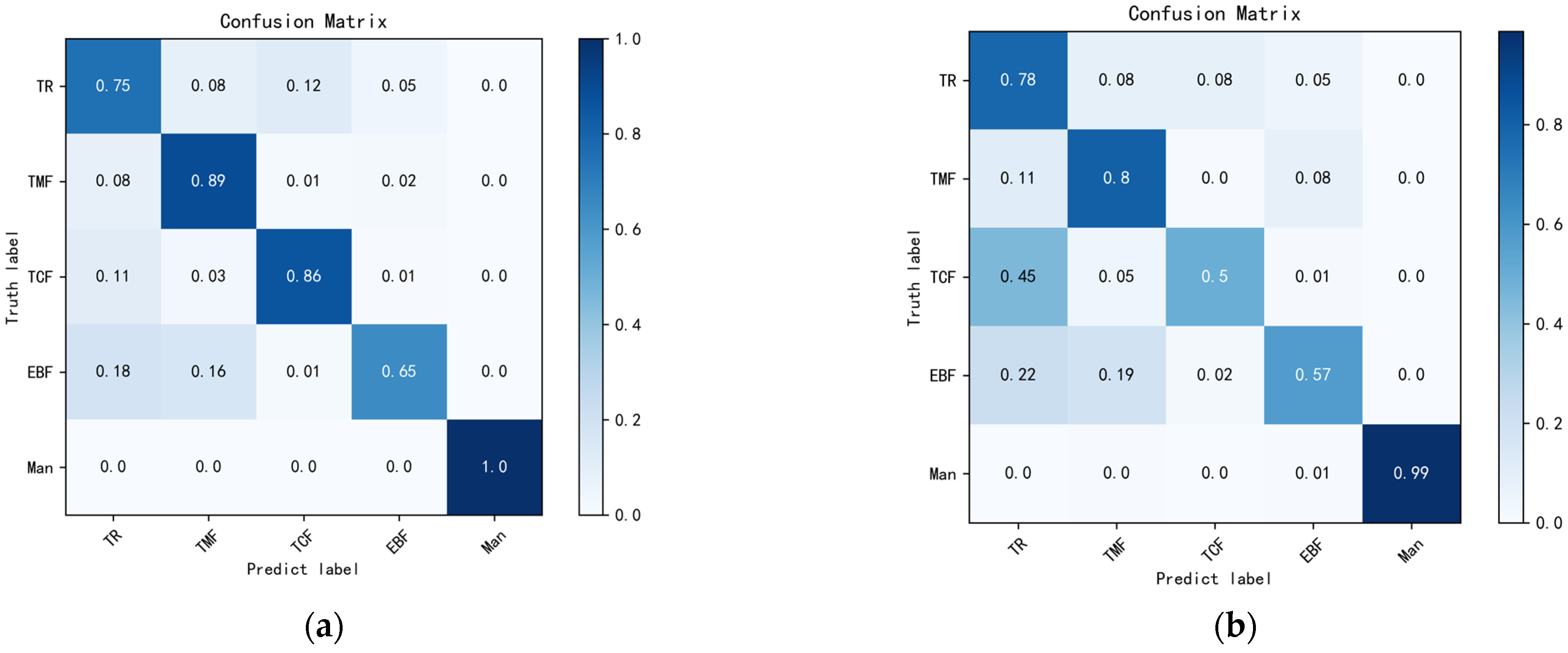
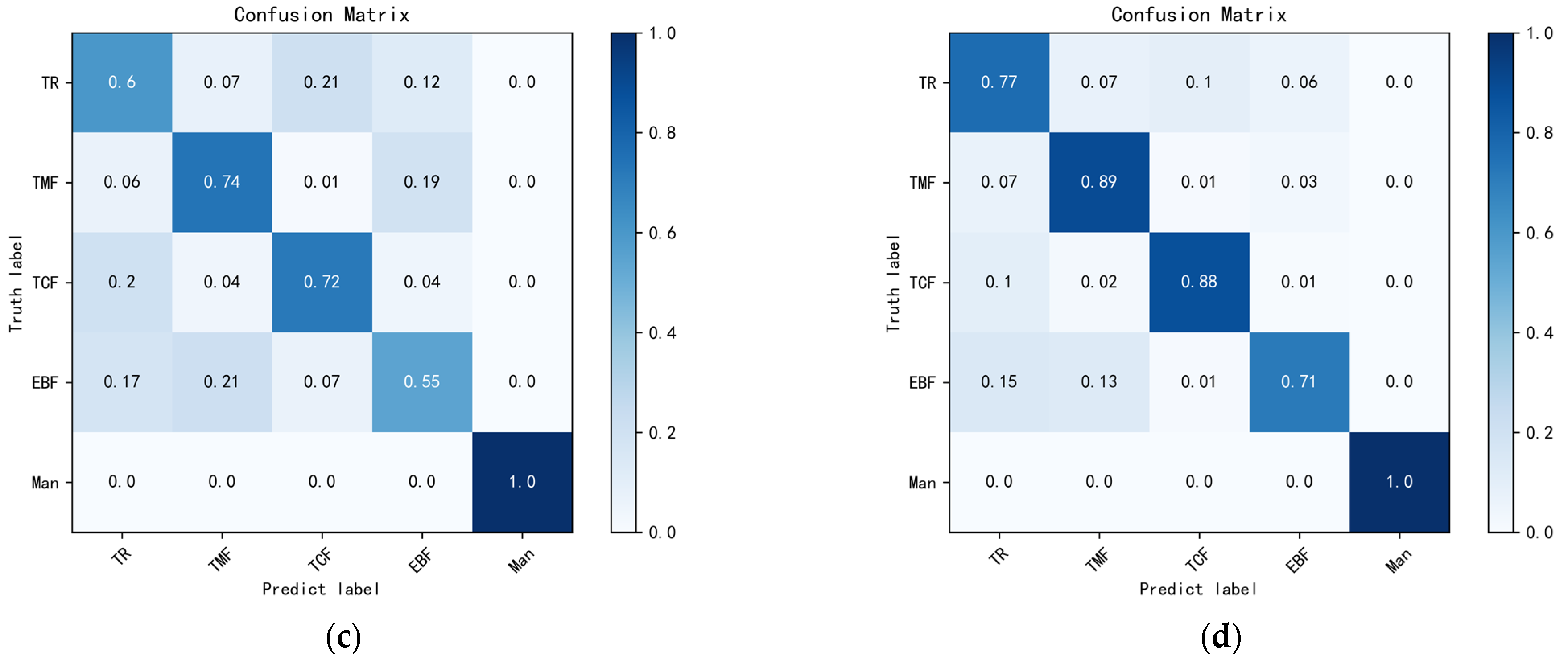
Based on the validation set, the results of the confusion matrix calculation for the four machine learning models in the natural forest classification task are shown in Figure 9. The comparison revealed that the XGBoost model performed the best, achieving the highest classification accuracy on most forest types, followed in order by RF, SVM, and LR. Specifically, XGBoost achieved classification accuracies of 0.77 (TR), 0.89 (TMF), 0.88 (TCF), 0.71 (EBF), and 1.0 (Man) for the five types of forests, which fully reflected its strong modeling ability for complex nonlinear features. RF, on the other hand, showed good robustness and equalization, and especially good results in classifying TMF (0.89) and Man (1.0), but there was still a small amount of confusion regarding EBF. In contrast, SVM was more effective in recognizing TR (0.78) and Man (1.00), but there was an obvious deficiency in recognizing EBF, indicating that EBF has high feature similarity with other forest types, which made it difficult for SVM to accurately classify it. The LR model had the worst classification effect, mainly due to the limitation of its linear modeling ability, which made it difficult to capture the complex spectral and structural features of natural forests. It is worth notice that the classification effect of mangrove was excellent in all four models, indicating that the mangrove is more different from other categories and is easy to distinguish.
Comparing and analyzing the experimental data, the overall accuracy is shown in Table 5.
XGBoost shows significant advantages in the complex tropical natural forest classification task. Its overall accuracy (0.89), F1 score (0.88), and Kappa coefficient (0.82) are significantly higher than other models, verifying the effectiveness of gradient boosting in complex tropical natural forest classification. The results for RF are also more robust, with an overall accuracy of 0.83 and a Kappa coefficient of 0.77. SVM has the third-best results, with an overall accuracy of only 0.73. LR, as a representative of the linear model, significantly lags behind in all metrics, with an overall accuracy of 0.68 and a Kappa coefficient of 0.56 (Table 5).
As can be seen from Table 6, the classification performance of tropical rainforests is low, especially in SVM and LR models, with the lowest user accuracy of 0.5 in SVM, which may be related to the high density of vegetation cover in tropical rainforests, resulting in spectral characteristics similar to other dense forest types. The producer accuracy and F1 score of tropical coniferous forests in the SVM model are significantly lower than those of other models. This may be because there are fewer tropical coniferous forests and less sample data, resulting in insufficient model training. In contrast, mangroves show extremely high classification accuracy due to their unique spectral characteristics. The categories with low precision and recall are mainly concentrated in tropical rainforests, tropical coniferous forests, and evergreen broadleaf forests. The systematic errors of this classification are mainly concentrated in the similarity of vegetation structure and the limitation of remote sensing image resolution.

3.1.3. Feature Analysis

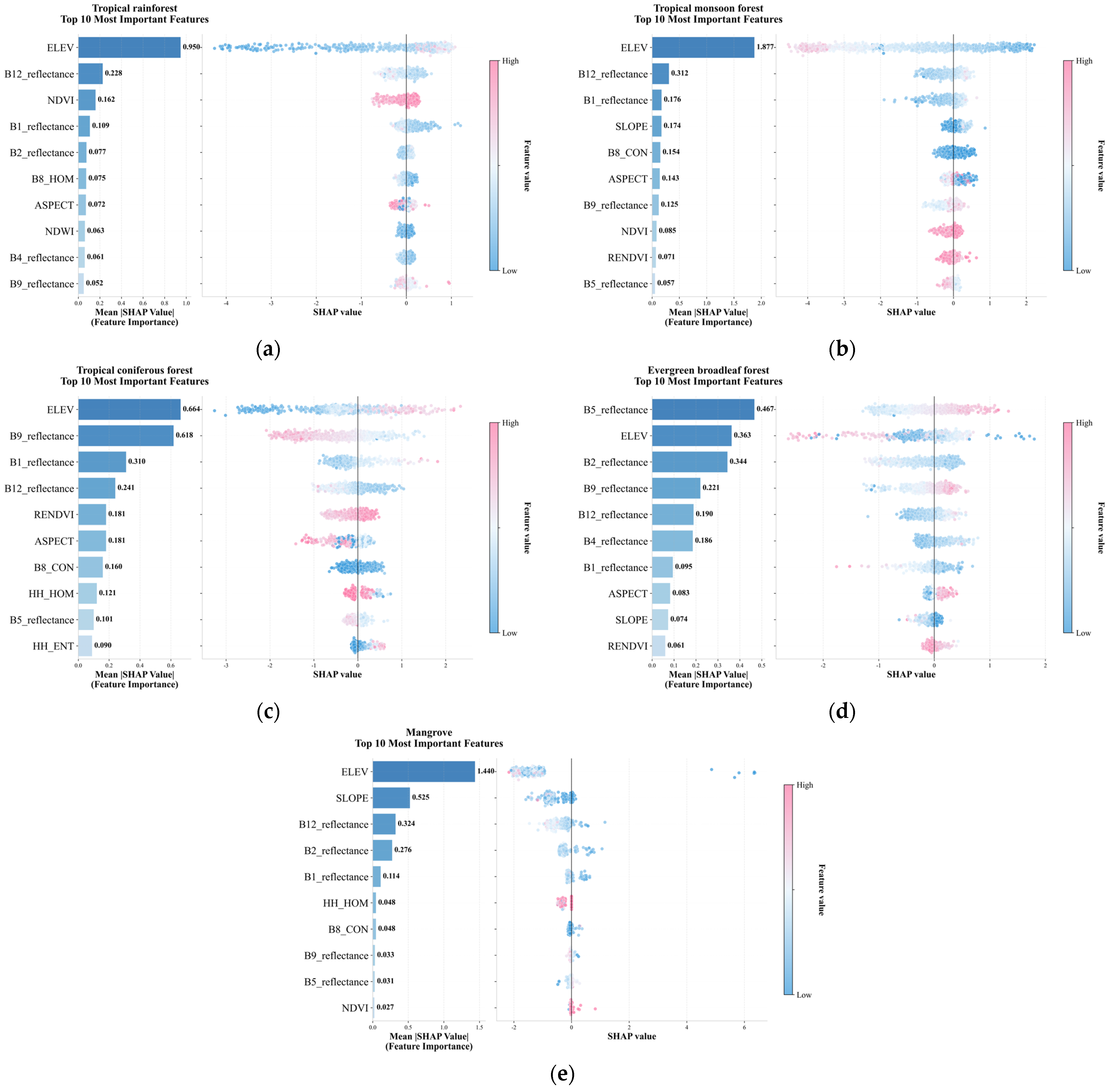
Shapley Additive exPlanations (SHAP), proposed by Lundberg et al. [53], was used to interpret the output of the model. The SHAP values provided an estimation of the contribution of each feature to the model based on game theory and local interpretation. The feature importance ranking and SHAP values based on the optimal model XGBoost are shown in Figure 10. It was found that topographic features had the highest importance inside the multi-category forest classification, and these results are reasonable. Because forest growth is more likely to be influenced by hydrothermal conditions, the elevation of the terrain affects the hydrothermal conditions of the environment.
Figure 10 demonstrates the ordering of the top ten important features in the classification of the five forest types, which are represented by five subplots corresponding to the classification categories in (a), (b), (c), (d), and (e), respectively. It can be found that elevation is the most important feature for the identification and classification of tropical rainforests, tropical monsoon rainforests, tropical coniferous forests, and mangrove forests, indicating its wide applicability. The red-edge band (B5) showed significant feature importance in identifying broadleaf evergreen forests, and the short-wave infrared band (B12) showed high importance in the classification of tropical rainforests and tropical monsoon rainforests. Vegetation indices such as NDVI and RENDVI contributed to the classification of tropical rainforests and tropical coniferous forests, respectively.
These results are reasonable. Topographic features were found to be of the highest importance within the multi-category forest classification, where forest growth is mainly influenced by hydrothermal conditions, and then the elevation of the terrain affects the spatial distribution of forest types by influencing the hydrothermal conditions of the environment. Meanwhile, spectral characteristics are also an important basis for recognizing different forest types, because different vegetation classes have different physical structures and biochemical parameters, and spectral reflectance may also vary.
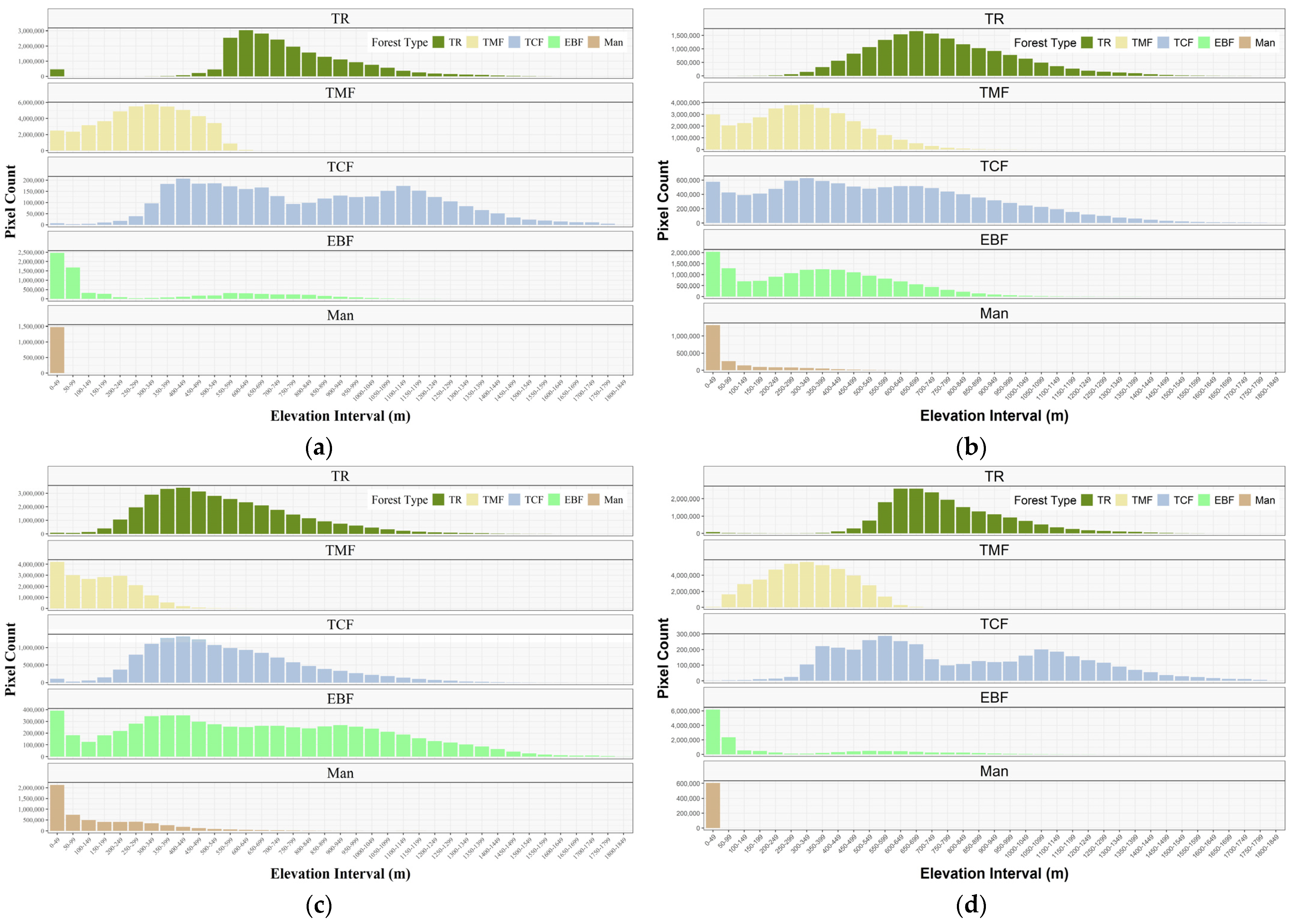
Figure 11 illustrates the distribution of pixels in different elevation intervals for tropical natural forest types predicted by the four classification models. It can be found that all four models predicted that tropical rainforests are mainly concentrated in low- to medium-altitude regions, and tropical monsoon forests are distributed in low-altitude regions. The RF, SVM, and XGBoost models predicted a wider distribution of tropical coniferous forests, concentrating in middle- to high-altitude regions, while the LR model appeared to predict their concentration in low-altitude regions. Evergreen broadleaf forests are concentrated in low-elevation regions in RF and XGBoost model predictions, and SVM and LR have an extension of their distribution range in middle-elevation regions. Mangrove forests are concentrated in the lowest elevation region (0–49 m) in all four models.

3.2. Discussion

3.2.1. Analysis of the Strengths of Joint Optical and SAR in the Local Area

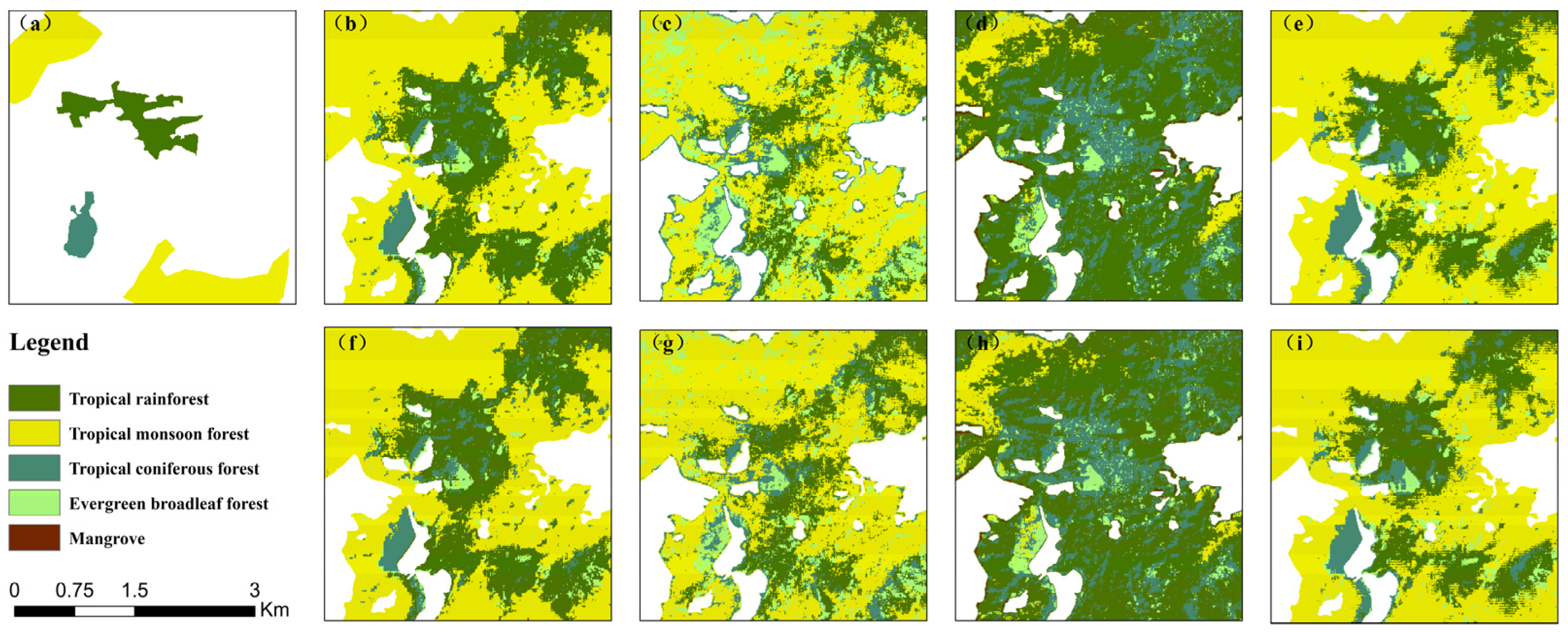
In this subsection, two regions were selected to carry out the analysis of the results of the joint classification of optical and SAR data in comparison with the optical classification alone in more detail. The results for region 1 are shown in Figure 12.
The label truth values provided criteria for the comparison of results from (a) in Figure 10. RF, SVM, and XGBoost improved in joint classification results compared to their optical classifications. RF performed optical classification in joint classification recognition of tropical rainforests in terms of boundary clarity and detailing of small plots. XGBoost had the best results in joint classification; not only did it have the highest accuracy in boundary recognition of all forest types, but it also reduced misclassification of tropical monsoon rainforests and tropical coniferous forests, while its optical classification was slightly inferior in boundary processing. And the results of the LR model joint classification in tropical rainforest identification were better than those of optical classification.
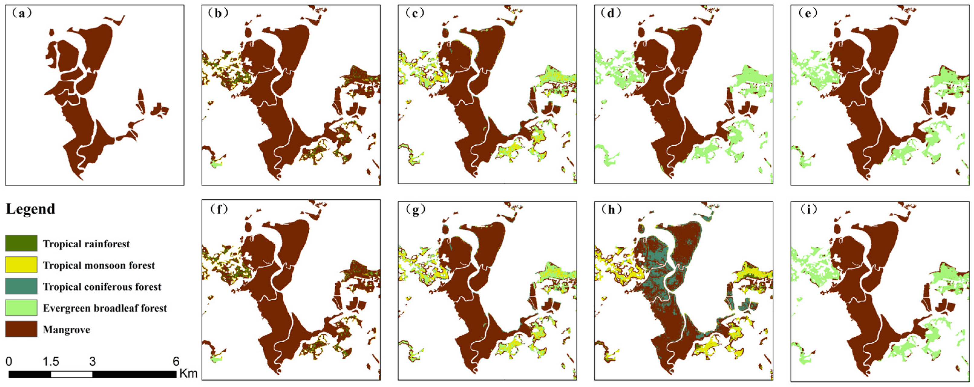
The results of region 2 are shown in Figure 13. The classification results of region 2 showed that the classification accuracy of the combined optical and SAR data was significantly better than that of the optical data alone. Among the LR model optical classification results, there is an obvious misclassification phenomenon, and the recognition accuracy of the joint data classification for mangrove forests was significantly improved.

3.2.2. Implications of the Present Study and the Future Work

Following our research objectives, the findings of this paper would be useful in three aspects. First, this study constructed a classification system applicable to tropical natural forests by utilizing field survey data and comprehensively investigating the classification systems of previous studies, such as vegetation ecology. This system can effectively distinguish different forest types, including tropical rainforest, tropical monsoon rainforest, tropical coniferous forest, evergreen broadleaf forest, and mangrove forest, which provides a scientific basis for the fine analysis of tropical natural forests. Second, this study made full use of the advantages of optical remote sensing data and SAR data to complement each other, which significantly improved the classification accuracy, with a classification accuracy of 0.89, an F1 score of 0.88, and a Kappa coefficient of 0.82. Third, by comparing four classical machine learning algorithms, namely, RF, SVM, LR, and XGBoost, the best joint classification based on XGBoost was constructed to realize the fine classification of tropical natural forests in the study area of Hainan Island, which provides a reference for similar forest resource monitoring.
However, the present study also has some limitations. This study mainly used four classical machine learning models instead of deep learning models, which is because this study is aimed at the classification of tropical natural forests, and the constructed sample set comes from measured data and the research dataset of Zhang et al. [54]. These data are in the point scale form. While deep learning semantic segmentation algorithms require high-precision images to be manually sketched to generate training samples, the current publicly available data sources are not sufficient to support the classification between tropical natural forests. This situation limits the application of deep learning semantic segmentation algorithms. Chaity et al. [55] studied tree species recognition technology based on convolutional neural networks in complex forest scenes and analyzed the impact of different spatial, spectral, and scale resolutions on classification accuracy. The results showed that under complex conditions, the accuracy of the SVM model results and the lightweight CNN model at a spatial resolution of 30 m were basically equivalent, both around 55%. Lai et al. [56] analyzed various factors that affect forest classification, such as classification algorithm and sample size, among which the RF algorithm had the best classification results, with an overall accuracy of 87%. Chen et al. [57] used a deep learning network to classify subtropical natural forests based on the fusion of high-resolution drone imagery and multispectral imagery, with an overall accuracy of about 81%.
Our future work will focus on the development and application of more novel algorithmic models. On the one hand, we will try to apply deep learning techniques such as convolutional neural networks to combine high-resolution images to further improve the classification accuracy. On the other hand, it is also recommended to develop new individual or hybrid models to combine the advantages of different models, and further improve the classification accuracy and applicability of the classification models based on the fusion of multi-source remote sensing data, to provide technical support for the protection of tropical natural forests.

4. Conclusions

Hainan Island in China is rich in tropical forest resources, and the in-depth study of tropical natural forests requires accurate and fine classification. In this study, the performance of four machine learning models, namely RF, SVM, LR, and XGBoost, was comprehensively evaluated for the classification of tropical natural forests by jointly utilizing the multispectral data of Sentinel-2 and ALOS-2 PALSAR data. The results show that XGBoost performed best in most forest types, especially in modeling complex nonlinear features with significant advantages, and the accuracy of all metrics was better than that of other models. RF showed good robustness and balance in classifying tropical monsoon rainforests and mangrove forests, but there was still some confusion among broadleaf evergreen forest classes. SVM performed well in the identification of tropical rainforests, tropical monsoon rainforests, and mangrove forests, but had difficulties in the classification of tropical coniferous forests and broadleaf evergreen forests. The LR model had the worst accuracy due to the limitations of its linear modeling.
We also identified topographic features (e.g., elevation) as key features in the classification of tropical rainforests, tropical monsoon rainforests, tropical coniferous forests, and mangrove forests, suggesting that topography influences the spatial distribution of forest types by affecting the hydrothermal conditions and thus the spatial distribution of forest types. The distribution of pixels at different elevation intervals of the classification results further indicated the distribution pattern of natural forest types. Combining the results of the four models resulted in predictions that tropical rainforests were concentrated in the low- to middle-elevation regions, tropical monsoon forests in the low-elevation regions, and tropical coniferous forests in the middle- to high-elevation regions, whereas broadleaf evergreen forests were concentrated in the low-elevation regions, and mangrove forests were distributed in the lowest elevation regions.
The classification results of combining optical and SAR data were compared to the classification of optical data alone, and it was found that the joint classification accuracy of all four models is improved, and the boundary identification is made more accurate, by comparing region 1 and region 2. Comprehensively comparing the performance of the four methods, XGBoost has the best results in overall accuracy (0.89), F1 score (0.88), and Kappa coefficient (0.82); RF is second and more robust; SVM has some advantages in some types; and LR has the worst results in all the metrics due to the limitation of its linear modeling capability. In the next step, we will enrich the data sources, for example, by using hyperspectral data, and adopt deep learning algorithms to further improve the classification accuracy. Future research should investigate the applicability of these classification frameworks in other tropical regions, integrate seasonal dynamics, and explore the use of time-series data to enhance temporal generalization.

Author Contributions

Conceptualization, X.L. and W.F.; methodology, Q.X.; validation, Q.X. and C.H.; investigation, W.F. and J.S.; writing—original draft preparation, Q.X.; writing—review and editing, Q.X. and S.X.; project administration, W.Y. and X.L.; funding acquisition, X.L. and H.L. All authors have read and agreed to the published version of the manuscript.

Funding

This research was funded by the Science and Technology special fund of Hainan Province, China, grant number ZDYF2023SHFZ129, the Guangxi Major Science and Technology Project, grant number (GuikeAA24206025), the Hainan Provincial Natural Science Foundation of China, grant number 424CXTD433, and the Hainan Provincial ‘Nanhaixinxing’ Foundation of China, grant number NHXXRCXM202352.

Data Availability Statement

The dataset and codes used in this study are available from the corresponding authors upon request.

Conflicts of Interest

The authors declare no conflicts of interest.

References

  1. Lewis, S.L.; Wheeler, C.E.; Mitchard, E.T.A.; Koch, A. Restoring Natural Forests Is the Best Way to Remove Atmospheric Carbon. Nature 2019, 568, 25–28. [Google Scholar] [CrossRef]
  2. FAO. Global Forest Resources Assessment 2020; FAO: Roma, Italy, 2020; ISBN 978-92-5-132581-0. [Google Scholar]
  3. Marden, M.; Lambie, S.; Phillips, C. Biomass and Root Attributes of Eight of New Zealand’s Most Common Indigenous Evergreen Conifer and Broadleaved Forest Species during the First 5 Years of Establishment. N. Z. J. For. Sci. 2018, 48, 9. [Google Scholar] [CrossRef]
  4. Qin, Y.; Wang, D.; Ziegler, A.D.; Fu, B.; Zeng, Z. Impact of Amazonian Deforestation on Precipitation Reverses between Seasons. Nature 2025, 639, 102–108. [Google Scholar] [CrossRef] [PubMed]
  5. Santos, E.G.; Svátek, M.; Nunes, M.H.; Aalto, J.; Senior, R.A.; Matula, R.; Plichta, R.; Maeda, E.E. Structural Changes Caused by Selective Logging Undermine the Thermal Buffering Capacity of Tropical Forests. Agric. For. Meteorol. 2024, 348, 109912. [Google Scholar] [CrossRef]
  6. Harris, N.L.; Gibbs, D.A.; Baccini, A.; Birdsey, R.A.; de Bruin, S.; Farina, M.; Fatoyinbo, L.; Hansen, M.C.; Herold, M.; Houghton, R.A.; et al. Global Maps of Twenty-First Century Forest Carbon Fluxes. Nat. Clim. Chang. 2021, 11, 234–240. [Google Scholar] [CrossRef]
  7. Mitchard, E.T.A. The Tropical Forest Carbon Cycle and Climate Change. Nature 2018, 559, 527–534. [Google Scholar] [CrossRef]
  8. Baccini, A.; Goetz, S.J.; Walker, W.S.; Laporte, N.T.; Sun, M.; Sulla-Menashe, D.; Hackler, J.; Beck, P.S.A.; Dubayah, R.; Friedl, M.A.; et al. Estimated Carbon Dioxide Emissions from Tropical Deforestation Improved by Carbon-Density Maps. Nat. Clim. Chang. 2012, 2, 182–185. [Google Scholar] [CrossRef]
  9. Gatti, L.V.; Basso, L.S.; Miller, J.B.; Gloor, M.; Gatti Domingues, L.; Cassol, H.L.G.; Tejada, G.; Aragão, L.E.O.C.; Nobre, C.; Peters, W.; et al. Amazonia as a Carbon Source Linked to Deforestation and Climate Change. Nature 2021, 595, 388–393. [Google Scholar] [CrossRef] [PubMed]
  10. Chen, Y.; Yang, Q.; Mo, Y.; Yang, X.; Li, D.; Hong, X. A study on the niches of the state’s key protected plants in Bawangling, Hainan Island. Chin. J. Plant Ecol. 2014, 38, 576–584. [Google Scholar]
  11. Gibson, L.; Lee, T.M.; Koh, L.P.; Brook, B.W.; Gardner, T.A.; Barlow, J.; Peres, C.A.; Bradshaw, C.J.A.; Laurance, W.F.; Lovejoy, T.E.; et al. Primary Forests Are Irreplaceable for Sustaining Tropical Biodiversity. Nature 2011, 478, 378–381. [Google Scholar] [CrossRef] [PubMed]
  12. Flores, B.M.; Montoya, E.; Sakschewski, B.; Nascimento, N.; Staal, A.; Betts, R.A.; Levis, C.; Lapola, D.M.; Esquível-Muelbert, A.; Jakovac, C.; et al. Critical Transitions in the Amazon Forest System. Nature 2024, 626, 555–564. [Google Scholar] [CrossRef]
  13. Yu, T.; Wu, W.; Gong, C.; Li, X. Residual Multi-Attention Classification Network for A Forest Dominated Tropical Landscape Using High-Resolution Remote Sensing Imagery. ISPRS Int. J. Geo-Inf. 2021, 10, 22. [Google Scholar] [CrossRef]
  14. Reiche, J.; Lucas, R.; Mitchell, A.L.; Verbesselt, J.; Hoekman, D.H.; Haarpaintner, J.; Kellndorfer, J.M.; Rosenqvist, A.; Lehmann, E.A.; Woodcock, C.E.; et al. Combining Satellite Data for Better Tropical Forest Monitoring. Nat. Clim Chang. 2016, 6, 120–122. [Google Scholar] [CrossRef]
  15. Moreira, A.; Prats-Iraola, P.; Younis, M.; Krieger, G.; Hajnsek, I.; Papathanassiou, K.P. A Tutorial on Synthetic Aperture Radar. IEEE Geosci. Remote Sens. Mag. 2013, 1, 6–43. [Google Scholar] [CrossRef]
  16. Kulkarni, S.C.; Rege, P.P. Pixel level fusion techniques for SAR and optical images: A review. Inf. Fusion 2020, 59, 13–29. [Google Scholar] [CrossRef]
  17. Heckel, K.; Urban, M.; Schratz, P.; Mahecha, M.D.; Schmullius, C. Predicting Forest Cover in Distinct Ecosystems: The Potential of Multi-Source Sentinel-1 and -2 Data Fusion. Remote Sens. 2020, 12, 302. [Google Scholar] [CrossRef]
  18. Dobrinić, D.; Gašparović, M.; Medak, D. Sentinel-1 and 2 Time-Series for Vegetation Mapping Using Random Forest Classification: A Case Study of Northern Croatia. Remote Sens. 2021, 13, 2321. [Google Scholar] [CrossRef]
  19. Zhang, Z.; Moore, J.C. Remote Sens.; Elsevier: Amsterdam, The Netherlands, 2015; pp. 111–124. ISBN 978-0-12-800066-3. [Google Scholar]
  20. Ouchi, K. Recent Trend and Advance of Synthetic Aperture Radar with Selected Topics. Remote Sens. 2013, 5, 716–807. [Google Scholar] [CrossRef]
  21. Balling, J.; Slagter, B.; van der Woude, S.; Herold, M.; Reiche, J. ALOS-2 PALSAR-2 ScanSAR and Sentinel-1 Data for Timely Tropical Forest Disturbance Mapping: A Case Study for Sumatra, Indonesia. Int. J. Appl. Earth Obs. Geoinf. 2024, 132, 103994. [Google Scholar] [CrossRef]
  22. Joshi, N.; Baumann, M.; Ehammer, A.; Fensholt, R.; Grogan, K.; Hostert, P.; Jepsen, M.R.; Kuemmerle, T.; Meyfroidt, P.; Mitchard, E.T.A.; et al. A Review of the Application of Optical and Radar Remote Sensing Data Fusion to Land Use Mapping and Monitoring. Remote Sens. 2016, 8, 70. [Google Scholar] [CrossRef]
  23. Balling, J.; Verbesselt, J.; De Sy, V.; Herold, M.; Reiche, J. Exploring Archetypes of Tropical Fire-Related Forest Disturbances Based on Dense Optical and Radar Satellite Data and Active Fire Alerts. Forests 2021, 12, 456. [Google Scholar] [CrossRef]
  24. Fan, Y.; Qian, Y.; Gong, W.; Chu, Z.; Qin, Y.; Muhetaer, P. Multi-Level Interactive Fusion Network Based on Adversarial Learning for Fusion Classification of Hyperspectral and LiDAR Data. Expert Syst. Appl. 2024, 257, 125132. [Google Scholar] [CrossRef]
  25. Zhu, Q.; Guo, H.; Zhang, L.; Liang, D.; Liu, X.; Wan, X.; Liu, J. Tropical Forests Classification Based on Weighted Separation Index from Multi-Temporal Sentinel-2 Images in Hainan Island. Sustainability 2021, 13, 13348. [Google Scholar] [CrossRef]
  26. Persson, M.; Lindberg, E.; Reese, H. Tree Species Classification with Multi-Temporal Sentinel-2 Data. Remote Sens. 2018, 10, 1794. [Google Scholar] [CrossRef]
  27. Ye, N. Indigenous Forest Classification in New Zealand—A Comparison of Classifiers and Sensors. Int. J. Appl. Earth Obs. Geoinf. 2021, 102, 102395. [Google Scholar] [CrossRef]
  28. Martins, G.B.; La Rosa, L.E.C.; Happ, P.N.; Coelho, L.C.T.; Santos, C.J.F.; Feitosa, R.Q.; Ferreira, M.P. Deep Learning-Based Tree Species Mapping in a Highly Diverse Tropical Urban Setting. Urban For. Urban Green. 2021, 64, 127241. [Google Scholar] [CrossRef]
  29. Lobo Torres, D.; Queiroz Feitosa, R.; Nigri Happ, P.; Elena Cué La Rosa, L.; Marcato Junior, J.; Martins, J.; Olã Bressan, P.; Gonçalves, W.N.; Liesenberg, V. Applying Fully Convolutional Architectures for Semantic Segmentation of a Single Tree Species in Urban Environment on High Resolution UAV Optical Imagery. Sensors 2020, 20, 563. [Google Scholar] [CrossRef]
  30. Qin, H.; Zhou, W.; Yao, Y.; Wang, W. Individual Tree Segmentation and Tree Species Classification in Subtropical Broadleaf Forests Using UAV-Based LiDAR, Hyperspectral, and Ultrahigh-Resolution RGB Data. Remote Sens. Environ. 2022, 280, 113143. [Google Scholar] [CrossRef]
  31. Ding, Y.; Liu, G.; Zang, R.; Zhang, J.; Lu, X.; Huang, J. Distribution of Vascular Epiphytes along a Tropical Elevational Gradient: Disentangling Abiotic and Biotic Determinants. Sci. Rep. 2016, 6, 19706. [Google Scholar] [CrossRef]
  32. Qiu, K.; Lei, C.; Tang, C.; Yang, R.; Willett, S.; Ren, J. Quantitative Analysis of the Fluvial Geomorphology and Erosion on Hainan Island: Implications for the Source-to-Sink System in the NW South China Sea. Front. Mar. Sci. 2024, 11, 1475481. [Google Scholar] [CrossRef]
  33. Zhang, J.; Wang, D.R.; Jennerjahn, T.; Dsikowitzky, L. Land-Sea Interactions at the East Coast of Hainan Island, South China Sea: A Synthesis. Cont. Shelf Res. 2013, 57, 132–142. [Google Scholar] [CrossRef]
  34. Zhai, J.; Hou, P.; Cao, W.; Yang, M.; Cai, M.; Li, J. Ecosystem Assessment and Protection Effectiveness of a Tropical Rainforest Region in Hainan Island, China. J. Geogr. Sci. 2018, 28, 415–428. [Google Scholar] [CrossRef]
  35. Chaves, M.E.D.; Picoli, M.C.A.; Sanches, I.D. Recent Applications of Landsat 8/OLI and Sentinel-2/MSI for Land Use and Land Cover Mapping: A Systematic Review. Remote Sens. 2020, 12, 3062. [Google Scholar] [CrossRef]
  36. Motohka, T.; Kankaku, Y.; Suzuki, S. Advanced Land Observing Satellite-2 (ALOS-2) and Its Follow-on L-Band SAR Mission. In Proceedings of the 2017 IEEE Radar Conference (RadarConf), Seattle, WA, USA, 8–12 May 2017; pp. 0953–0956. [Google Scholar]
  37. Xue, J.; Su, B. Significant Remote Sensing Vegetation Indices: A Review of Developments and Applications. J. Sens. 2017, 2017, 1353691. [Google Scholar] [CrossRef]
  38. Rouse, J.W.; Haas, R.H.; Schell, J.A.; Deering, D.W. Monitoring Vegetation Systems in the Great Plains with ERTS; No. NASA-CR-132982; Texas A&M University Remote Sensing Center: College Station, TX, USA, 1 January 1974. [Google Scholar]
  39. Gao, B. NDWI—A Normalized Difference Water Index for Remote Sensing of Vegetation Liquid Water from Space. Remote Sens. Environ. 1996, 58, 257–266. [Google Scholar] [CrossRef]
  40. Huete, A.; Didan, K.; Miura, T.; Rodriguez, E.P.; Gao, X.; Ferreira, L.G. Overview of the Radiometric and Biophysical Performance of the MODIS Vegetation Indices. Remote Sens. Environ. 2002, 83, 195–213. [Google Scholar] [CrossRef]
  41. Gitelson, A.; Merzlyak, M.N. Spectral Reflectance Changes Associated with Autumn Senescence of Aesculus hippocastanum L. and Acer platanoides L. Leaves. Spectral Features and Relation to Chlorophyll Estimation. J. Plant Physiol. 1994, 143, 286–292. [Google Scholar] [CrossRef]
  42. Richardson, A.J.; Wiegand, C.L. Distinguishing Vegetation from Soil Background Information. Photogramm. Eng. Remote Sens. 1977, 43, 1541–1552. [Google Scholar]
  43. Haralick, R.M.; Shanmugam, K.; Dinstein, I. Textural Features for Image Classification. IEEE Trans. Syst. Man Cybern. 1973, SMC-3, 610–621. [Google Scholar] [CrossRef]
  44. Yadav, V.P.; Prasad, R.; Bala, R.; Srivastava, P.K.; Vanama, V.S.K. Appraisal of Dual Polarimetric Radar Vegetation Index in First Order Microwave Scattering Algorithm Using Sentinel-1A (C-Band) and ALOS-2 (L-Band) SAR Data. Geocarto Int. 2022, 37, 6232–6250. [Google Scholar] [CrossRef]
  45. Spearman, C. The Proof and Measurement of Association between Two Things. Am. J. Psychol. 1904, 15, 72–101. [Google Scholar] [CrossRef]
  46. Song, Y. Recognition and proposal on the vegetation classification system of China. Chin. J. Plant Ecol. 2011, 35, 882–892. [Google Scholar] [CrossRef]
  47. Shi, J.; Gong, C.; Li, X.; Wan, X.; Sun, Z. Classification of Hainan Island Natural Forests Based on Multi-Source Remote Sensing Data. China Sci. Data 2019, 4, 40. [Google Scholar] [CrossRef]
  48. Breiman, L. Random Forests. Mach. Learn. 2001, 45, 5–32. [Google Scholar] [CrossRef]
  49. Cortes, C.; Vapnik, V. Support-Vector Networks. Mach Learn 1995, 20, 273–297. [Google Scholar] [CrossRef]
  50. Cox, D.R. The Regression Analysis of Binary Sequences. J. R. Stat. Soc. Ser. B 1958, 20, 215–242. [Google Scholar] [CrossRef]
  51. Chen, T.; Guestrin, C. XGBoost: A Scalable Tree Boosting System. In Proceedings of the 22nd ACM SIGKDD International Conference on Knowledge Discovery and Data Mining, New York, NY, USA, 13 August 2016; Association for Computing Machinery: New York, NY, USA, 2016; pp. 785–794. [Google Scholar]
  52. Salmon, B.P.; Kleynhans, W.; Schwegmann, C.P.; Olivier, J.C. Proper Comparison among Methods Using a Confusion Matrix. In Proceedings of the 2015 IEEE International Geoscience and Remote Sensing Symposium (IGARSS), Milan, Italy, 26–31 July 2015; pp. 3057–3060. [Google Scholar]
  53. Lundberg, S.M.; Lee, S.-I. A Unified Approach to Interpreting Model Predictions. In Advances in Neural Information Processing Systems; Curran Associates Inc.: Red Hook, NY, USA, 2017; Volume 30. [Google Scholar]
  54. Zhang, X.; Liu, L.; Chen, X.; Gao, Y.; Xie, S.; Mi, J. GLC_FCS30: Global Land-Cover Product with Fine Classification System at 30 M Using Time-Series Landsat Imagery. Earth Syst. Sci. Data 2021, 13, 2753–2776. [Google Scholar] [CrossRef]
  55. Chaity, M.D.; van Aardt, J. Exploring the Limits of Species Identification via a Convolutional Neural Network in a Complex Forest Scene through Simulated Imaging Spectroscopy. Remote Sens. 2024, 16, 498. [Google Scholar] [CrossRef]
  56. Lai, X.; Tang, X.; Ren, Z.; Li, Y.; Huang, R.; Chen, J.; You, H. Study on the Influencing Factors of Forest Tree-Species Classification Based on Landsat and Sentinel-2 Imagery. Forests 2024, 15, 1511. [Google Scholar] [CrossRef]
  57. Chen, X.; Shen, X.; Cao, L. Tree Species Classification in Subtropical Natural Forests Using High-Resolution UAV RGB and SuperView-1 Multispectral Imageries Based on Deep Learning Network Approaches: A Case Study within the Baima Snow Mountain National Nature Reserve, China. Remote Sens. 2023, 15, 2697. [Google Scholar] [CrossRef]
Figure 1. Overview map of research on Hainan Island.
Forests 16 01302 g001
Figure 2. Field survey of natural forest sites.
Forests 16 01302 g002
Figure 3. Overall technical route.
Forests 16 01302 g003
Figure 6. Learning curves of the XGBoost model: (a) accuracy curve; (b) loss curve.
Forests 16 01302 g006
Figure 7. Classification results of four models:(a) RF classification result; (b) SVM classification result; (c) LR classification result; (d) XGBoost classification result.
Forests 16 01302 g007aForests 16 01302 g007b
Figure 8. Comparative analysis of the area and proportion of classification results of the four models.
Forests 16 01302 g008
Figure 9. Confusion matrix of the classification results of the four models: (a) RF; (b) SVM; (c) LR; and (d) XGBoost. (TR for tropical rainforest, TMF for tropical monsoon forest, TCF for tropical coniferous forest, EBF for evergreen broadleaf forest, and Man for mangrove).
Forests 16 01302 g009aForests 16 01302 g009b
Figure 10. Combined feature importance ranking and SHAP summary map. (a) Tropical rainforest; (b) tropical monsoon forest; (c) tropical coniferous forest; (d) evergreen broadleaf forest; (e) mangrove.
Forests 16 01302 g010
Figure 11. Histogram of pixel distribution of tropical natural forest types at different elevation intervals: (a) RF; (b) SVM; (c) LR; (d) XGBoost.
Forests 16 01302 g011
Figure 12. Comparison of the results of the joint classification of optical and SAR data in region 1 with the results of the classification of optical data. (a) Label truth values for region 1; (b) RF joint classification result; (c) SVM joint classification result; (d) LR joint classification result; (e) XGBoost joint classification result; (f) RF optical classification result; (g) SVM optical classification result; (h) LR optical classification result; (i) XGBoost optical classification result.
Forests 16 01302 g012
Figure 13. Comparison between the joint classification results of optical and SAR data in region 2 and the classification results of the optical data. (a) Label truth values of region 2; (b) RF joint classification result; (c) SVM joint classification result; (d) LR joint classification result; (e) XGBoost joint classification result; (f) RF optical classification result; (g) SVM optical classification result; (h) LR optical classification result; (i) XGBoost optical classification result.
Forests 16 01302 g013
Table 1. Summary of data.
Data TypeData SourceDataset NameSpatial ResolutionTime Range
Remote sensing imageryGoogle Earth EngineSentinel-2 MSI10 m2022
JAXAALOS-2 PALSAR10 m × 10 m2022
DEMGoogle Earth EngineSRTM DEM30 m2001
Auxiliary dataField surveyField survey data-2022
Table 2. Thirty-three characteristic variables selected for the study.
Feature SetFeature NameFeature Description
Spectral featureReflectance for the original bands of the Sentinel-2 imageB1, B2, B3, B4, B5, B6, B7, B8, B8A, B9, B11, B12
Vegetation indexNormalized vegetation index (NDVI)(B8 − B4)/(B8 + b4)
Enhanced vegetation index (EVI)2.5 × (B8 − B4)/(B8 + 6 × B4 − 7.5 × B2 + 1)
Normalized difference water index (NDWI)(B3 − B8)/(B3 + B8)
Red-edge normalized difference vegetation index (RENDVI)(B6 − B5)/(B6 + B5)
Difference vegetation index (DVI)B8 − B4
Texture featureEntropyHH_ENT, HV_ENT, B8_ENT
ContrastHH_CON, HV_CON, B8_CON
HomogeneityHH_HOM, HV_HOM, B8_HOM
Backscattering featurePolarization Backscatter Coefficient (HH)HH
Horizontal–vertical polarization backscatter coefficient (HV)HV
Radar vegetation index (RVI)4 × HV/(HH + HV)
Polarization differenceHH − HV
Topographic featureElevation
Slope
Aspect
Table 3. Classification system for tropical natural forests.
Primary ClassSecondary ClassTertiary Class
ForestNatural forestTropical rainforest
Tropical monsoon forest
Tropical coniferous forest
Evergreen broadleaf forest
Mangrove forest
Table 4. Summary of sample sizes for each class.
Forest TypeTrainingValidationTotalSource
Tropical rainforest900,852225,1461,125,728Field survey + remote sensing interpretation
Tropical monsoon forest326,40981,603408,012Field survey + remote sensing interpretation
Tropical coniferous forest262,35265,588327,940Field survey + remote sensing interpretation
Evergreen broadleaf forest379,18094,795473,975Field survey + remote sensing interpretation
Mangrove97,49124,373121,864Field survey + remote sensing interpretation
Total (proportion)80%20%2,457,519Pixels
Table 5. Comparison of classification results of four models.
ModelAccuracyF1 ScoreRecallKappa Coefficient
XGBoost0.890.880.870.82
RF0.830.820.810.77
SVM0.730.730.730.62
LR0.680.650.630.56
Table 6. Comparison of classification performance of different forest types under multiple machine learning models.
Forest ClassModelUser’s AccuracyProducer’s AccuracyF1 Score
Tropical rainforestXGBoost0.710.770.74
RF0.670.750.71
SVM0.500.780.61
LR0.580.600.59
Tropical monsoon forestXGBoost0.800.890.84
RF0.770.890.82
SVM0.710.800.75
LR0.690.740.72
Tropical coniferous forestXGBoost0.880.880.88
RF0.860.860.86
SVM0.830.500.62
LR0.710.710.72
Evergreen broadleaf forestXGBoost0.880.710.79
RF0.890.650.75
SVM0.790.570.67
LR0.610.550.58
MangroveXGBoost1.001.001.00
RF1.001.001.00
SVM1.000.990.99
LR1.001.001.00
Disclaimer/Publisher’s Note: The statements, opinions and data contained in all publications are solely those of the individual author(s) and contributor(s) and not of MDPI and/or the editor(s). MDPI and/or the editor(s) disclaim responsibility for any injury to people or property resulting from any ideas, methods, instructions or products referred to in the content.