Article

Estimating Aboveground Biomass of Mangrove Forests in Indonesia Using Spatial Attention Coupled Bayesian Aggregator

1
School of Earth Sciences and Engineering, Hohai University, Nanjing 211100, China
2
College of Geography and Remote Sensing, Hohai University, Nanjing 211100, China
*
Author to whom correspondence should be addressed.
Forests 2025, 16(8), 1296; https://doi.org/10.3390/f16081296
Submission received: 24 June 2025 / Revised: 26 July 2025 / Accepted: 6 August 2025 / Published: 8 August 2025
(This article belongs to the Section Forest Inventory, Modeling and Remote Sensing)

Abstract

Mangroves play a crucial part in the worldwide blue carbon cycle because they store a lot of carbon in their biomass and soil. Accurate estimation of aboveground biomass (AGB) is essential for quantifying carbon stocks and understanding ecological responses to climate and human disturbances. However, regional-scale AGB mapping remains difficult due to fragmented mangrove distributions, limited field data, and cross-site heterogeneity. To address these challenges, we propose a Spatial Attention Coupled Bayesian Aggregator (SAC-BA), which integrates field measurements with multi-source remote sensing (Landsat 8, Sentinel-1), terrain data, and climate variables using advanced ensemble learning. Four machine learning models (Random Forest (RF), Cubist, Support Vector Regression (SVR), and Extreme Gradient Boosting (XGBoost)) were first trained, and their outputs were fused using Bayesian model averaging with spatial attention weights and constraints based on Local Indicators of Spatial Association (LISAs), which identify spatial clusters (e.g., high–high, low–low) to improve accuracy and spatial coherence. SAC-BA achieved the highest performance (coefficient of determination ( R 2 ) = 0.82, root mean square error = 29.90 Mg/ha), outperforming all individual models and traditional BMA. The resulting 30-m AGB map of Indonesian mangroves in 2017 estimated a total of 217.17 × 10 6 Mg, with a mean of 103.20 Mg/ha. The predicted AGB map effectively captured spatial variability, reduced noise at ecological boundaries, and maintained high confidence predictions in core mangrove zones. These results highlight the advantages of incorporating spatial structure and uncertainty into ensemble modeling. SAC-BA provides a reliable and transferable framework for regional AGB estimation, supporting improved carbon assessment and mangrove conservation efforts.

1. Introduction

Mangroves are vital ecosystems located in the intertidal zones of tropical and subtropical coastlines, serving as critical interfaces between land and sea. They provide essential ecological and economic services, such as purifying seawater, preventing coastal erosion, sequestering carbon, and supporting rich biodiversity [1,2]. Mangroves are among the most efficient natural carbon sinks, capable of storing up to 1023 Mg C/ha in biomass and soils, far exceeding many terrestrial forests [3,4]. Due to their high carbon sequestration capacity and long-term carbon storage in anaerobic sediments, mangroves are recognized as key blue carbon ecosystems that play a vital role in mitigating climate change. Although they occupy only about 2% of the world’s coastal area, mangroves account for 10%–15% of carbon burial in coastal oceans globally, with annual sequestration rates ranging from 174 to 265 g C/m 2 /year [4,5]. Despite comprising just 0.7% of tropical forest area [6], mangroves possess among the highest carbon densities of any forest type, particularly in the Indo-Pacific region [3], with total ecosystem carbon stocks exceeding 1000 Mg C/ha. These properties make mangroves disproportionately important in the global carbon budget relative to their areal extent.
However, the survival of mangroves is increasingly threatened by climate change and human activities. Global economic expansion and the widespread burning of fossil fuels have accelerated carbon emissions, intensifying global warming and associated climate challenges [7]. At the same time, deforestation, aquaculture development, and coastal urbanization have led to widespread degradation and loss of mangrove habitats, making them one of the most endangered tropical ecosystems [7,8,9,10]. Given the critical role of mangroves in carbon storage and climate regulation, accurately estimating their aboveground biomass (AGB) is essential. Reliable AGB estimates are crucial for quantifying carbon losses due to habitat destruction and for informing strategies aimed at conservation, restoration, and sustainable management of mangrove ecosystems.
The methods for estimating mangrove AGB can be broadly divided into three categories: parametric models, non-parametric statistical models, and machine learning (ML) models.
Parametric models, such as species-specific allometric equations, rely on ecological and biophysical principles to estimate biomass from structural attributes of mangrove trees, including height, diameter at breast height (DBH), and canopy width. These models assume predefined functional relationships among variables and are typically derived from destructive sampling and site-specific field measurements. While they offer accurate estimations at the plot level, their applicability is often constrained by labor intensity and limited scalability across larger or heterogeneous regions [11,12].
Non-parametric models estimate mangrove AGB based on empirical relationships with environmental indicators, often using regression or machine learning (ML) without predefined functional forms. Optical imagery from Landsat and Sentinel-2 is widely used for regional AGB mapping. For example, Pramaditya et al. [13] used Landsat 8 and stepwise regression to estimate AGB, while Mariano et al. [14] combined vegetation indices (e.g., normalized difference vegetation index (NDVI), Soil Adjusted Vegetation Index (SAVI), and enhanced vegetation index (EVI)) from Landsat 8 and Sentinel-2B, finding NDVI most effective. Radar data such as PALSAR has also been applied; Hamdan et al. [15] linked backscatter coefficients to AGB in Malaysian mangroves using regression models. Some hybrid models like InVEST and MCAT-DNDC also fall under this category. InVEST estimates carbon pools using land use and socio-economic inputs, but assumes constant carbon density, potentially reducing accuracy [16]. MCAT-DNDC simulates mangrove carbon fluxes at 30 m resolution but is mainly applied in the Americas [17].
ML models represent a more recent and powerful class of tools that leverage high-dimensional, multi-source data, such as satellite imagery, UAV observations, and climate variables, to learn complex nonlinear relationships through algorithmic training. These models have become increasingly popular for regional AGB estimation. Li et al. [18] combined UAV LiDAR and multispectral data to extract vegetation indices, canopy height, and texture features, comparing multiple ML algorithms including Random Forest (RF), Support Vector Regression (SVR), and Artificial Neural Networks (ANNs). Their results showed that RF outperformed many satellite-based models in predictive accuracy. Similarly, Tian et al. [19] used UAV-derived canopy height, texture metrics, and field plot data to assess the performance of eight ML algorithms in estimating AGB across species in the Beibu Gulf. Their findings highlighted the superior accuracy of XGBoost in integrating ground observations with low-altitude remote sensing data.
Parametric models are limited by site-specific empirical relationships [20], while non-parametric remote sensing approaches struggle with ecological complexity [21]. Although ML models can capture nonlinear patterns, their predictions often lack spatial coherence in heterogeneous landscapes [22].
To address this issue, spatial statistical tools such as Local Indicators of Spatial Association (LISAs) [23] have been widely used to detect spatial clusters and outliers. LISA provides a local measure of spatial autocorrelation, helping to characterize and preserve spatial structure in geospatial data. Building on this insight, we propose Spatial Attention Coupled Bayesian Aggregator (SAC-BA), a spatially explicit ensemble framework that couples Bayesian model averaging (BMA) with spatial attention mechanisms and LISA-based structural constraints. By prioritizing ecologically similar regions and penalizing spatially inconsistent predictions, SAC-BA enhances both predictive accuracy and spatial consistency in AGB mapping.
The main objectives of this study are
  • To develop, evaluate, and compare the performance of four ML models (RF, Cubist, SVR, and XGBoost) for estimating AGB;
  • To design a spatial attention mechanism that incorporates slope and LISA clustering to account for spatial heterogeneity in AGB distribution;
  • To propose a novel SAC-BA that integrates spatial statistics and model uncertainty into Bayesian model averaging for generating high-resolution AGB maps.

2. Materials and Methods

2.1. Materials

2.1.1. Study Area

Indonesia, the world’s largest archipelago, consists of over 17,000 islands and spans the equator from 12° S to 7° N, between longitudes 95° E and 141° E. Its extensive geography supports a wide variety of ecosystems and climate zones. The country has a tropical climate, with average annual temperatures ranging from 26 °C to 28 °C, maintaining a warm and moist environment all year round. Yearly rainfall often exceeds 2000 mm in the western and central regions, with a rainy season typically lasting from November to March [24]. Indonesia is home to the largest mangrove forest in the world, covering approximately 2.94 million hectares, accounting for about 20% of the global mangrove area [25,26]. Indonesian mangroves are primarily distributed along coastal zones, particularly in tidal flats across Sumatra, Kalimantan, Java, Papua, Sulawesi, and surrounding islands [27]. Dominant mangrove species vary by region, with Rhizophora spp., Avicennia spp., Sonneratia alba Sm., Nypa fruticans Wurmb, Bruguiera gymnorrhiza (L.) Lam., and Rhizophora apiculata Blume being the most prevalent [28]. Typically, Indonesian mangroves exhibit an average tree height ranging from 10 to 25 m, depending on species and geomorphic settings, with tree densities varying between 500 to 2000 stems per hectare [3,10]. The long-term influence of the tropical climate has fostered the development of these extensive and diverse mangrove ecosystems, which play a crucial role in coastal protection, carbon sequestration, and biodiversity conservation.

2.1.2. The Field Observation Data

Field observation data form the basis for estimating mangrove carbon stocks. In this study, we collected plot-level AGB data from published literature and open-access biomass databases. Searches in Google Scholar and Web of Science used keywords such as “mangrove”, “biomass”, and “carbon sequestration”, focusing on studies from 2015 onward [29]. Records based on remote sensing-derived canopy height (e.g., radar altimetry, LiDAR) were excluded due to higher uncertainties [30], as field studies typically apply species-specific allometric equations. Using the mangrove cover map, all sample locations were manually verified, and duplicate coordinates were averaged [31]. As shown in Figure 1, 89 plots were selected, with higher densities near Java and Papua Islands. To ensure transparency and reproducibility, the compiled dataset, including AGB values, coordinates, and original literature references, has been published on Figshare and is accessible at the DOI https://doi.org/10.6084/m9.figshare.29400035.v1 (accessed on 7 August 2025).

2.1.3. Satellite Remote Sensing Data

This study uses Sentinel-1 and Landsat 8 data from the Google Earth Engine (GEE) platform, with image selection covering the period from 1 January 2017, to 1 January 2018. Sentinel-1 is the first satellite launched as part of the European Space Agency’s (ESA) Copernicus Global Earth Observation System (GEMS). In this study, we employed dual-polarization C-band Synthetic Aperture Radar (SAR) data, focusing on the Vertical–Vertical (VV) and Vertical–Horizontal (VH) polarization bands. We calculated the ratio between VV and VH polarization, which was then added as a new band. Landsat 8, a satellite jointly launched by NASA and the United States Geological Survey (USGS), provides valuable remote sensing data. In our study, we utilized the Landsat 8 Surface Reflectance (SR) dataset, which has been atmospherically corrected to improve surface reflectance accuracy. By analyzing multiple bands (such as blue, green, red, and near-infrared), we extracted several vegetation indices, including the normalized difference vegetation index (NDVI), enhanced vegetation index (EVI), Normalized Difference Water Index (MNDWI), Normalized Difference Built-up Index (NDBI), and Bare Soil Index (BSI). These indices serve as effective spectral features for estimating mangrove carbon stocks.

2.1.4. Explanatory Variables from Additional Data Sources

Variables like precipitation, temperature, and elevation have been demonstrated to improve AGB estimation at the regional scale [32]. As a result, these explanatory variables were incorporated into the AGB prediction model. The annual precipitation (AP) and mean annual temperature (MAT) datasets for 2017 were obtained from the Climate Research Unit (CRU) dataset, developed by the UK’s National Centre for Atmospheric Science (NCAS), with a spatial resolution of 0.5° (https://crudata.uea.ac.uk/cru/data/hrg/) (accessed on 7 August 2025). Terrain information was obtained from the Copernicus GLO-30 Digital Elevation Model (DEM) dataset, provided by the U.S. Geological Survey (USGS) via GEE. Appendix Table A1 summarizes all the variables used.
To ensure spatial consistency among datasets with differing native resolutions, all input layers were resampled to a common 30m resolution prior to analysis. Bilinear interpolation was used for continuous variables, including spectral reflectance, vegetation indices, elevation, and climatic parameters. This resampling step ensured that all predictors were spatially aligned and suitable for pixel-wise integration and modeling.

2.2. Methods

As shown in Figure 2, to improve the accuracy of AGB estimation under spatial heterogeneity, this study proposes a fusion model that integrates a spatial attention mechanism with an uncertainty-based cooperative weighting strategy: SAC-BA. This approach combines the prediction results and associated uncertainties from four base ML models (RF, SVR, XGBoost, and Cubist), along with spatial similarity relationships between pixels and local LISA clustering patterns, to ultimately generate a mangrove AGB map.

2.2.1. Four Machine Learning (ML) Methods and Feature Selection

Four machine learning algorithms were applied to estimate mangrove AGB: Random Forest (RF), Extreme Gradient Boosting (XGBoost), Support Vector Regression (SVR), and Cubist. RF, proposed by Breiman [33], is a Bagging-based ensemble of decision trees, known for its robustness and ability to model nonlinear relationships [18,34]. XGBoost [35] is a gradient-boosting method that iteratively improves decision trees, offering high accuracy and efficiency [36,37]. SVR [38] employs statistical learning theory to fit an optimal hyperplane, making it suitable for small, high-dimensional datasets [39,40,41]. Cubist [42] is a rule-based regression tree model combining decision rules with multivariate linear regressions, allowing for extrapolation beyond sample coverage [43,44,45].
Each model was evaluated using 10-fold cross-validation, where data were split into 10 subsets with iterative training and testing. Performance was assessed using the coefficient of determination ( R 2 ) and root mean square error (RMSE).
Considering all possible variable combinations during model development, and to further enhance modeling efficiency and interpretability, we used SHapley Additive exPlanations (SHAP) to assess the contribution of each feature to the model’s output. Based on the Akaike Information Criterion (AIC), we selected the feature subset with the highest accuracy and compared it with a model that includes all 20 variables.
SHAP is a tool derived from the Shapley value in cooperative game theory, used to explain ML model predictions. It provides a systematic approach to quantify the contribution of each feature to the model’s prediction. The main idea is to decompose the model prediction into individual contributions from each feature, offering deeper insights into the decision-making process. AIC is a statistical method used for model selection, which strikes a balance between goodness of fit and model complexity, preventing overfitting by considering the number of parameters. The formula for calculating AIC is shown in Equation (1).
A I C = 2 ( k ) 2 ln ( L )
where k is the number of parameters in the model, and L is the model’s maximum likelihood estimate.
In this process, highly correlated variables with redundant information were indirectly reduced, as SHAP prioritizes features with independent contributions to prediction, and AIC penalizes unnecessary model complexity. Although our primary goal was to enhance predictive performance, this feature selection process also mitigates potential multicollinearity among covariates.

2.2.2. Machine Learning with Bayesian Model Averaging (ML-BMA)

To enhance the stability and accuracy of multi-model predictions, the Bayesian model averaging (BMA) method is used to integrate four ML models (RF, XGBoost, SVR, and Cubist), forming the ML-BMA model. ML-BMA leverages the strengths of multiple models [46,47], avoiding the bias of a single model and improving the stability and accuracy of predictions. In practical applications, BMA is typically combined with cross-validation to further enhance the model’s generalization ability. Compared to other ensemble methods (such as simple weighted averaging, voting, Bagging, and Boosting), BMA assigns weights based on posterior probabilities, thereby more accurately reflecting model uncertainty. As a result, ML-BMA can adaptively select the best model combination, improving prediction reliability. The prediction result of ML-BMA is shown in Equation (2).
y ^ B M A = i = 1 k P ( M i D ) · y ^ M i
where y ^ M i is the prediction of model M i , and P ( M i D ) is the posterior probability of model M i , representing the model’s relative confidence given the data D.

2.2.3. Spatial Attention Coupled Bayesian Aggregator (SAC-BA)

To further enhance the robustness and local adaptability of the model under complex spatial structures, this study proposes a Spatial Attention Coupled Bayesian Model (SAC-BA), which integrates spatial attention mechanisms and spatial aggregation penalty factors. Building upon Bayesian weighted fusion, the method introduces two core improvement modules: neighborhood spatial attention and LISA penalty factors, to improve the model’s ability to perceive and respond to spatial heterogeneity.
  • Spatial Autocorrelation Analysis:
    To characterize the spatial clustering and structural stability of AGB, spatial autocorrelation analysis was employed to construct structural penalty factors in the model fusion process. Global Moran’s I [23], defined in Equation (3), quantifies overall spatial autocorrelation, with values ranging from –1 (dispersion) to 1 (clustering), and values near 0 indicating randomness. To mitigate uncertainty diffusion in spatial transition zones, a local spatial penalty was further introduced based on LISA. Each pixel was classified into five types based on local and neighboring values: high–high (HH) for high-value pixels surrounded by high-value neighbors, low–low (LL) for low-value pixels surrounded by low-value neighbors, high–low (HL) for high-value pixels surrounded by low values, low–high (LH) for low-value pixels surrounded by high values, and Not Significant (NS) where no significant local spatial association was detected.
    I = N W i j · ( X i X ¯ ) ( X j X ¯ ) ( X i X ¯ ) 2
    where, X i and X j represent the i t h and j t h variable values, and X ¯ is the mean of all X. W i j represents the spatial weight or relationship between the i t h and j t h variables. W i j represents the sum of all weights, and N represents.
  • Spatial Attention Weight Construction:
    The attention mechanism, originally used in natural language processing and image recognition, is a key component in the efficient allocation of resources during information processing [48]. The attention mechanism assigns sufficient focus to critical information by means of a probability distribution. In spatial modeling, it is used to measure the similarity between the target pixel and its neighboring pixels, and based on this, different weighted contributions are allocated. In this study, we first construct a 3 × 3 sliding window centered on each target pixel and extract the 8 neighboring pixels within its neighborhood. For each neighboring pixel j, we calculate the difference between it and the center pixel c in three aspects: first, the difference between the AGB prediction values; second, whether the LISA clustering categories are consistent; and third, the difference in terrain factors, specifically the slope.
    The AGB value difference is calculated through the absolute value difference and adjusted by the coefficient γ , as shown in Equation (4):
    S j = γ · | x j x c |
    The LISA classification difference is represented by an indicator function, where if the two classifiers are different, it takes the value 1, otherwise, it is 0. This is adjusted by the coefficient λ , as shown in Equation (5):
    P j = λ · I ( L j L c )
    The terrain difference is calculated through slope difference and adjusted by the weight coefficient η , as shown in Equation (6):
    H j = η · | T j T c |
    The above three items are summed up as an index, used as the unified attention weight for the region around pixel j, as shown in Equation (7):
    q j = exp ( S j + P j + H j )
    Finally, the attention coefficient A i for the center pixel i is obtained as in Equation (8):
    A i = q c j N ( e ) q j
  • Fusion Weight Calculation Method:
    This study designs a fusion method based on uncertain prediction, where the uncertainty of spatial and terrain heterogeneity is introduced into the modeling process. The method improves the model’s prediction uncertainty and stability. This paper, based on the ML-BMA framework, proposes a SAC-BA model to handle fusion uncertainty. LISA aggregation and spatial attention based on three factors are incorporated.
    The specific fusion formula is shown in Equation (9):
    w m ( i ) = exp ( α · u m ( i ) β · p ( i ) ) · A i m exp ( α · u m ( i ) β · p ( i ) ) · A i
    where
    • α represents the impact weight of uncertainty factors;
    • β represents the impact weight of structural factors;
    • u m ( i ) is the predicted uncertainty of model m at pixel i; the uncertainty is treated as a model difference in our study;
    • p ( i ) is the LISA cluster type of pixel i, which indicates different spatial distribution of cluster stability. It is set as follows in Equation (10):
    p ( i ) = 0.2 , if pixel i belongs to H H or L L 0.8 , if pixel i belongs to H L or L H 0.4 , if pixel i belongs to N S
    The final fused prediction value is expressed as Equation (11):
    y ^ fused ( i ) = m w m ( i ) · y ^ m ( i )
    where y ^ fused ( i ) denotes the fused prediction at pixel i, w m ( i ) is the fusion weight of model m at pixel i, and y ^ m ( i ) is the prediction result of model m at pixel i.

3. Results

3.1. Variable Characteristics and Contributions to AGB Prediction

Understanding the statistical properties and predictive contributions of input variables is essential for reliable AGB estimation. Appendix Table A2 presents the descriptive statistics of the field-observed AGB values and related environmental predictors. The average AGB across Indonesian mangrove plots is 109.66 Mg/ha, with values ranging from 1.70 to 329.36 Mg/ha. The high SD (71.27 Mg/ha) and CV (64.99%) reflect the considerable ecological heterogeneity of mangrove ecosystems in the region. These metrics suggest wide variation in vegetation growth and carbon accumulation. Although the mean and median AGB values are relatively close, indicating a roughly symmetric distribution, the Shapiro–Wilk test confirms a statistically significant deviation from normality.
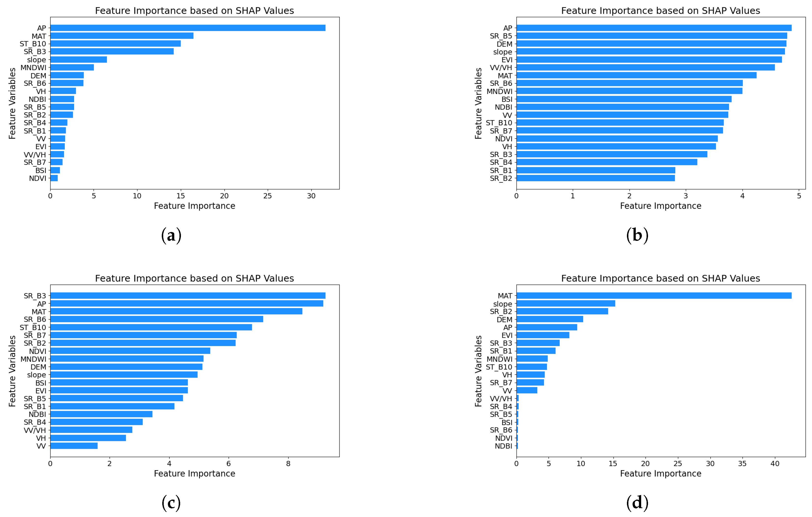
To model AGB, we trained four ML models (RF, SVR, XGBoost, and Cubist), using remote sensing-derived spectral indices, climate variables, and terrain features. Feature selection and integration of multi-dimensional environmental inputs improved model performance in capturing spatial biomass variation. To quantify each variable’s influence on model predictions, we employed SHAP values. Figure 3 shows the relative importance of predictors across models. AP consistently emerged as the most influential variable, particularly in RF and SVR, underscoring the role of macroclimate in mangrove productivity. MAT followed, while spectral indices such as NDVI, EVI, and MNDWI contributed significantly across models. DEM and slope also played notable roles, particularly in XGBoost and Cubist models. These findings are consistent with previous research on the environmental drivers of mangrove biomass [49,50,51].

3.2. Performance of Different AGB Estimation Models

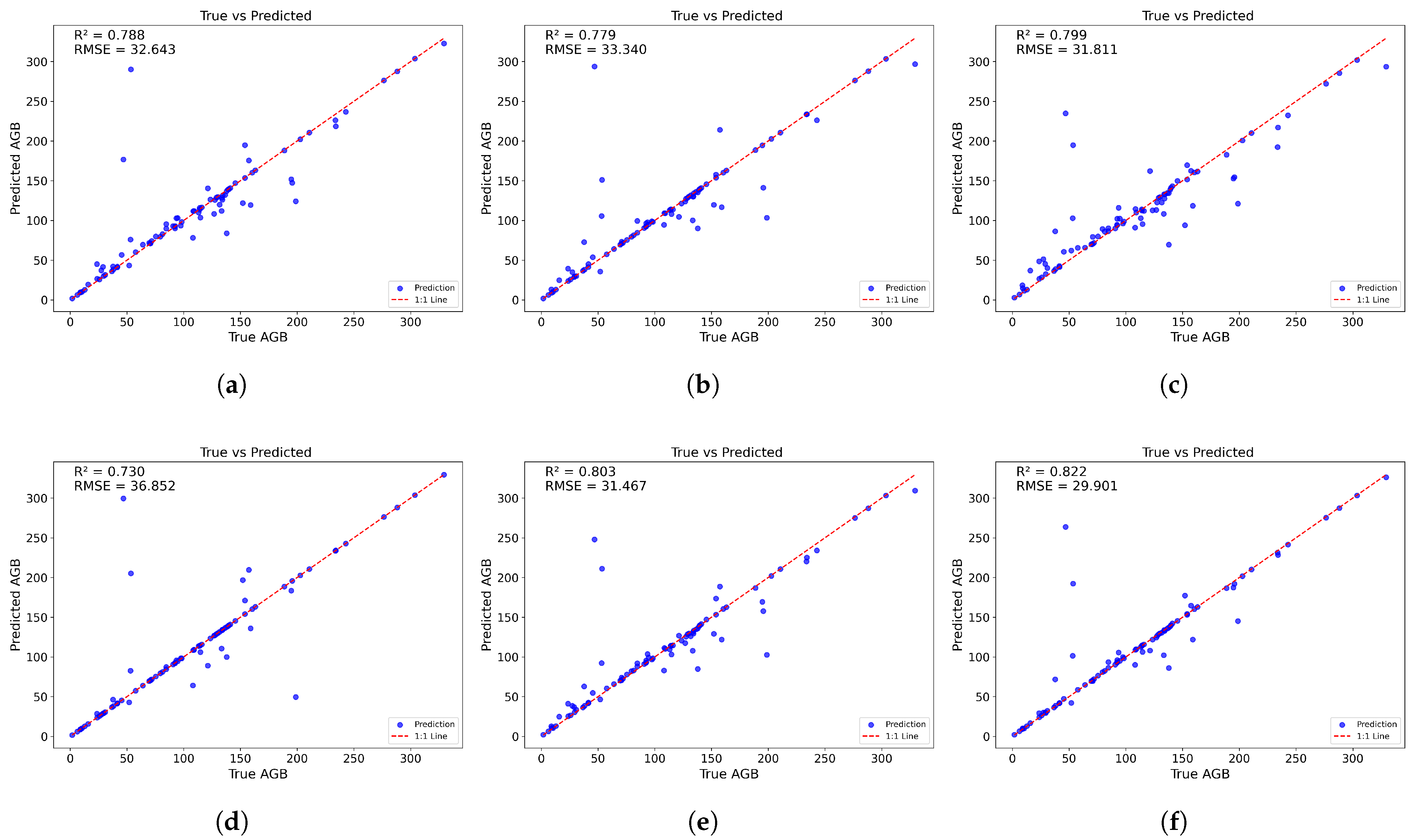
Table 1 presents the performance comparison of various AGB estimation models. When using all input variables, all four baseline ML models (RF, Cubist, SVR, and XGBoost) achieved comparable results, with R 2 values ranging from 0.73 to 0.80. Feature optimization based on SHAP values and AIC yielded modest improvements in most cases. For the RF and Cubist models, optimization led to slight reductions in RMSE and AIC, while R 2 remained unchanged. Notably, SVR performed best with all variables, while XGBoost benefited more notably from feature selection, with R 2 increasing from 0.78 to 0.80 and RMSE decreasing from 33.08 to 31.47 Mg/ha.
Building on the outputs of individual models, the ensemble-based ML-BMA method further improved prediction accuracy. It achieved an R 2 of 0.80 and an RMSE of 31.47 Mg/ha, outperforming all individual models. This demonstrates the effectiveness of BMA in leveraging the strengths of multiple learners. The proposed SAC-BA model exhibited the highest overall accuracy, as evidenced by an R 2 of 0.82 and RMSE of 29.90 Mg/ha (Figure 4), representing substantial improvements over both individual models and the ML-BMA ensemble. These results indicate that integrating spatial attention and spatial heterogeneity factors can significantly enhance the accuracy of AGB estimation.

3.3. Spatial Pattern Analysis

This study investigated the spatial heterogeneity of mangrove AGB estimation through spatial attention weights, LISA clustering, and uncertainty analysis.
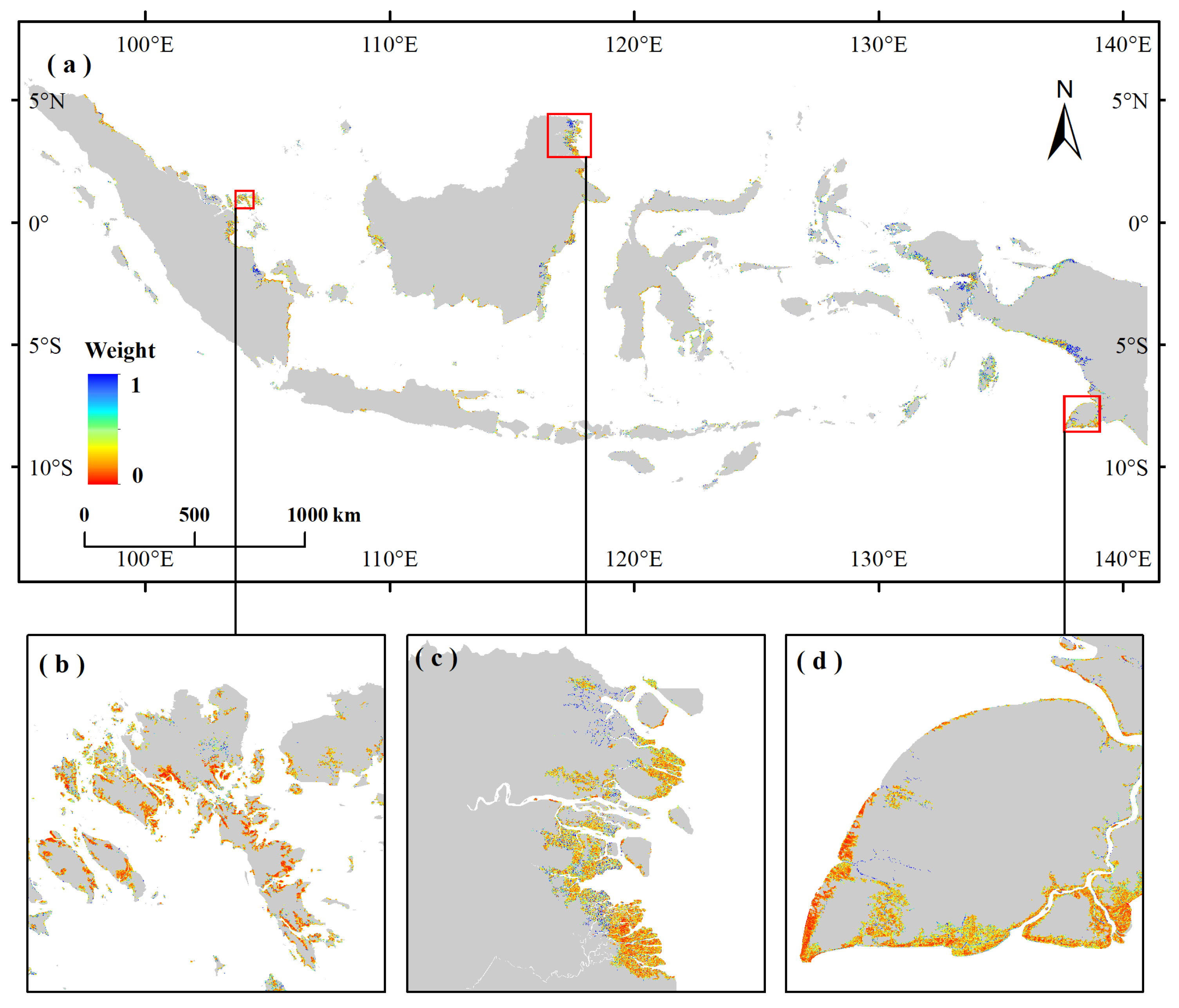
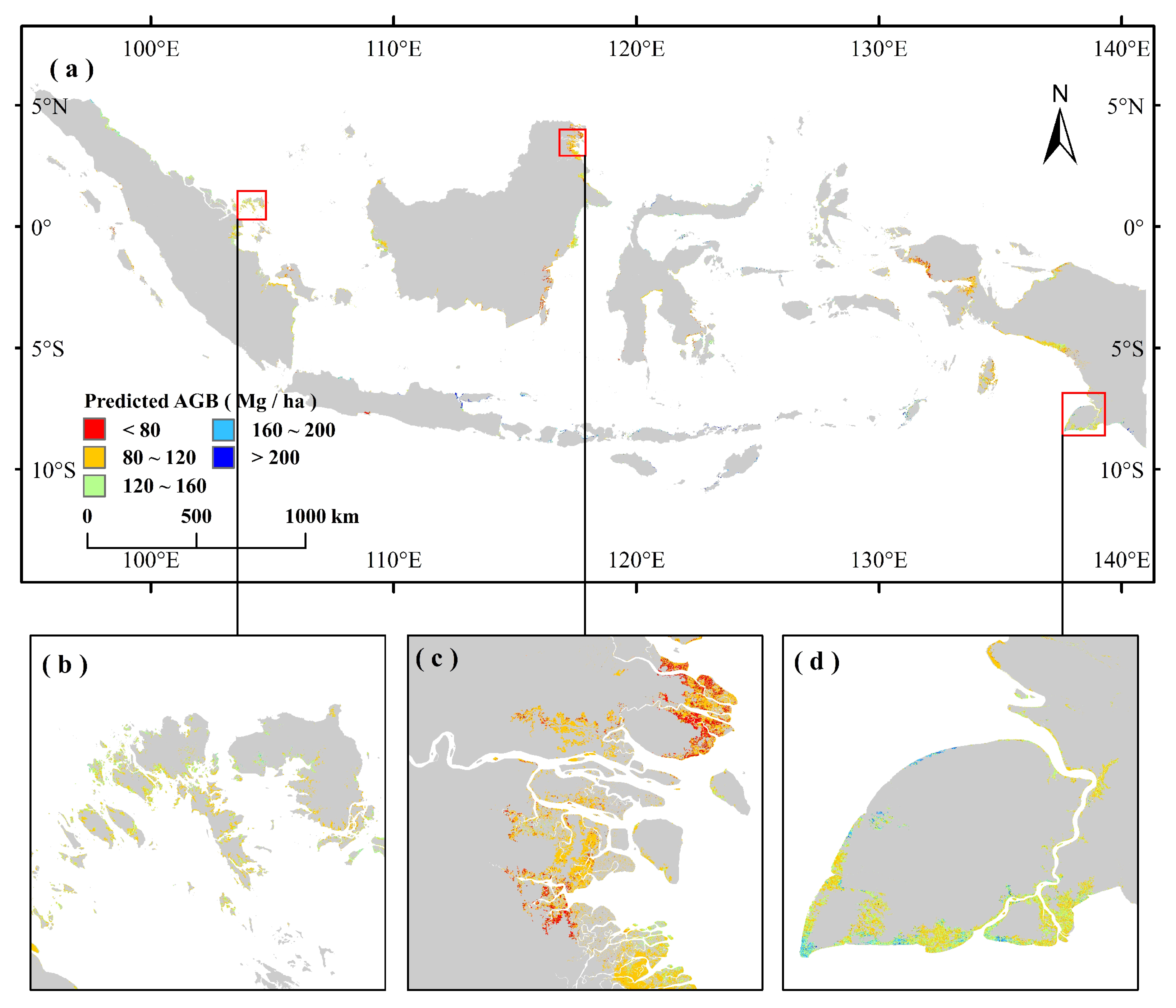
Figure 5 illustrates the spatial distribution of attention weights generated by the SAC-BA model during the AGB fusion prediction process. The color gradient from red to blue indicates the importance of each pixel, from low to high, reflecting the model’s perception and focus across different spatial regions. Overall, the attention weights display clear spatial heterogeneity across geographical areas, suggesting that the model effectively responds to variations in local representativeness and structural stability. Higher attention weights are primarily concentrated in the core mangrove zones along the coastlines, such as southern Kalimantan, western Papua, and northeastern Sumatra. These regions typically feature extensive, continuous mangrove coverage, strong structural integrity, and stable remote sensing characteristics, leading the model to assign them greater importance in the fusion process.
To further evaluate the ecological consistency of the attention mechanism in SAC-BA, we compared the spatial distribution of attention weights (Figure 5) with the Global Mangrove Soil Organic Carbon Stocks dataset, which was developed using a spatiotemporal machine learning framework [52]. Notably, high attention weights in our model were concentrated in Java, Papua Barat, Kalimantan, and the Riau region, which also exhibit higher soil organic carbon density in the global dataset. This spatial correspondence suggests that SAC-BA’s attention mechanism effectively prioritizes ecologically significant regions with high carbon storage potential. It reinforces the model’s ability to identify zones of greater ecological relevance, thus enhancing both prediction accuracy and interpretability.
In this study, the LISA clustering results used to construct the SAC-BA model were derived from the AGB predictions of the ML-BMA model. The HH and LL clusters indicate the spatial aggregation of high and low AGB values, respectively, rather than a random distribution, suggesting a strong spatial autocorrelation of mangrove AGB in the study area. In contrast, HL and LH clusters typically represent spatial edge zones or local anomalies. Compared to ML-BMA, the improved SAC-BA model showed a substantial increase in the number of HH and LL clusters, accompanied by a reduction in NS, HL, and LH clusters (as shown in Figure 6). This indicates that the SAC-BA model has a stronger capability in capturing structurally stable areas and is more effective in suppressing spatial randomness and unstable boundary regions.
Figure 7 compares the spatial details of LISA classifications across three representative regions. In Site A, both SAC-BA and ML-BMA identified extensive LL-type areas, but SAC-BA demonstrated better continuity and boundary integrity, with a notable reduction in NS zones. In Site B, ML-BMA produced a large number of HL and LH edge-type patches with mixed cluster patterns, while SAC-BA effectively reassigned many of these fragmented zones into coherent HH regions, thereby improving spatial consistency. In Site C, SAC-BA significantly reduced the extent of NS areas and enhanced the identification of HH and LL clusters, resulting in more stable and structurally coherent prediction outcomes.
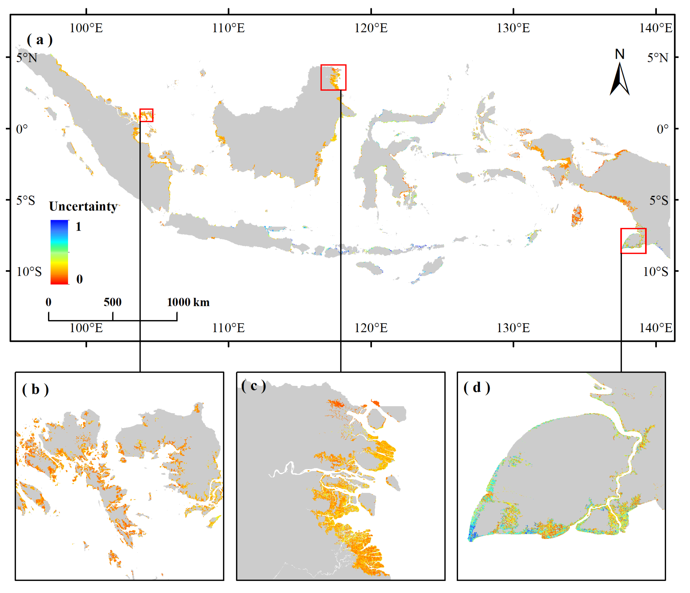
Figure 8 presents the normalized uncertainty map generated by the SAC-BA model during the mangrove AGB prediction process. This map reflects the model’s confidence levels across different regions, as well as its sensitivity to spatial factors such as sample sparsity, terrain complexity, and structural boundaries. Across the Indonesian region, uncertainty exhibits clear spatial heterogeneity. The overall trend shows lower uncertainty in core mangrove zones and large continuous areas, while higher uncertainty is observed in edge regions, fragmented island zones, estuarine intersections, and areas with frequent disturbances. This spatial pattern demonstrates that the fusion process in the SAC-BA model effectively distinguishes between high-confidence and high-risk areas, providing a solid basis for subsequent weighted optimization. Although spatial autocorrelation of residuals was not explicitly modeled during area-level aggregation, SAC-BA’s integration of LISA-based structural constraints and spatial attention mechanisms helps suppress noise propagation and over-smoothing, particularly along ecological boundaries and high-variance zones.

3.4. The Spatial Distribution of AGB

To assess model performance in mangrove AGB estimation, this study compared four traditional ML models (RF, SVR, XGBoost, Cubist) and two ensemble models (ML-BMA, SAC-BA). RF and Cubist produced smooth spatial outputs (9.56–290.96 and 5.12–299.71 Mg/ha, respectively), but showed fragmentation in edge and complex terrain regions. SVR (10.46–282.46 Mg/ha) was stable but conservative, underestimating high-AGB zones. XGBoost (3.62–273.33 Mg/ha) captured some extremes but displayed localized anomalies and lower average predictions.
ML-BMA incorporated uncertainty in its ensemble process, producing a wider AGB range (5.12–299.65 Mg/ha) but remained conservative in structure. The proposed SAC-BA model integrated uncertainty, spatial attention, and LISA-based constraints, yielding more balanced and realistic spatial patterns (11.38–291.65 Mg/ha, mean = 103.20 Mg/ha, total = 217.17 × 10 6 Mg) (Figure 9). It effectively responded to high-value zones and edge transitions while avoiding over-smoothing or noise amplification. To quantify national-scale uncertainty, we aggregated the standard deviation outputs from the ensemble predictions of SAC-BA. The resulting uncertainty was ±1.17 × 10 7 Mg, equivalent to 5.4% of the total AGB. While the pixel-level uncertainty map is visualized as a relative percentage in Figure 8, the area-level estimate was derived from the absolute uncertainty values.
Regionally, Papua exhibited the highest AGB (68.81 × 10 5 Mg), followed by Kalimantan (68.13 × 10 5 Mg). Despite their smaller, fragmented patches, Java and Sumatra also contributed meaningfully, highlighting the ecological value of conserving even minor mangrove areas.
In addition, three representative regions in Indonesia were selected for comparative analysis, as illustrated in Figure 10. The AGB distribution maps generated by the SAC-BA method reveal clearer spatial variation patterns that align more closely with the actual mangrove distribution. Across all three selected sites, the SAC-BA model effectively balances spatial smoothness and sensitivity to extreme values, successfully identifying continuous high-AGB zones. In peripheral areas, the model demonstrates distinct transitional gradients, and the prediction results exhibit strong spatial coherence.

4. Discussion

4.1. Comparison with Historical AGB Maps

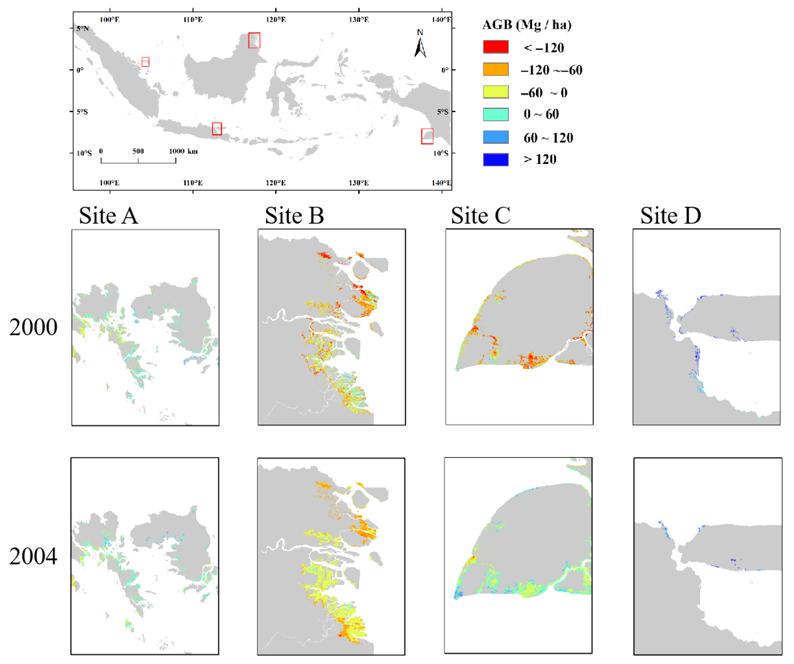
To further assess the ecological plausibility of our model results, we compared the 2017 AGB map based on SAC-BA with the global mangrove AGB products published by Simard et al. [53] in 2000 and Hu et al. [31] in 2004. Figure 11 illustrates the spatial differences among four representative sites in Indonesia. Red areas indicate increased AGB, while blue areas indicate decreased AGB. In regions such as Kalimantan (Site B) and Sumatra (Site C), our results align with historically high biomass areas, indicating that SAC-BA can accurately capture spatial biomass patterns over time. Although this comparison is not based on direct ground observations, the consistency in temporal trends provides valuable validation and further reinforces the spatial credibility of our predictions.
Variations in AGB estimates across previous studies can be largely attributed to differences in data sources, modeling strategies, and spatial resolutions. For example, Mitchard et al. [54] compared two pan-tropical biomass maps based on LiDAR-derived canopy height, but calibrated with different field data and modeling approaches, revealing substantial spatial discrepancies despite similar global totals. Baccini et al. [55] used LiDAR, optical imagery, and climate data to build a linear regression model for tropical forest carbon estimation and Avitabile et al. [56] fused multiple existing products to reduce bias. These methodological differences result in inconsistencies in biomass magnitude and spatial patterns. Bouvet et al. [57] utilized ALOS PALSAR L-band SAR data and Bayesian inversion to produce a 25 m resolution biomass map of African savannas.
Compared with these datasets, our SAC-BA model leverages spatial autocorrelation, model uncertainty, and multi-source predictors to produce more balanced and ecologically coherent outputs. While minor differences in absolute values remain, the predicted spatial distribution patterns align well with known mangrove zones, especially in Sumatra, Borneo, and Papua.

4.2. Novelty and Advantages of the SAC-BA Method

The proposed SAC-BA framework provides a novel and robust approach for estimating AGB in mangrove ecosystems by integrating spatial attention mechanisms with Bayesian model averaging. Compared with conventional ensemble methods, such as simple averaging or traditional BMA [47], SAC-BA explicitly incorporates spatial structure information into the fusion process through LISA-based spatial autocorrelation and local attention mechanisms. This design addresses the common challenge of spatial fragmentation in AGB mapping and enhances prediction consistency across heterogeneous landscapes.
Recent studies have employed BMA for biomass estimation in terrestrial ecosystems. For example, Zeng et al. [58] applied BMA combined with machine learning to estimate grassland AGB in the Three-River Headwater Region of China. However, their framework did not explicitly consider spatial heterogeneity or spatial dependence in model fusion, limiting its effectiveness in complex landscapes. In contrast, SAC-BA integrates both spatial autocorrelation and uncertainty-aware weighting, offering a more spatially coherent and ecologically interpretable mapping framework, particularly suited to fragmented coastal ecosystems like mangroves.
SAC-BA offers distinct advantages over machine learning-based approaches commonly applied in mangrove AGB estimation. Pham et al. [59] utilized XGBoost with Sentinel-2 and ALOS-2 PALSAR-2 datasets to estimate mangrove AGB but did not explicitly model spatial relationships, which can lead to boundary artifacts and spatial inconsistency in heterogeneous regions. Similarly, Basyuni et al. [60] focused on UAV-based regression models at the local scale, achieving fine resolution but lacking scalability and transferability for national-scale AGB monitoring. Compared with these approaches, SAC-BA combines spatial attention, spatial autocorrelation, and probabilistic fusion to enhance prediction accuracy and spatial generalization across large and complex mangrove landscapes.
In addition, the spatial attention mechanism embedded within SAC-BA prioritizes ecologically significant areas, such as dense mangrove cores, ensuring that these regions receive greater modeling focus during prediction. This spatially adaptive mechanism is consistent with the insights presented by Hu [31] and Twomey [61], which underscore spatial heterogeneity as a key factor in global mangrove biomass estimation. However, SAC-BA further advances these ideas by offering higher spatial resolution outputs with reduced uncertainty and enhanced boundary consistency. Collectively, SAC-BA provides a scalable, robust, and interpretable framework for regional to national-scale mangrove AGB estimation and blue carbon monitoring.

4.3. Limitations of the Current Study

Although our mangrove AGB map for Indonesia demonstrates improved accuracy over previous maps, it still shares limitations common to earlier studies, both in terms of data and methodology.
The primary limitation lies in the inherent uncertainty of ground-based AGB measurements, which arises from errors in estimation methods, such as inaccuracies in measurement techniques and allometric models, as well as geographic location errors. These sources of uncertainty cannot be fully eliminated, and their impact on results is difficult to assess. This is particularly problematic when using generalized allometric models or conversion factors, which overlook variations in species composition, environmental factors, or climate. To mitigate this uncertainty, adopting localized or species-specific AGB estimation methods and enhancing the integration of remote sensing data during mapping can help reduce errors from ground-based measurements.
The second limitation arises from the time mismatch between ground measurements and remote sensing data, which can introduce uncertainty into the predictive models. The ground-based data we gathered was collected between 2016 and 2019, with a concentration in 2017, while the Landsat 8 and Sentinel-1 data employed in our study were also from 2017. However, the exact sampling year for many plots is not recorded, making it difficult to align the ground data with the satellite data used for model fitting. If we had restricted the analysis to data from 2017, the sample size would have been insufficient for effective model training.
In addition, although we aggregated pixel-level uncertainties derived from the ensemble predictions of SAC-BA to estimate national-scale uncertainty (±1.966 × 10 7 Mg, equivalent to 8.3% of the total AGB), this approach assumes pixel-level uncertainties are independent and does not explicitly account for the spatial autocorrelation of errors. Consequently, the aggregated uncertainty may be underestimated, as spatially correlated residuals can lead to compounded uncertainty when scaling up. Future studies could incorporate geostatistical methods or spatial hierarchical models to more rigorously account for spatial dependence in uncertainty propagation.

4.4. Further Improvement of Mangrove AGB Estimation

One potential approach to enhance AGB estimation is the development of stratified models tailored to different mangrove species groups. Mangrove ecosystems consist of several species, such as Aegialitis, Rhizophora, and Avicennia, each of which exhibits distinct growth characteristics, ecological requirements, and biomass accumulation patterns. As a result, using a single model for AGB estimation may fail to fully account for the variations between species. By creating stratified models that are specific to the characteristics of each mangrove species, we can obtain more accurate AGB estimates that reflect the unique traits and ecological dynamics of each species.
It is important to note that Twomey et al. [61] have developed a global dataset on mangrove species distribution, which significantly aids in improving AGB estimation. This dataset provides spatial information on the distribution of mangrove species worldwide, helping to identify the areas where different species are found and their ecological characteristics. By integrating this dataset, we can develop more accurate stratified models based on the distribution and ecological adaptability of each species, thereby enhancing the precision of AGB estimation.
Moreover, considering the ecological diversity of mangrove species across different regions, adaptive models could enhance AGB predictions by incorporating regional factors such as climate, soil types, and hydrological conditions. This approach would not only improve biomass estimation for local mangrove areas but also provide more reliable data for global assessments of mangrove carbon stocks. Ultimately, these models would deepen our understanding of the carbon storage potential of mangrove ecosystems and their responses to climate change.

5. Conclusions

Spatial quantification of mangrove AGB is essential for understanding blue carbon dynamics and informing conservation and climate mitigation strategies. In this study, we developed SAC-BA, a novel ensemble framework that integrates field-observed AGB data with multi-source remote sensing, meteorological, and topographic variables through a spatially structured and uncertainty-aware Bayesian fusion process. Unlike conventional ensemble methods, SAC-BA incorporates spatial attention weights and LISA-based constraints into Bayesian model averaging, explicitly addressing the spatial autocorrelation often observed in biomass distribution and model residuals. This integration improves both the numerical accuracy and spatial consistency of AGB predictions, particularly in heterogeneous and fragmented mangrove landscapes. The findings highlight the advantages of combining probabilistic reasoning with spatial structure modeling in ecological applications. SAC-BA offers a scalable and transferable approach for regional biomass estimation, capable of preserving fine-scale ecological patterns while minimizing uncertainty in high-risk zones.

Author Contributions

Conceptualization, X.Z. and S.Q.; methodology, X.Z.; software, X.Z.; validation, C.S., and S.Q.; formal analysis, X.Z. and Z.X.; data curation, C.S. and S.Q.; writing—original draft preparation, X.Z.; writing—review and editing, Z.X.; supervision, S.Q.; All authors have read and agreed to the published version of the manuscript.

Funding

This research was supported in part by the National Natural Science Foundation of China (42271324, 42201406), the Natural Science Foundation of Jiangsu Province (BK20221506).

Data Availability Statement

The original data presented in the study are openly available in FigShare at [https://doi.org/10.6084/m9.figshare.29400035.v1] (accessed on 7 August 2025). The GEE script used for image preprocessing and feature extraction is available at https://code.earthengine.google.com/b9121a27b2cec2a74550ec9dcd41f7be (accessed on 7 August 2025).

Conflicts of Interest

The authors declare no conflicts of interest.

Appendix A

This appendix provides supplementary tables referenced in the main text. Table A1 lists the sources and descriptions of the input data used for model construction; Table A2 presents descriptive statistics for the AGB and related predictive factors of 89 mangrove sites. These tables support the data analysis and model interpretation in Section 2.1 and Section 3.1.
Table A1. All explanatory variables used in this study.
Data NameVariable IndexVariable NameDescriptionSpatial Resolution
Sentinel-11VVRadar band with vertical10 m
transmission and vertical reception
2VHRadar band with vertical
transmission and horizontal reception
3VV/VHRatio of VV to VH bands
Landsat 84SR_B1Coastal aerosol band30 m
5SR_B2Blue band
6SR_B3Green band
7SR_B4Red band
8SR_B5Near-infrared band
9SR_B6Shortwave infrared band 1
10SR_B7Shortwave infrared band 2
11ST_B10Thermal infrared band
12BSI(SR_B6 + SR_B4 − SR_B5 − SR_B2)/
(SR_B6 + SR_B4 + SR_B5 + SR_B2)
13EVI2.5 × (SR_B5 − SR_B4)/
(SR_B5 + 6 × SR_B4 − 7.5 × SR_B2 + 1)
14MNDWI(SR_B3 − SR_B6) / (SR_B3 + SR_B6)
15NDBI(SR_B6 − SR_B5) / (SR_B6 + SR_B5)
16NDVI(SR_B5 − SR_B4) / (SR_B5 + SR_B4)
Copernicus DEM17DEMDigital elevation model30 m
18SlopeThe steepness of the terrain
Climate Research Unit19MATMean Annual temperature 0.5
20APAnnual precipitation
Table A2. Statistical analysis of AGB and predictive variables was conducted based on the 89 sample points.
MeanMaximumMinimumMedianSDCV (%)Range
AGB109.66329.361.70108.5171.2764.99327.66
AP2518.403937.101302.002631.70585.9223.272635.10
BSI−0.25−0.07−0.55−0.240.09-0.48
EVI0.340.550.080.350.1030.050.47
MAT26.9828.6824.8326.870.782.893.842
MNDWI−0.100.20−0.47−0.110.16-0.67
NDBI−0.41−0.19−0.60−0.420.08-0.37
NDVI0.470.870.110.430.2144.270.76
SR_B10.070.270.000.040.0798.320.27
SR_B20.080.270.010.050.0783.960.26
SR_B30.120.300.040.010.0655.420.26
SR_B40.100.300.010.090.0764.470.28
SR_B50.310.450.120.320.0720.880.33
SR_B60.130.210.060.130.0324.480.15
SR_B70.100.190.040.090.0438.510.15
ST_B100.871.080.280.940.1821.080.80
VH−16.14−13.22−22.66−15.412.32-9.44
VV−10.20−7.23−17.27−9.442.45-10.05
VV/VH0.610.770.520.600.069.180.25
DEM9.4726.820.508.515.5758.8026.32
slope4.3912.190.753.732.6560.3511.45

References

  1. Zhang, Y.; Zhao, M.; Cui, Q.; Fan, W.; Qi, J.; Chen, Y.; Zhang, Y.; Gao, K.; Fan, J.; Wang, G.; et al. Processes of coastal ecosystem carbon sequestration and approaches for increasing carbon sink. Sci. China Earth Sci. 2017, 60, 809–820. [Google Scholar] [CrossRef]
  2. Alongi, D.M.; Mukhopadhyay, S.K. Contribution of mangroves to coastal carbon cycling in low latitude seas. Agric. For. Meteorol. 2015, 213, 266–272. [Google Scholar] [CrossRef]
  3. Donato, D.C.; Kauffman, J.B.; Murdiyarso, D.; Kurnianto, S.; Stidham, M.; Kanninen, M. Mangroves among the most carbon-rich forests in the tropics. Nat. Geosci. 2011, 4, 293–297. [Google Scholar] [CrossRef]
  4. McLeod, E.; Chmura, G.L.; Bouillon, S.; Salm, R.; Björk, M.; Duarte, C.M.; Lovelock, C.E.; Schlesinger, W.H.; Silliman, B.R. A blueprint for blue carbon: Toward an improved understanding of the role of vegetated coastal habitats in sequestering CO2. Front. Ecol. Environ. 2011, 9, 552–560. [Google Scholar] [CrossRef]
  5. Pendleton, L.; Donato, D.C.; Murray, B.C.; Crooks, S.; Jenkins, W.A.; Sifleet, S.; Craft, C.; Fourqurean, J.W.; Kauffman, J.B.; Marbà, N.; et al. Estimating global “blue carbon” emissions from conversion and degradation of vegetated coastal ecosystems. PLoS ONE 2012, 7, e43542. [Google Scholar] [CrossRef] [PubMed]
  6. Giri, C.; Ochieng, E.; Tieszen, L.L.; Zhu, Z.; Singh, A.; Loveland, T.; Masek, J.; Duke, N. Status and distribution of mangrove forests of the world using earth observation satellite data. Glob. Ecol. Biogeogr. 2011, 20, 154–159. [Google Scholar] [CrossRef]
  7. Alongi, D.M. Carbon Cycling and Storage in Mangrove Forests. Annu. Rev. Mar. Sci. 2014, 6, 195–219. [Google Scholar] [CrossRef]
  8. Valiela, I.; Bowen, J.L.; York, J.K. Mangrove Forests: One of the World’s Threatened Major Tropical Environments: At least 35% of the area of mangrove forests has been lost in the past two decades, losses that exceed those for tropical rain forests and coral reefs, two other well-known threatened environments. Bioscience 2001, 51, 807–815. [Google Scholar] [CrossRef]
  9. Malik, A.; Jalil, A.; Arifuddin, A.; Syahmuddin, A. Biomass Carbon Stocks in the mangrove rehabilitated area of Sinjai District, South Sulawesi, Indonesia. Geogr. Environ. Sustain. 2020, 13, 32–38. [Google Scholar] [CrossRef]
  10. Murdiyarso, D.; Purbopuspito, J.; Kauffman, J.B.; Warren, M.W.; Sasmito, S.D.; Donato, D.C.; Manuri, S.; Krisnawati, H.; Taberima, S.; Kurnianto, S. The potential of Indonesian mangrove forests for global climate change mitigation. Nat. Clim. Change 2015, 5, 1089–1092. [Google Scholar] [CrossRef]
  11. Clough, B.; Scott, K. Allometric relationships for estimating above-ground biomass in six mangrove species. For. Ecol. Manag. 1989, 27, 117–127. [Google Scholar] [CrossRef]
  12. Amarasinghe, M.; Balasubramaniam, S. Net primary productivity of two mangrove forest stands on the northwestern coast of Sri Lanka. Hydrobiologia 1992, 247, 37–47. [Google Scholar] [CrossRef]
  13. Wicaksono, P. Mangrove above-ground carbon stock mapping of multi-resolution passive remote-sensing systems. Int. J. Remote Sens. 2017, 38, 1551–1578. [Google Scholar] [CrossRef]
  14. Mariano Neto, M.; da Silva, J.B.; de Brito, H.C. Carbon Stock Estimation in a Brazilian Mangrove Using Optical Satellite Data. Environ. Monit. Assess. 2023, 196, 9. [Google Scholar] [CrossRef]
  15. Hamdan, O.; Aziz, H.K.; Hasmadi, I.M. L-band ALOS PALSAR for biomass estimation of Matang Mangroves, Malaysia. Remote Sens. Environ. 2014, 155, 69–78. [Google Scholar] [CrossRef]
  16. Dashtbozorgi, F.; Hedayatiaghmashhadi, A.; Dashtbozorgi, A.; Ruiz-Agudelo, C.A.; Fürst, C.; Cirella, G.T.; Naderi, M. Ecosystem services valuation using InVEST modeling: Case from southern Iranian mangrove forests. Reg. Stud. Mar. Sci. 2023, 60, 102813. [Google Scholar] [CrossRef]
  17. Dai, Z.; Trettin, C.C.; Burton, A.J.; Tang, W.; Mangora, M.M. Estimated mangrove carbon stocks and fluxes to inform MRV for REDD+ using a process-based model. Estuar. Coast. Shelf Sci. 2023, 294, 108512. [Google Scholar] [CrossRef]
  18. Li, Z.; Zan, Q.; Yang, Q.; Zhu, D.; Chen, Y.; Yu, S. Remote estimation of mangrove aboveground carbon stock at the species level using a low-cost unmanned aerial vehicle system. Remote Sens. 2019, 11, 1018. [Google Scholar] [CrossRef]
  19. Tian, Y.; Huang, H.; Zhou, G.; Zhang, Q.; Tao, J.; Zhang, Y.; Lin, J. Aboveground mangrove biomass estimation in Beibu Gulf using machine learning and UAV remote sensing. Sci. Total Environ. 2021, 781, 146816. [Google Scholar] [CrossRef]
  20. Chave, J.; Andalo, C.; Brown, S.; Cairns, M.A.; Chambers, J.Q.; Eamus, D.; Fölster, H.; Fromard, F.; Higuchi, N.; Kira, T.; et al. Tree allometry and improved estimation of carbon stocks and balance in tropical forests. Oecologia 2005, 145, 87–99. [Google Scholar] [CrossRef]
  21. Lu, D.; Mausel, P.; Brondizio, E.; Moran, E. Change detection techniques. Int. J. Remote Sens. 2004, 25, 2365–2401. [Google Scholar] [CrossRef]
  22. Reichstein, M.; Camps-Valls, G.; Stevens, B.; Jung, M.; Denzler, J.; Carvalhais, N.; Prabhat, F. Deep learning and process understanding for data-driven Earth system science. Nature 2019, 566, 195–204. [Google Scholar] [CrossRef] [PubMed]
  23. Anselin, L. Local indicators of spatial association—LISA. Geogr. Anal. 1995, 27, 93–115. [Google Scholar] [CrossRef]
  24. Purwanto, A.D.; Wikantika, K.; Deliar, A.; Darmawan, S. Decision tree and random forest classification algorithms for mangrove forest mapping in Sembilang National Park, Indonesia. Remote Sens. 2022, 15, 16. [Google Scholar] [CrossRef]
  25. Darmawan, S.; Takeuchi, W.; Vetrita, Y.; Winarso, G.; Wikantika, K.; Sari, D. Characterization of mangrove forest types based on ALOS-PALSAR in overall Indonesian archipelago. In IOP Conference Series: Earth and Environmental Science, Proceedings of the 7th IGRSM International Remote Sensing & GIS Conference and Exhibition; Kuala Lumpur, Malaysia, 22–23 April 2014, IOP Publishing: Bristol, UK, 2014; Volume 20, p. 012051. [Google Scholar] [CrossRef]
  26. Bunting, P.; Rosenqvist, A.; Lucas, R.M.; Rebelo, L.M.; Hilarides, L.; Thomas, N.; Hardy, A.; Itoh, T.; Shimada, M.; Finlayson, C.M. The global mangrove watch—A new 2010 global baseline of mangrove extent. Remote Sensing 2018, 10, 1669. [Google Scholar] [CrossRef]
  27. Suwignyo, R.A.; Ulqodry, T.Z.; Sarno, S.; Miyakawa, H.; Tatang, T. Mangrove plant condition in the Greenbelt area of Banyuasin Peninsula, Sembilang National Park, South Sumatra, Indonesia and its restoration plan. Chiang Mai Univ. J. Nat. Sci. 2012, 11, 123–134. [Google Scholar]
  28. Arifanti, V.B.; Kauffman, J.B.; Subarno; Ilman, M.; Tosiani, A.; Novita, N. Contributions of mangrove conservation and restoration to climate change mitigation in Indonesia. Glob. Change Biol. 2022, 28, 4523–4538. [Google Scholar] [CrossRef]
  29. Hutchison, J.; Manica, A.; Swetnam, R.; Balmford, A.; Spalding, M. Predicting global patterns in mangrove forest biomass. Conserv. Lett. 2014, 7, 233–240. [Google Scholar] [CrossRef]
  30. Fatoyinbo, T.E.; Simard, M. Height and biomass of mangroves in Africa from ICESat/GLAS and SRTM. Int. J. Remote Sens. 2013, 34, 668–681. [Google Scholar] [CrossRef]
  31. Hu, T.; Zhang, Y.; Su, Y.; Zheng, Y.; Lin, G.; Guo, Q. Mapping the global mangrove forest aboveground biomass using multisource remote sensing data. Remote Sens. 2020, 12, 1690. [Google Scholar] [CrossRef]
  32. Goïta, K.; Mouloungou, J.; Bénié, G.B. Estimation of aboveground biomass and carbon in a tropical rain forest in Gabon using remote sensing and GPS data. Geocarto Int. 2019, 34, 243–259. [Google Scholar] [CrossRef]
  33. Breiman, L. Random forests. Mach. Learn. 2001, 45, 5–32. [Google Scholar] [CrossRef]
  34. Ghosh, S.; Behera, M.; Jagadish, B.; Das, A.; Mishra, D. A novel approach for estimation of aboveground biomass of a carbon-rich mangrove site in India. J. Environ. Manag. 2021, 292, 112816. [Google Scholar] [CrossRef] [PubMed]
  35. Chen, T.; Guestrin, C. XGBoost: A Scalable Tree Boosting System. In Proceedings of the 22nd Acm Sigkdd International Conference on Knowledge Discovery and Data Mining, San Francisco, CA, USA, 13–17August 2016; pp. 785–794. [Google Scholar] [CrossRef]
  36. Rijal, S.S.; Pham, T.D.; Noer’Aulia, S.; Putera, M.I.; Saintilan, N. Mapping mangrove above-ground carbon using multi-source remote sensing data and machine learning approach in Loh Buaya, Komodo National Park, Indonesia. Forests 2023, 14, 94. [Google Scholar] [CrossRef]
  37. Roy, A.D.; Arachchige, P.S.P.; Watt, M.S.; Kale, A.; Davies, M.; Heng, J.E.; Daneil, R.; Galgamuwa, G.P.; Moussa, L.G.; Timsina, K.; et al. Remote sensing-based mangrove blue carbon assessment in the Asia-Pacific: A systematic review. Sci. Total Environ. 2024, 938, 173270. [Google Scholar] [CrossRef]
  38. Kimeldorf, G.S.; Wahba, G. A correspondence between Bayesian estimation on stochastic processes and smoothing by splines. Ann. Math. Stat. 1970, 41, 495–502. [Google Scholar] [CrossRef]
  39. Pham, T.D.; Yoshino, K.; Le, N.N.; Bui, D.T. Estimating aboveground biomass of a mangrove plantation on the Northern coast of Vietnam using machine learning techniques with an integration of ALOS-2 PALSAR-2 and Sentinel-2A data. Int. J. Remote Sens. 2018, 39, 7761–7788. [Google Scholar] [CrossRef]
  40. Prakash, A.J.; Behera, M.D.; Ghosh, S.M.; Das, A.; Mishra, D. A new synergistic approach for Sentinel-1 and PALSAR-2 in a machine learning framework to predict aboveground biomass of a dense mangrove forest. Ecol. Inform. 2022, 72, 101900. [Google Scholar] [CrossRef]
  41. Wang, K.; Franklin, S.E.; Guo, X.; Cattet, M. Remote sensing of ecology, biodiversity and conservation: A review from the perspective of remote sensing specialists. Sensors 2010, 10, 9647–9667. [Google Scholar] [CrossRef]
  42. Quinlan, J.R. (1992) Learning with continuous classes. In Proceedings of the 5th Australian Joint Conference on Artificial Intelligence, Hobart, Australia, 16–18 November 1992; World Scientific: Singapore, 1992; Volume 92, pp. 343–348. [CrossRef]
  43. Huang, C.; Townshend, J. A stepwise regression tree for nonlinear approximation: Applications to estimating subpixel land cover. Int. J. Remote Sens. 2003, 24, 75–90. [Google Scholar] [CrossRef]
  44. Arruda, D.L.d.; Ker, J.C.; Veloso, G.V.; Henriques, R.J.; Fernandes-Filho, E.I.; Camêlo, D.d.L.; Gomes, L.d.C.; Schaefer, C.E.G.R. Soil carbon prediction in Marajó island wetlands. Rev. Bras. CiÊNcia Solo 2024, 48, e0230162. [Google Scholar] [CrossRef]
  45. Zhang, R.; Zhou, X.; Ouyang, Z.; Avitabile, V.; Qi, J.; Chen, J.; Giannico, V. Estimating aboveground biomass in subtropical forests of China by integrating multisource remote sensing and ground data. Remote Sens. Environ. 2019, 232, 111341. [Google Scholar] [CrossRef]
  46. Duan, Q.; Ajami, N.K.; Gao, X.; Sorooshian, S. Multi-model ensemble hydrologic prediction using Bayesian model averaging. Adv. Water Resour. 2007, 30, 1371–1386. [Google Scholar] [CrossRef]
  47. Tenneson, K.; Patterson, M.S.; Mellin, T.; Nigrelli, M.; Joria, P.; Mitchell, B. Development of a regional lidar-derived above-ground biomass model with Bayesian model averaging for use in ponderosa pine and mixed conifer forests in Arizona and New Mexico, USA. Remote Sens. 2018, 10, 442. [Google Scholar] [CrossRef]
  48. Chaudhari, S.; Mithal, V.; Polatkan, G.; Ramanath, R. An attentive survey of attention models. ACM Trans. Intell. Syst. Technol. (TIST) 2021, 12, 1–32. [Google Scholar] [CrossRef]
  49. Li, X.; Yeh, A.G.o.; Wang, S.; Liu, K.; Liu, X. Estimating mangrove wetland biomass using radar remote sensing. J. Remote Sens. Beijing 2006, 10, 387. [Google Scholar]
  50. Bai, J.; Meng, Y.; Gou, R.; Lyu, J.; Dai, Z.; Diao, X.; Zhang, H.; Luo, Y.; Zhu, X.; Lin, G. Mangrove diversity enhances plant biomass production and carbon storage in Hainan island, China. Funct. Ecol. 2021, 35, 774–786. [Google Scholar] [CrossRef]
  51. Purwanto, A.D.; Wikantika, K.; Deliar, A.; Darmawan, S.; Harto, A.B.; Khomarudin, M.R.; Ardli, E.R. Improving the accuracy of mangrove forest mapping using sentinel image and developed classification algorithm based on machine learning. J. Spat. Sci. 2024, 69, 1019–1045. [Google Scholar] [CrossRef]
  52. Maxwell, T.L.; Hengl, T.; Parente, L.L.; Minarik, R.; Worthington, T.A.; Bunting, P.; Smart, L.S.; Spalding, M.D.; Landis, E. Global mangrove soil organic carbon stocks dataset at 30 m resolution for the year 2020 based on spatiotemporal predictive machine learning. Data Brief 2023, 50, 109621. [Google Scholar] [CrossRef]
  53. Simard, M.; Fatoyinbo, L.; Smetanka, C.; Rivera-Monroy, V.H.; Castañeda-Moya, E.; Thomas, N.; Van der Stocken, T. Mangrove canopy height globally related to precipitation, temperature and cyclone frequency. Nat. Geosci. 2019, 12, 40–45. [Google Scholar] [CrossRef]
  54. Mitchard, E.T.; Saatchi, S.S.; Baccini, A.; Asner, G.P.; Goetz, S.J.; Harris, N.L.; Brown, S. Uncertainty in the spatial distribution of tropical forest biomass: A comparison of pan-tropical maps. Carbon Balance Manag. 2013, 8, 10. [Google Scholar] [CrossRef] [PubMed]
  55. Baccini, A.; Goetz, S.J.; Walker, W.; Laporte, N.; Sun, M.; Sulla-Menashe, D.; Hackler, J.; Beck, P.; Dubayah, R.; Friedl, M.; et al. Estimated carbon dioxide emissions from tropical deforestation improved by carbon-density maps. Nat. Clim. Change 2012, 2, 182–185. [Google Scholar] [CrossRef]
  56. Avitabile, V.; Herold, M.; Heuvelink, G.B.; Lewis, S.L.; Phillips, O.L.; Asner, G.P.; Armston, J.; Ashton, P.S.; Banin, L.; Bayol, N.; et al. An integrated pan-tropical biomass map using multiple reference datasets. Glob. Change Biol. 2016, 22, 1406–1420. [Google Scholar] [CrossRef]
  57. Bouvet, A.; Mermoz, S.; Le Toan, T.; Villard, L.; Mathieu, R.; Naidoo, L.; Asner, G.P. An above-ground biomass map of African savannahs and woodlands at 25 m resolution derived from ALOS PALSAR. Remote Sens. Environ. 2018, 206, 156–173. [Google Scholar] [CrossRef]
  58. Zeng, N.; Ren, X.; He, H.; Zhang, L.; Li, P.; Niu, Z. Estimating the grassland aboveground biomass in the Three-River Headwater Region of China using machine learning and Bayesian model averaging. Environ. Res. Lett. 2021, 16, 114020. [Google Scholar] [CrossRef]
  59. Pham, T.D.; Le, N.N.; Ha, N.T.; Nguyen, L.V.; Xia, J.; Yokoya, N.; To, T.T.; Trinh, H.X.; Kieu, L.Q.; Takeuchi, W. Estimating mangrove above-ground biomass using extreme gradient boosting decision trees algorithm with fused sentinel-2 and ALOS-2 PALSAR-2 data in can Gio biosphere reserve, Vietnam. Remote Sens. 2020, 12, 777. [Google Scholar] [CrossRef]
  60. Basyuni, M.; Mubaraq, A.; Amelia, R.; Wirasatriya, A.; Iryanthony, S.B.; Slamet, B.; Al Mustaniroh, S.S.; Pradisty, N.A.; Sidik, F.; Hanintyo, R.; et al. Mangrove aboveground biomass estimation using UAV imagery and a constructed height model in Budeng–Perancak, Bali, Indonesia. Ecol. Inform. 2025, 86, 103037. [Google Scholar] [CrossRef]
  61. Twomey, A.; Lovelock, C. Global spatial dataset of mangrove genus distribution in seaward and riverine margins. Sci. Data 2024, 11, 306. [Google Scholar] [CrossRef] [PubMed]
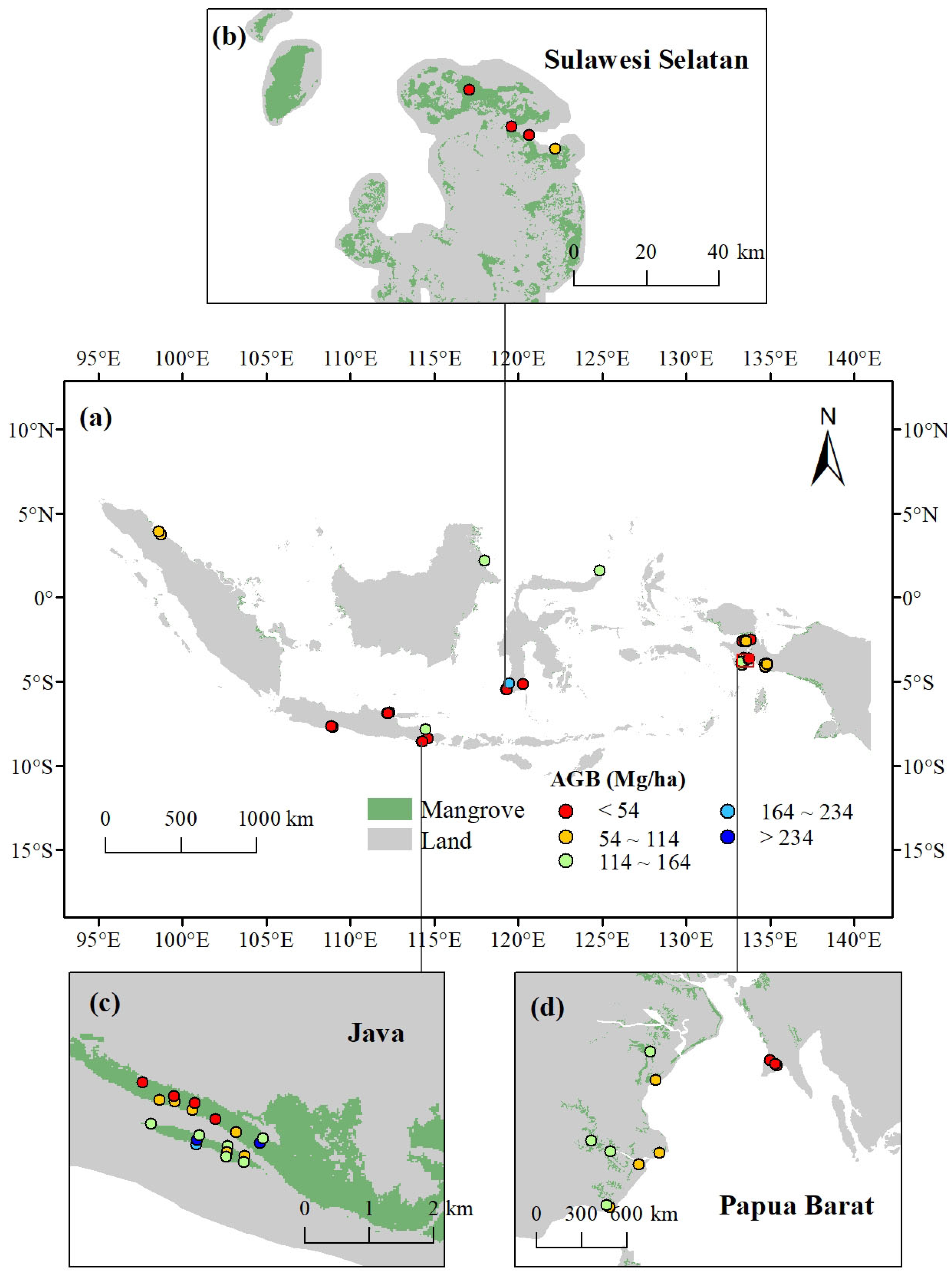
Figure 1. Study area of Indonesia and observation site data. (a) Across Indonesia, (b) zoomed in on Sulawesi Selatan, (c) zoomed in on Java, and (d) zoomed in on Papua Barat.
Forests 16 01296 g001
Figure 2. The flowchart of the Spatial Attention Coupled Bayesian Aggregator (SAC-BA) for AGB estimation.
Forests 16 01296 g002
Figure 3. Using SHAP to visualize the feature importance of the four ML models. (a) RF, (b) SVR, (c) XGBoost, and (d) Cubist.
Forests 16 01296 g003
Figure 4. Scatter plots of the observed and predicted values. (a) RF, (b) SVR, (c) XGBoost, (d) Cubist, (e) ML-BMA, and (f) SAC-BA.
Forests 16 01296 g004
Figure 5. Spatial distribution of attentional weights. (a) Across Indonesia, (b) zoomed in on Sumatra, (c) zoomed in on Kalimantan, and (d) zoomed in on Maluku.
Forests 16 01296 g005
Figure 6. Comparison of ML-BMA and SAC-BA model LISA classification.
Forests 16 01296 g006
Figure 7. LISA classification maps for three typical regions.
Forests 16 01296 g007
Figure 8. Mangrove AGB uncertainty normalized distribution. (a) Across Indonesia, (b) zoomed in on Sumatra, (c) zoomed in on Jawa, and (d) zoomed in on Papua.
Forests 16 01296 g008
Figure 9. Mangrove AGB distribution predicted by SAC-BA. (a) Across Indonesia, (b) zoomed in on Sumatra, (c) zoomed in on Jawa, and (d) zoomed in on Papua.
Forests 16 01296 g009
Figure 10. Mangrove distribution predicted by different methods in typical regions.
Forests 16 01296 g010
Figure 11. Comparison between SAC-BA predicted AGB in 2017 and publicly available global mangrove AGB datasets from 2000 and 2004 across four representative regions in Indonesia.
Forests 16 01296 g011
Table 1. Performance of the AGB estimation models.
ModelInput VariablesTrainingValidationAIC
R 2 RMSE R 2 RMSE
RFAll features0.8828.610.7933.13129.27
Optimized features0.8927.860.7932.64129.02
CubistAll features0.8926.070.7336.86124.67
Optimized features0.9025.060.7336.85123.01
SVRAll features0.8623.030.7833.34126.66
Optimized features
XGBoostAll features0.8721.520.7833.08132.77
Optimized features0.8826.070.8031.81132.22
ML-BMA0.8925.380.8031.47
SAC-BA0.9021.080.8229.90
Disclaimer/Publisher’s Note: The statements, opinions and data contained in all publications are solely those of the individual author(s) and contributor(s) and not of MDPI and/or the editor(s). MDPI and/or the editor(s) disclaim responsibility for any injury to people or property resulting from any ideas, methods, instructions or products referred to in the content.