Evaluating Forest Canopy Structures and Leaf Area Index Using a Five-Band Depth Image Sensor

Abstract

The objective of the study was to develop and validate a ground-based method using a depth image sensor equipped with depth, visible red, green, blue (RGB), and near-infrared bands to measure the leaf area index (LAI) based on the relative illuminance of foliage only. The method was applied in a Itajii chinkapin (Castanopsis sieboldii (Makino) Hatus. ex T.Yamaz. & Mashiba )forest in Aichi Prefecture, Japan, and validated by comparing estimates with conventional methods (LAI-2200 and fisheye photography). To apply the 5-band sensor to actual forests, a methodology is proposed for matching the color camera and near-infrared camera in units of pixels, along with a method for widening the exposure range through multi-step camera exposure. Based on these advancements, the RGB color band, near-infrared band, and depth band are converted into several physical properties. Employing these properties, each pixel of the canopy image is classified into upper foliage, lower foliage, sky, and non-assimilated parts (stems and branches). Subsequently, the LAI is calculated using the gap-fraction method, which is based on the relative illuminance of the foliage. In comparison with existing indirect LAI estimations, this technique enabled the distinction between upper and lower canopy layers and the exclusion of non-assimilated parts. The findings indicate that the plant area index (PAI) ranged from 2.23 to 3.68 m² m⁻², representing an increase from 33% to 34% compared to the LAI calculated after excluding non-assimilating parts. The findings of this study underscore the necessity of distinguishing non-assimilated components in the estimation of LAI. The PAI estimates derived from the depth image sensor exhibited moderate to strong agreement with the LAI-2200, contingent upon canopy rings (R² = 0.48–0.98), thereby substantiating the reliability of the system’s performance. The developed approaches also permit the evaluation of the distributions of leaves and branches at various heights from the ground surface to the top of the canopy. The novel LAI measurement method developed in this study has the potential to provide precise, reliable foundational data to support research in ecology and hydrology related to complex tree structures.

1. Introduction

The forest canopy plays a critical role in the forest ecosystem by facilitating photosynthesis, capturing energy and regulating climate [1]. In temperate forests, canopies have been found to sequester approximately 280 g C m⁻² year⁻¹ carbon through photosynthesis, thereby mitigating climate change [2]. Scotch pine canopies (Pinus sylvestris) maintained year-round photosynthesis and leaf retention even in winter in northern Scandinavia [3]. The leaves of temperate deciduous broadleaf trees, such as red maple (Acer rubrum) and river birch (Betula nigra), can effectively capture light during short growing seasons compared to evergreen conifers, such as eastern red cedar (Juniperus virginiana) and jack pine (Pinus banksiana) species [4]. Forest canopies can regulate the microclimate, leading to a reduction in daily maximum air temperatures by 5.1 °C (mean: 1.8 °C) based on long-term meteorological data collected inside and outside 14 distinct forest ecosystems [5]. Canopies also reduce wind speed by 80% and regulate internal forest micrometeorological conditions [6].

The leaf area index (LAI) is a key metric for assessing forest canopy conditions [7] and is defined as the amount of leaf area per unit of ground surface area [7,8]. A related metric is the plant area index (PAI), which is the total plant area per unit of ground surface area, including leaves and non-assimilating components, such as branches and stems [9]. Therefore, PAI can be expressed as the sum of LAI and woody area index (WAI), where the WAI accounts for the woody parts of the vegetation such as stems and branches. Various studies have shown that LAI is linked to exchanges of energy, water, and gases between the canopy and the atmosphere [10]. For instance, the mean interception loss decreased from 17.9% to 9.4% as the LAI of Robinia pseudoacacia plots decreased from 2.66 to 0.33 m² m⁻² in a semiarid region of the Loess Plateau in China [11]. In Brant’s oak forests (i.e., Mt. Atlas mastic tree, Pistacia atlantica; Montpellier maple, Acer monspessulanum subsp. cinerascens; Hawthorn, Crataegus azarolus) in the Dalab region of Iran, canopy interception decreased from 30.4% during the leafed period (LAI: 0.49 m² m⁻²) to 13.9% during the leafless period (WAI: 0.49 m² m⁻²) [12]. The ratio of stand transpiration to potential evapotranspiration increased from 20% to 90% in the sessile oak stand (Quercus petraea) as LAI changed from 1.0 to 5.2 m² m⁻² in the Champenoux Forest in France [13]. Evapotranspiration decreased from 357 mm to 334 mm as the LAI decreased from 4.2 to 2.0 m² m⁻² in Prince Rupprecht’s larch (Larix principis-rupprechtii) plantations of Diediegou, China [14]. In a black spruce (Picea mariana) stand near Fairbanks, Alaska, USA, as LAI increased from 1.1 to 4.6 m² m⁻², the average net canopy assimilation increased from 800 g CO₂ m⁻² yr⁻¹ to 1814 g CO₂ m⁻² yr⁻¹ [15].

Various methods have been developed to estimate LAI, including direct or indirect sampling of leaves and remote sensing [16,17]. LAI values ranging from 5.1 to 10.4 m² m⁻² have been estimated for coniferous trees (red pine, Pinus resinosa; eastern white pine, Pinus strobus; European larch, Larix decidua; and Norway spruce, Picea abies) by felling ten trees of each species and collecting their foliage [18]. LAI estimates for a 70-year-old temperate deciduous forest, based on back-accumulation from litterfall, ranged from 4.90 to 7.98 m² m⁻² for species such as Japanese elm (Ulmus japonica) and Manchurian ash (Fraxinus mandshurica) [19]. Using hemispherical photography, the LAI of 17- and 54-year-old Douglas fir forests (Pseudotsuga menziesii) in Canada was estimated to be 4.7 and 5.9 m² m⁻², respectively [20]. The LAI of 37- to 90-year-old broad-leaved forests such as Turkey oak (Quercus cerris), sweet chestnut (Castanea sativa), and European beech (Fagus sylvatica) in Italy was estimated to be between 1.8 and 5.8 m² m⁻² using the LAI-2000 [21]. Using terrestrial laser scanning (TLS), the leaf area index (LAI) was found to be 1.14 m² m⁻² for black locust (Robinia pseudoacacia) forests in Fangshan District, Beijing, China [22]. Traditional approaches often include woody components such as branches and stems in the canopy data, which can lead to the overestimation of leaf area [23]. Hemispherical photography tends to considerably overestimate actual leaf area index (LAI), with estimated values ranging from 1.5 to 3 times higher than the measured LAI, depending on thresholding and view angle settings [24]. In essence, these indirect methods measure PAI rather than the true LAI.

Accurately assessing leaf area index (LAI) in forest landscapes requires considering the vertical and lateral distribution of leaves within forest structures, as well as non-assimilative parts such as branches and stems [25]. Temperate forests are complex ecosystems consisting of diverse trees, shrubs, herbs, and mosses arranged in distinct vertical layers from the tall tree canopy to the ground, and this complex layering is more prominent in natural forests than in plantations [26,27]. For example, the temperate forest in Korea’s Gwangneung has layers consisting of over 16 m in the upper layer (Jolcham oak, Quercus serrata), around 16 m in the middle layer (loose-flower hornbeam, Carpinus laxiflora), and approximately 4 m in the lower layer (i.e., loose-flower hornbeam, Carpinus laxiflora; hornbeam, Carpinus cordata; Japanese snowbell, Styrax japonica) [28]. The incorporation of non-assimilative components into these intricate structures has the potential to result in an overestimation of LAI. The woody area index (WAI) has been shown to comprise approximately 11% of the plant area index (PAI = 5.95 ± 0.4 m² m⁻²) as determined through destructive sampling in a flux-tower study [29]. However, the majority of remote sensing methods are incapable of distinguishing between branches, stems, and foliage. To address this challenge, an integrated hardware–software system for ground-based LAI measurement was developed. The objectives of this study were to (1) estimate canopy structure and separate branches and stems from foliage in order to accurately obtain LAI, and (2) compare new and contemporary methods of estimating LAI. This study provides reliable data that enable precise evaluations of forest ecosystems and the comprehension of intricate hydrological and ecological processes in forested landscapes.

2. Materials and Methods

2.1. Study Area and Field Measurement

The study was conducted in a broadleaf forest in the Aichi Prefecture Forest Park (468 ha), Nagoya, Japan (35°13′59.4″ N, 137°2′16.2″ E at an altitude of 73.6 m) (Figure 1). The climate in this area is temperate with 1579 mm of mean annual precipitation and 16.2 °C mean annual temperature (based on AMeDAS data from 1991 to 2020 for Nagoya City, which is located 15 km from the study site) [30]. High precipitation occurs from June to September, reaching 1085 mm per month (55%). The area is covered by a 60- to 70-year-old secondary forest consisting of Japanese chinquapin (Castanopsis cuspidata), Itajii chinkapin (Castanopsis sieboldii), blue Japanese oak (Quercus glauca), and bamboo-leaf oak (Quercus myrsinifolia) [31]. Dominant shrub species include Japanese eurya (Eurya japonica), Japanese aralia (Dendropanax trifidus), and Japanese camellia (Camellia japonica). Additionally, autumn fern (Dryopteris erythrosora), Asiatic jasmine (Trachelospermum asiaticum), and dwarf lilyturf (Ophiopogon japonicus var. umbrosus) cover the understory vegetation.

A 15 m × 30 m plot was established to measure canopy structures (Figure 1d). A plot size of 15 m × 30 m was selected to adequately capture the spatial variability of canopy gaps and vertical forest structure, thereby ensuring a representative characterization of canopy conditions in broadleaf forests. This plot dimension aligns with those employed in previous studies targeting similar forest types [32,33], and prior research has demonstrated that relatively small, strategically positioned plots can effectively detect canopy and phenological variability in structurally heterogeneous forests [34]. The area is covered by 34 Itajii chinkapin (Castanopsis sieboldii (Makino) Hatus. ex T.Yamaz. & Mashiba) trees with a density of 756 trees/ha. The diameter of breast height (DBH) ranged from 18.2 to 56.7 cm, with a mean of 35.2 cm (SD: 6.5 cm). The upper and lower canopy layers in the study plot were primarily composed of Itajii chinkapin (Castanopsis sieboldii). The upper canopy height generally ranged from 17 to 25 m, while the lower canopy was typically less than 10 m (approximately 7 to 8 m; Table S1, Supplementary Materials). Additionally, the understory vegetation primarily consists of shrubs such as Japanese cinnamon (Cinnamomum yabunikkei) and Japanese camellia (Camellia japonica), ranging from 3 to 6 m in height.

Nine measurement points (A1–A9) were selected within the plot, with distances ranging from 3 to 8 m. We used a pocket-sized depth image sensor (Intel Real Sense D455; Intel Corporation) [35], which consists of RGB, near-infrared, and depth sensors. The platform was located at 1.1 to 1.4 m height from ground surface using a tripod. Data were obtained five times within 100 s with five different exposure levels (near-infrared images: 50, 100, 200, 400, and automatic setting; RGB images: 1, 2, 4, 9, and 19). Both the color and near-infrared images can be obtained at a resolution of 1280 × 720 pixels and frame rate of 30 frames per second. The field of view (FOV) of the color image was 87° at the horizontal direction and 58° at the vertical direction, while FOV of the infrared ranged from 90° at the horizontal direction to 65° at the vertical direction. According to the specification, the depth image by the sensor is obtained from 0.4 m to nearly 10 m, while our initial test revealed that distances up to 20 m can be detected. Depth images can be overlaid pixel-by-pixel with RGB and near-infrared images at the same resolution. Maximum and minimum FOV values became ±3 degrees, which corresponded to 3 to 5% of FOV (up to 40 pixels). The deviation between RGB and near-infrared images was calibrated for matching images (Supplementary Materials).

In addition to depth image sensor measurements, the LAI-2200 Plant Canopy Analyzer [36,37] and a fish-eye camera were also used. Both LAI-2200 and fish-eye photos were taken at 1.1 to 1.4 m height same as the depth image sensor. The LAI-2200 calculates the plant area index (PAI) by collecting radiation data using a fish-eye optical sensor with five concentric rings, each capturing light at different zenith angles (ring 1: 0–12.3°; ring 2: 16.7–28.6°; ring 3: 32.4–43.4°; ring 4: 47.3–58.1°; and ring 5: 62.3–74.1°) [36]. The LAI-2200 analyzes optical thickness across these angles at 7°, 23°, 38°, 53°, and 68° degrees, assuming random leaf distribution, to estimate canopy light interception and vertical light transmittance. The fish-eye images were taken using STYLUS TG-Tracker camera (Olympus, Tokyo, Japan) with mounted fish-eye lens. The maximum FOV of the fish-eye lens was 180 degrees with 3840 × 2160 resolution. In the fish-eye images of this study, white represents sunlight transmittance, while dark green indicates canopy coverage. The PAI of fish-eye images was calculated using Hemiphot.R [38]. In addition, the canopy openness and transmitted total data from the fish-eye images were calculated using the Gap Light Analyzer (GLA v2.0) [39].

Field measurements were conducted on March 30, April 21, and April 27 in 2022. The mean air temperature in these periods was 16.6, 16.3, and 20.8 °C, with mean wind speeds of 2.0, 2.0, and 3.9 m/s, respectively. On March 30, the weather was sunny with moderate cloud cover and relatively high total daily radiation (21.65 MJ/m² from the Automated Meteorological Data Acquisition System (AMeDAS), Nagoya), while radiation tended to be low on April 21 with 8.84 MJ/m² and 2 m/s wind speed (Table S2, Supplementary Materials). The weather on April 27 tended to be cloudy with relatively high wind speeds (3.9 m/s).

2.2. Depth Image Sensor Data Processing and LAI Calculation

The development of three software programs was initiated with the objective of facilitating data capture, processing, and LAI calculation using depth image sensors (Supplementary Materials). The first software-capture program records data at the measurement site, operating the sensor to capture 5-band image data of the canopy (Supplementary Materials). The software was written in the C++ programming language. The main task of the capture program is to control the camera settings and record data of visible, near-infrared, and distance images on the hard disk [40].

The second software processes the captured images and extracts physical properties, classifying pixels into sky, foliage, and unassimilated parts. The software was written in Python programming language (version 3.11.5, Anaconda distribution). Given the disparity of 58 mm between the centers of the lenses of the near-infrared and RGB images [40], a calculation was performed to determine the matching pixels of the RGB and near-infrared images [41] (Supplementary Materials). Color calibration was not conducted in this study, as Kirk et al. (2009) demonstrated that reliable LAI estimates can be obtained using red–green channel images without the need of calibration [42]. Exposure for each pixel was adjusted by expanding the brightness range, and standardized brightness was calculated for each band and exposure level (Supplementary Materials). Pixel values within the FOV are classified into sky, foliage, and unassimilated parts as follows. When the pixels with a standardized blue brightness was equal or greater than 500 and the ratio of near-infrared (standardized to exposure level 400) to the red (standardized to exposure level 19) (IR/Red ratio) was equal or less than 1.0, the pixel was identified as “sky” with a distance value.

Furthermore, pixels without distance data with an 8-bit brightness of blue were equal to or greater than 243, and pixels matching the assumption of 1000 m distance were defined as the sky without distance value, which were used to estimate the illuminance outside the forest. Then, when a pixel value with a standard blue brightness was equal or less than 500 and an IR/Red ratio was equal or less than 0.7, the pixel was classified as “non-assimilated parts”. Pixels without distance data that did not meet the conditions for classification as sky without distance value were classified as “non-matching”. Finally, pixel values that did not meet the above conditions were classified as “foliage”. Based on such classification, we finally obtained the canopy classification image.

The third software program calculates LAI based only on the relative illuminance of pixels classified as foliage (Supplementary Materials). Relative illuminance, defined as the ratio of light under the canopy to light outside the canopy [43], was calculated by comparing the blue brightness of foliage pixels to the mean brightness of sky pixels. The mean brightness of sky pixels was scaled from 0 to 100. In this study, LAI was then derived from the relative illuminance using equations proposed by Campbell & Norman (1989) [44] and Norman & Campbell (1989) [16]. Additionally, the software supports the calculation of the plant area index (PAI).

To analyze canopy structures, concentric rings representing contour lines of zenith angles were applied with the camera facing upward. Due to the narrower field of view (FOV) of the depth image sensor compared to the LAI-2200, the PAI and LAI values from the depth image sensor were calculated within three zenith angle ranges: 0.0° to 12.3°, 16.7° to 28.6°, and 32.4° to 43.4° (rings 1, 2, and 3, respectively). These ranges correspond to the FOV of the LAI-2200 (Figure S5, Supplementary Materials). The weights of these rings were adjusted following the methods described by Castro and Fetcher (1998) [45] and Barclay et al. (2000) [46]. In addition, the PAI from the LAI-2200 and fish-eye images were also calculated using these three rings to allow a reasonable comparison with the depth image sensor results.

The sensor used in this study was based on the gap fraction method as the measurement principle, and LAI was calculated using the same method as the LAI-2200. LAI was computed using the following formulas, which were developed based on the LAI-2200 theory.

$$\mathrm{L}\mathrm{A}\mathrm{I}=2{\sum }_{\mathrm{r}\mathrm{i}\mathrm{n}\mathrm{g}=1}^3\left[-{\displaystyle \frac{{\mathrm{L}\mathrm{o}\mathrm{g}}_{\mathrm{e}}\left({\mathrm{T}}_{\mathrm{r}\mathrm{i}\mathrm{n}\mathrm{g}}\right)}{{\mathrm{S}}_{\mathrm{r}\mathrm{i}\mathrm{n}\mathrm{g}}}}·{\mathrm{W}}_{\mathrm{r}\mathrm{i}\mathrm{n}\mathrm{g}}\right]$$

(1)

In Equation (1), T_ring is the brightness value of a single pixel, and W_ring is the weighting factor applied to the brightness values of the pixels. Ring indicates the concentric sensor rings of the LAI-2200 corresponding to specific zenith angle ranges. These rings cover the following angles: ring 1 (0–12.3°), ring 2 (16.7–28.6°), and ring 3 (32.4–43.4°).

Depending on the specific objective of the calculation, the settings of T_ring and W_ring in Equation (1) vary accordingly:

When estimating the PAI, which includes non-assimilating parts such as branches and trunks, the parameters are determined based on Equations (2)–(4):

$${\mathrm{T}}_{\mathrm{r}\mathrm{i}\mathrm{n}\mathrm{g}}={\displaystyle \frac{\mathrm{S}\mathrm{U}\mathrm{M}\left({\mathrm{T}}_{\mathrm{G}\mathrm{A}\mathrm{C}}\right)+\mathrm{S}\mathrm{U}\mathrm{M}\left({\mathrm{T}}_{\mathrm{U}\mathrm{p}\mathrm{p}\mathrm{e}\mathrm{r}\mathrm{F}\mathrm{o}\mathrm{l}\mathrm{i}\mathrm{a}\mathrm{g}\mathrm{e}}\right)+\mathrm{S}\mathrm{U}\mathrm{M}\left({\mathrm{T}}_{\mathrm{L}\mathrm{o}\mathrm{w}\mathrm{e}\mathrm{r}\mathrm{F}\mathrm{o}\mathrm{l}\mathrm{i}\mathrm{a}\mathrm{g}\mathrm{e}}\right)+\mathrm{S}\mathrm{U}\mathrm{M}\left({\mathrm{T}}_{\mathrm{S}\mathrm{t}\mathrm{e}\mathrm{m}\&\mathrm{B}\mathrm{r}\mathrm{a}\mathrm{n}\mathrm{c}\mathrm{h}}\right)}{{\mathrm{N}}_{\mathrm{G}\mathrm{A}\mathrm{C}}+{\mathrm{N}}_{\mathrm{U}\mathrm{p}\mathrm{p}\mathrm{e}\mathrm{r}\mathrm{F}\mathrm{o}\mathrm{l}\mathrm{i}\mathrm{a}\mathrm{g}\mathrm{e}}+{\mathrm{N}}_{\mathrm{L}\mathrm{o}\mathrm{w}\mathrm{e}\mathrm{r}\mathrm{F}\mathrm{o}\mathrm{l}\mathrm{i}\mathrm{a}\mathrm{g}\mathrm{e}}+{\mathrm{N}}_{\mathrm{S}\mathrm{t}\mathrm{e}\mathrm{m}\&\mathrm{B}\mathrm{r}\mathrm{a}\mathrm{n}\mathrm{c}\mathrm{h}}}}$$

(2)

$${\left({\mathrm{N}}_{\mathrm{A}\mathrm{L}\mathrm{L}}\right)}_{\mathrm{r}\mathrm{i}\mathrm{n}\mathrm{g}}={\mathrm{N}}_{\mathrm{G}\mathrm{A}\mathrm{C}}+{\mathrm{N}}_{\mathrm{U}\mathrm{p}\mathrm{p}\mathrm{e}\mathrm{r}\mathrm{F}\mathrm{o}\mathrm{l}\mathrm{i}\mathrm{a}\mathrm{g}\mathrm{e}}+{\mathrm{N}}_{\mathrm{L}\mathrm{o}\mathrm{w}\mathrm{e}\mathrm{r}\mathrm{F}\mathrm{o}\mathrm{l}\mathrm{i}\mathrm{a}\mathrm{g}\mathrm{e}}+{\mathrm{N}}_{\mathrm{S}\mathrm{t}\mathrm{e}\mathrm{m}\&\mathrm{B}\mathrm{r}\mathrm{a}\mathrm{n}\mathrm{c}\mathrm{h}}$$

(3)

$${\mathrm{W}}_{\mathrm{r}\mathrm{i}\mathrm{n}\mathrm{g}}={\mathrm{N}}_{\mathrm{A}\mathrm{L}\mathrm{L}}/\sum _{\mathrm{r}\mathrm{i}\mathrm{n}\mathrm{g}=1}^{\mathrm{r}\mathrm{i}\mathrm{n}\mathrm{g}=3}({\mathrm{N}}_{\mathrm{G}\mathrm{A}\mathrm{C}}+{\mathrm{N}}_{\mathrm{U}\mathrm{p}\mathrm{p}\mathrm{e}\mathrm{r}\mathrm{F}\mathrm{o}\mathrm{l}\mathrm{i}\mathrm{a}\mathrm{g}\mathrm{e}}+{\mathrm{N}}_{\mathrm{L}\mathrm{o}\mathrm{w}\mathrm{e}\mathrm{r}\mathrm{F}\mathrm{o}\mathrm{l}\mathrm{i}\mathrm{a}\mathrm{g}\mathrm{e}}+{\mathrm{N}}_{\mathrm{S}\mathrm{t}\mathrm{e}\mathrm{m}\&\mathrm{B}\mathrm{r}\mathrm{a}\mathrm{n}\mathrm{c}\mathrm{h}})$$

(4)

where SUM(T) is the total brightness value across all pixels, and N is the total number of pixels included in the calculation. GAC (gaps among crown) is the sky.

For calculating the leaf area index (LAI) by excluding non-assimilating components and considering only foliage, the parameters are based on Equations (5)–(7):

$${\mathrm{T}}_{\mathrm{r}\mathrm{i}\mathrm{n}\mathrm{g}}={\displaystyle \frac{\mathrm{S}\mathrm{U}\mathrm{M}\left({\mathrm{T}}_{\mathrm{U}\mathrm{p}\mathrm{p}\mathrm{e}\mathrm{r}\mathrm{F}\mathrm{o}\mathrm{l}\mathrm{i}\mathrm{a}\mathrm{g}\mathrm{e}}\right)+\mathrm{S}\mathrm{U}\mathrm{M}\left({\mathrm{T}}_{\mathrm{L}\mathrm{o}\mathrm{w}\mathrm{e}\mathrm{r}\mathrm{F}\mathrm{o}\mathrm{l}\mathrm{i}\mathrm{a}\mathrm{g}\mathrm{e}}\right)}{{\mathrm{N}}_{\mathrm{U}\mathrm{p}\mathrm{p}\mathrm{e}\mathrm{r}\mathrm{F}\mathrm{o}\mathrm{l}\mathrm{i}\mathrm{a}\mathrm{g}\mathrm{e}}+{\mathrm{N}}_{\mathrm{L}\mathrm{o}\mathrm{w}\mathrm{e}\mathrm{r}\mathrm{F}\mathrm{o}\mathrm{l}\mathrm{i}\mathrm{a}\mathrm{g}\mathrm{e}}}}$$

(5)

$${\left({\mathrm{N}}_{\mathrm{A}\mathrm{L}\mathrm{L}}\right)}_{\mathrm{r}\mathrm{i}\mathrm{n}\mathrm{g}}={\mathrm{N}}_{\mathrm{U}\mathrm{p}\mathrm{p}\mathrm{e}\mathrm{r}\mathrm{F}\mathrm{o}\mathrm{l}\mathrm{i}\mathrm{a}\mathrm{g}\mathrm{e}}+{\mathrm{N}}_{\mathrm{L}\mathrm{o}\mathrm{w}\mathrm{e}\mathrm{r}\mathrm{F}\mathrm{o}\mathrm{l}\mathrm{i}\mathrm{a}\mathrm{g}\mathrm{e}}$$

(6)

$${\mathrm{W}}_{\mathrm{r}\mathrm{i}\mathrm{n}\mathrm{g}}={\mathrm{N}}_{\mathrm{A}\mathrm{L}\mathrm{L}}/\sum _{\mathrm{r}\mathrm{i}\mathrm{n}\mathrm{g}=1}^{\mathrm{r}\mathrm{i}\mathrm{n}\mathrm{g}=3}({\mathrm{N}}_{\mathrm{G}\mathrm{A}\mathrm{C}}+{\mathrm{N}}_{\mathrm{U}\mathrm{p}\mathrm{p}\mathrm{e}\mathrm{r}\mathrm{F}\mathrm{o}\mathrm{l}\mathrm{i}\mathrm{a}\mathrm{g}\mathrm{e}}+{\mathrm{N}}_{\mathrm{L}\mathrm{o}\mathrm{w}\mathrm{e}\mathrm{r}\mathrm{F}\mathrm{o}\mathrm{l}\mathrm{i}\mathrm{a}\mathrm{g}\mathrm{e}}+{\mathrm{N}}_{\mathrm{S}\mathrm{t}\mathrm{e}\mathrm{m}\&\mathrm{B}\mathrm{r}\mathrm{a}\mathrm{n}\mathrm{c}\mathrm{h}})$$

(7)

To further extract the LAI of upper foliage layers, the parameters follow Equations (8)–(10):

$${\mathrm{T}}_{\mathrm{r}\mathrm{i}\mathrm{n}\mathrm{g}}={\displaystyle \frac{\mathrm{S}\mathrm{U}\mathrm{M}\left({\mathrm{T}}_{\mathrm{U}\mathrm{p}\mathrm{p}\mathrm{e}\mathrm{r}\mathrm{F}\mathrm{o}\mathrm{l}\mathrm{i}\mathrm{a}\mathrm{g}\mathrm{e}}\right)}{{\mathrm{N}}_{\mathrm{U}\mathrm{p}\mathrm{p}\mathrm{e}\mathrm{r}\mathrm{F}\mathrm{o}\mathrm{l}\mathrm{i}\mathrm{a}\mathrm{g}\mathrm{e}}}}$$

(8)

$${\left({\mathrm{N}}_{\mathrm{A}\mathrm{L}\mathrm{L}}\right)}_{\mathrm{r}\mathrm{i}\mathrm{n}\mathrm{g}}={\mathrm{N}}_{\mathrm{U}\mathrm{p}\mathrm{p}\mathrm{e}\mathrm{r}\mathrm{F}\mathrm{o}\mathrm{l}\mathrm{i}\mathrm{a}\mathrm{g}\mathrm{e}}$$

(9)

$${\mathrm{W}}_{\mathrm{r}\mathrm{i}\mathrm{n}\mathrm{g}}={\mathrm{N}}_{\mathrm{A}\mathrm{L}\mathrm{L}}/\sum _{\mathrm{r}\mathrm{i}\mathrm{n}\mathrm{g}=1}^{\mathrm{r}\mathrm{i}\mathrm{n}\mathrm{g}=3}({\mathrm{N}}_{\mathrm{G}\mathrm{A}\mathrm{C}}+{\mathrm{N}}_{\mathrm{U}\mathrm{p}\mathrm{p}\mathrm{e}\mathrm{r}\mathrm{F}\mathrm{o}\mathrm{l}\mathrm{i}\mathrm{a}\mathrm{g}\mathrm{e}}+{\mathrm{N}}_{\mathrm{L}\mathrm{o}\mathrm{w}\mathrm{e}\mathrm{r}\mathrm{F}\mathrm{o}\mathrm{l}\mathrm{i}\mathrm{a}\mathrm{g}\mathrm{e}}+{\mathrm{N}}_{\mathrm{S}\mathrm{t}\mathrm{e}\mathrm{m}\&\mathrm{B}\mathrm{r}\mathrm{a}\mathrm{n}\mathrm{c}\mathrm{h}})$$

(10)

When calculating the LAI of upper foliage, including areas obscured by other parts of the canopy, the parameters are derived from Equations (11)–(13):

$${\mathrm{T}}_{\mathrm{r}\mathrm{i}\mathrm{n}\mathrm{g}}={\displaystyle \frac{\mathrm{S}\mathrm{U}\mathrm{M}\left({\mathrm{T}}_{\mathrm{U}\mathrm{p}\mathrm{p}\mathrm{e}\mathrm{r}\mathrm{F}\mathrm{o}\mathrm{l}\mathrm{i}\mathrm{a}\mathrm{g}\mathrm{e}}\right)}{{\mathrm{N}}_{\mathrm{U}\mathrm{p}\mathrm{p}\mathrm{e}\mathrm{r}\mathrm{F}\mathrm{o}\mathrm{l}\mathrm{i}\mathrm{a}\mathrm{g}\mathrm{e}}}}$$

(11)

$${\left({\mathrm{N}}_{\mathrm{A}\mathrm{L}\mathrm{L}}\right)}_{\mathrm{r}\mathrm{i}\mathrm{n}\mathrm{g}}={\mathrm{N}}_{\mathrm{U}\mathrm{p}\mathrm{p}\mathrm{e}\mathrm{r}\mathrm{F}\mathrm{o}\mathrm{l}\mathrm{i}\mathrm{a}\mathrm{g}\mathrm{e}}+{\mathrm{N}}_{\mathrm{L}\mathrm{o}\mathrm{w}\mathrm{e}\mathrm{r}\mathrm{F}\mathrm{o}\mathrm{l}\mathrm{i}\mathrm{a}\mathrm{g}\mathrm{e}}+{\mathrm{N}}_{\mathrm{S}\mathrm{t}\mathrm{e}\mathrm{m}\&\mathrm{B}\mathrm{r}\mathrm{a}\mathrm{n}\mathrm{c}\mathrm{h}}$$

(12)

$${\mathrm{W}}_{\mathrm{r}\mathrm{i}\mathrm{n}\mathrm{g}}={\mathrm{N}}_{\mathrm{A}\mathrm{L}\mathrm{L}}/\sum _{\mathrm{r}\mathrm{i}\mathrm{n}\mathrm{g}=1}^{\mathrm{r}\mathrm{i}\mathrm{n}\mathrm{g}=3}({\mathrm{N}}_{\mathrm{G}\mathrm{A}\mathrm{C}}+{\mathrm{N}}_{\mathrm{U}\mathrm{p}\mathrm{p}\mathrm{e}\mathrm{r}\mathrm{F}\mathrm{o}\mathrm{l}\mathrm{i}\mathrm{a}\mathrm{g}\mathrm{e}}+{\mathrm{N}}_{\mathrm{L}\mathrm{o}\mathrm{w}\mathrm{e}\mathrm{r}\mathrm{F}\mathrm{o}\mathrm{l}\mathrm{i}\mathrm{a}\mathrm{g}\mathrm{e}}+{\mathrm{N}}_{\mathrm{S}\mathrm{t}\mathrm{e}\mathrm{m}\&\mathrm{B}\mathrm{r}\mathrm{a}\mathrm{n}\mathrm{c}\mathrm{h}})$$

(13)

In order to accurately evaluate the leaf area index (LAI) in forested landscapes by capturing the vertical distribution of foliage within the forest structure, a depth information from a depth image sensor was used to distinguish between upper and lower canopy layers. In setting the canopy stratification threshold, this study adopted 10 m as the reference height to distinguish between upper and lower canopy layers. This threshold was determined based on field observations: in the study area, the upper canopy trees typically reach approximately 17–25 m in height, while the lower canopy vegetation is mostly around 7–8 m. Therefore, using 10 m as a dividing point effectively captures the vertical structural differences in the Castanopsis sieboldii forest and serves as a basis for the subsequent estimation of LAI for canopy layers at different heights. For the upper foliage, the LAI was calculated using Equation (1) with the corresponding parameters, while excluding the influence of non-assimilating components such as branches and trunks.

3. Results

3.1. Image Information Using Depth Image Sensor

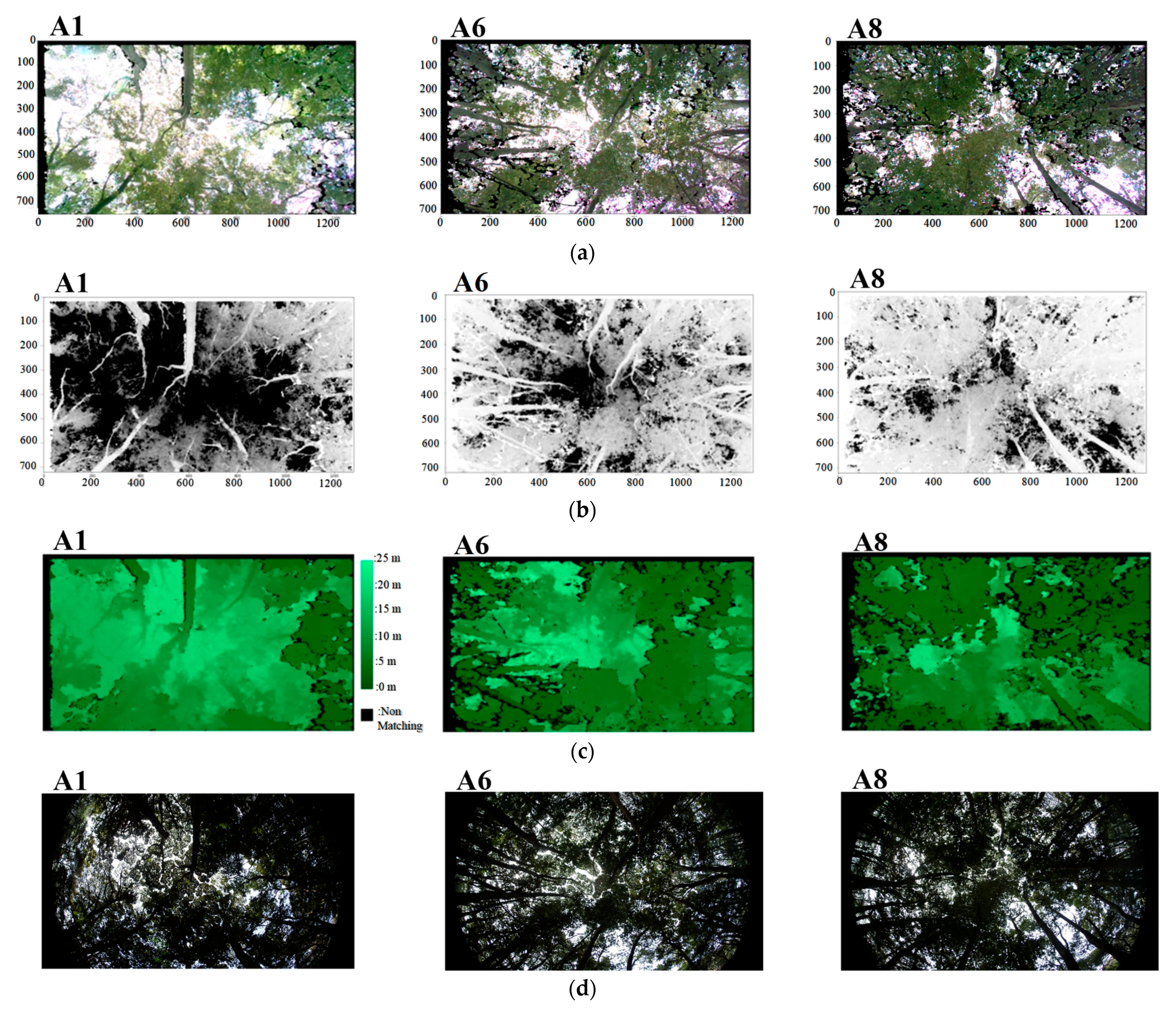
Canopy information based on RGB images, near-infrared, depth images, and fish-eye images during 3 monitoring days differed among nine locations within the plot (Figure 2;

Table 1. Summary of the estimation of canopy openness and total transmittance using Gap Light Analyzer (GLA).

	30 March 2022		21 April 2022		27 April 2022
Location	Canopy Openness (%)	Transmitted Total (%)	Canopy Openness (%)	Transmitted Total (%)	Canopy Openness (%)	Transmitted Total (%)
A1	13.00	12.96	13.02	14.25	12.66	13.23
A2	11.76	9.64	13.99	12.30	14.60	13.93
A3	14.43	10.44	15.09	12.26	17.35	13.13
A4	13.63	10.26	15.88	14.73	20.00	16.80
A5	11.05	7.92	12.53	10.36	13.74	9.51
A6	15.00	13.78	12.13	11.16	14.43	11.45
A7	12.89	16.48	11.02	15.41	12.82	16.91
A8	11.68	14.38	12.70	14.69	13.10	13.54
A9	14.34	12.29	16.44	15.04	17.92	16.44
Mean	13.09	12.02	13.64	13.36	15.18	13.88

). Canopy openness ranged from 11.0 to 20.0% (mean of 14.0; standard deviation of 2.1) (Table 1). Canopy openness values of three representative locations at A1, A6, and A8 were 13%, 15%, and 11.68%, respectively (Figure 2a). The canopy at A8 appears the brightest compared to those at A1 and A6 (Figure 2b), indicating higher near-infrared reflectance, which is quantitatively represented by canopy proportions of 61.9% at A1, 79.8% at A6, and 86.1% at A8. Canopy height distribution varied among the three locations (Figure 2c), with A1 exhibiting the highest proportion of tall trees and A8 dominated by shorter vegetation. Specifically, only 39% of the canopy at A1 was below 10 m, compared to 64% at A6 and 79% at A8, indicating that A6 represents an intermediate structure between A1 and A8 (Figure 2c). Light transmissivity based on fish-eye images ranging from 7.9 to 16.9% for all plots with values of 13.0% for A1, 13.8% for A6, and 14.4% for A8 (Figure 2d; Table 1).

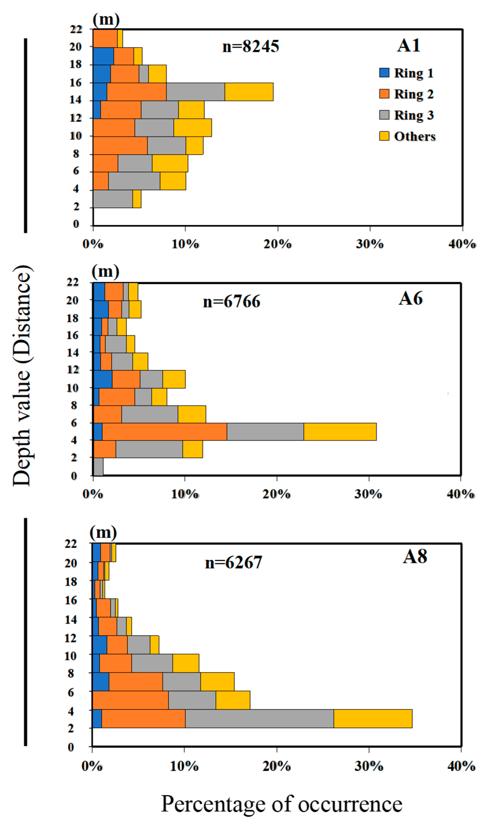
Depth information showed distinct variations in vertical canopy structure among locations within rings (Figure 3). At A1 location, the greatest concentration in rings 2 and 3 mainly occurred within the 14 to 16 m height range, with ring 2 and ring 3 each accounting for 6% (Figure 3). Ring 1 in A6 had a relatively homogeneous distribution of height with 4 to 22 m (Total 10%), while each concentration of ring 2 occurred at 4 to 6 m with 14% (Figure 3). At A8 location, the greatest concentration of rings 2 to 3 occurred in the lowest height with 2 to 4 m with 9% in ring 2 and 16% in ring 3 (Figure 3).

3.2. Estimated LAI and PAI

Both PAI and LAI were obtained separately through image analysis. PAI ranged from 2.23 to 3.68 m² m⁻², with a mean value of 2.97 m² m⁻² and a standard deviation (SD) of 0.38 m² m⁻². LAI ranged from 1.59 to 3.04 m² m⁻², with a mean value of 2.23 m² m⁻² and an SD of 0.29 m² m⁻² (

Table 2. Summary of monitoring and estimation of leaf area index (LAI) and plant area index (PAI).

		Depth Image Sensor							LAI-2200			Fish-Eye Camera
	Location	P	L	L (Upper Canopy)	P (Ring 1)	L (Ring 1)	P (Ring 1 + 2)	L (Ring 1 + 2)	P	P (Ring 1)	P (Ring 1 + 2)	P	P (Ring 1)	P (Ring 1 + 2)
30 March 2022	A1	2.23	1.82	1.24	2.38	2.35	3.86	2.27	3.55	4.49	5.58	3.68	3.57	4.76
	A2	2.86	1.59	0.78	2.37	2.27	3.78	2.64	4.34	3.56	5.46	3.88	3.29	4.30
	A3	2.53	2.09	1.28	3.11	2.41	3.70	2.36	3.93	4.69	5.40	3.44	3.29	4.26
	A4	2.61	2.47	1.13	3.15	3.12	3.55	2.76	3.22	5.18	5.19	3.61	4.68	4.25
	A5	2.94	1.73	0.52	2.66	2.17	3.47	2.19	4.76	5.42	5.16	3.82	4.06	4.19
	A6	3.01	2.40	0.77	2.65	2.51	3.46	2.43	4.56	4.49	5.16	3.48	3.90	4.17
	A7	3.65	2.67	0.48	3.87	3.28	3.45	3.40	4.79	5.77	5.01	3.77	4.84	4.14
	A8	3.31	2.49	0.61	3.80	3.36	3.44	3.19	5.08	5.84	4.95	3.89	4.73	4.11
	A9	2.56	1.88	0.89	2.84	2.57	3.36	2.38	3.74	4.55	4.92	3.52	4.05	4.07
	Mean (SD)	2.85 (0.41)	2.13 (0.37)	0.85 (0.29)	2.98 (0.52)	2.67 (0.43)	3.56 (0.16)	2.62 (0.40)	4.22 (0.60)	4.89 (0.69)	5.20 (0.22)	3.68 (0.16)	4.05 (0.57)	4.25 (0.19)
21 April 2022	A1	2.79	2.29	1.26	2.55	2.52	3.34	2.62	3.93	3.41	4.85	3.64	3.10	4.07
	A2	3.29	2.15	0.75	2.70	2.65	3.20	3.19	4.22	2.92	4.84	3.75	2.82	4.03
	A3	2.65	2.15	1.05	2.98	2.41	3.09	2.27	4.01	3.84	4.79	3.48	3.27	3.99
	A4	2.49	2.28	1.25	2.58	2.56	3.03	2.29	3.76	3.86	4.66	3.27	4.03	3.92
	A5	3.45	2.54	0.42	3.04	3.04	2.92	3.34	4.92	5.03	4.49	3.64	3.95	3.92
	A6	3.68	3.04	0.98	2.82	2.61	2.89	2.82	4.14	2.66	4.46	3.93	3.54	3.88
	A7	3.30	2.22	0.53	3.44	2.75	2.87	2.84	4.57	4.86	4.43	3.92	4.60	3.85
	A8	3.41	2.18	0.59	3.01	2.49	2.86	2.69	5.03	4.77	4.39	3.79	3.86	3.81
	A9	2.93	2.18	0.76	2.76	2.53	2.84	2.39	4.12	3.68	4.35	3.40	3.29	3.79
	Mean (SD)	3.11 (0.38)	2.33 (0.27)	0.84 (0.29)	2.88 (0.26)	2.62 (0.18)	3.00 (0.17)	2.72 (0.36)	4.30 (0.42)	3.89 (0.80)	4.58 (0.19)	3.65 (0.22)	3.60 (0.52)	3.92 (0.09)
27 April 2022	A1	2.82	2.36	1.27	2.52	2.5	2.74	2.61	3.71	3.72	4.16	3.71	3.15	3.78
	A2	3.11	2.05	0.71	2.27	2.23	2.74	2.94	4.14	2.99	4.05	3.91	2.65	3.73
	A3	2.64	2.25	0.99	2.87	2.3	2.69	2.28	4.03	4.06	3.98	3.42	3.11	3.58
	A4	2.48	2.21	1.16	2.56	2.55	2.62	2.30	3.71	3.94	3.94	3.06	3.48	3.57
	A5	3.13	2.05	0.39	2.69	2.01	2.62	2.33	4.92	5.08	3.88	3.67	4.26	3.53
	A6	3.20	2.35	0.65	2.37	2.16	2.61	2.48	4.60	3.71	3.86	3.55	3.25	3.52
	A7	3.13	2.19	0.47	3.46	2.67	2.49	2.82	4.22	4.88	3.84	3.90	4.99	3.44
	A8	3.34	2.39	0.59	3.12	2.59	2.46	2.71	5.00	5.04	3.81	3.75	3.73	3.41
	A9	2.76	2.14	0.88	2.65	2.41	2.46	2.27	3.96	3.69	3.68	3.32	3.39	3.29
	Mean (SD)	2.96 (0.27)	2.22 (0.12)	0.79 (0.29)	2.72 (0.35)	2.38 (0.21)	2.60 (0.11)	2.52 (0.24)	4.25 (0.45)	4.12 (0.68)	3.19 (0.13)	3.59 (0.26)	3.56 (0.66)	3.54 (0.14)
	Total mean (SD)	2.97 (0.38)	2.23 (0.29)	0.83 (0.29)	2.86 (0.41)	2.56 (0.32)	3.06 (0.42)	2.62 (0.35)	4.26 (0.50)	4.30 (0.84)	4.57 (0.56)	3.64 (0.22)	3.74 (0.62)	3.90 (0.33)

Note: L indicates leaf area index (excluding stems and branches). P indicates plant area index. SD indicates standard deviation.

). For each measurement day, mean PAI and LAI on March 30 was 2.85 m² m⁻² (SD: 0.41 m² m⁻²) and 2.13 m² m⁻² (SD: 0.37 m² m⁻²), while mean PAI and LAI was 3.11 m² m⁻² (SD: 0.38 m² m⁻²) and 2.33 m² m⁻² (SD: 0.27 m² m⁻²) on April 21, respectively. PAI on April 27 was 2.96 m² m⁻² (SD: 0.27 m² m⁻²) and LAI was 2.22 m² m⁻² (SD: 0.12 m² m⁻²).

The vertical distribution of foliage was evaluated by estimating the leaf area index (LAI) for the upper canopy (height > 10 m) and the entire canopy using depth image sensor data. The upper canopy LAI was consistently smaller than the total LAI across nine locations, ranging from 0.39 to 1.28 m² m⁻² (17%–68% of total LAI), with a mean of 0.83 m² m⁻² and a standard deviation (SD) of 0.29 m² m⁻² (Table 2). The mean upper canopy LAI values on March 30, April 21, and April 27 were 0.85 m² m⁻² (SD: 0.29 m² m⁻²), 0.84 m² m⁻² (SD: 0.29 m² m⁻²), and 0.79 m² m⁻² (SD: 0.29 m² m⁻²), respectively.

Focusing on the angular distribution, the plant area index (PAI) and LAI for ring 1, as estimated by the depth image sensor, ranged from 2.27 to 3.87 m² m⁻² (mean: 2.86 m² m⁻²; SD: 0.41 m² m⁻²) and 2.01 to 3.36 m² m⁻² (mean: 2.56 m² m⁻²; SD: 0.32 m² m⁻²), respectively (Table 2). For rings 1+2, the PAI and LAI means were 3.06 m² m⁻² (range: 2.46–3.86 m² m⁻²; SD: 0.42 m² m⁻²) and 2.62 m² m⁻² (range: 2.19–3.40 m² m⁻²; SD: 0.35 m² m⁻²), respectively. The proportion of LAI to PAI in ring 1 was 90% on 30 March, 91% on 21 April, and 88% on 27 April, while for rings 1 + 2, it was 74%, 91%, and 97% on the same dates.

Comparisons among devices showed that PAI, estimated using the LAI-2200 and fish-eye images, tended to be greater than those from the depth image sensor. The LAI-2200 PAI values ranged from 3.22 to 5.08 m² m⁻² for all data, 2.66 to 5.84 m² m⁻² for ring 1, and 3.68 to 5.58 m² m⁻² for rings 1 + 2. Fish-eye-derived PAI ranged from 3.06 to 3.93 m² m⁻² for all, 2.65 to 4.99 m² m⁻² for ring 1, and 3.29 to 4.76 m² m⁻² for rings 1 + 2 (Figure 4).

Regression analyses revealed that the depth image sensor exhibited a stronger correlation with the LAI-2200 (R² = 0.58; regression coefficient = 0.58; p < 0.01) compared to the fish-eye images (R² = 0.20; regression coefficient = 0.20; p < 0.05) for total PAI (Figure 4a). For ring 1, fish-eye images showed a higher correlation with the LAI-2200 (R² = 0.65; regression coefficient = 0.60; p < 0.01) than the depth image sensor (R² = 0.48; regression coefficient = 0.34; p < 0.01) (Figure 4b). In contrast, for rings 1 + 2, both methods correlated strongly with the LAI-2200, with R² values of 0.94 for fish-eye images and 0.98 for the depth image sensor (Figure 4c).

3.3. Classification of Canopy Structures

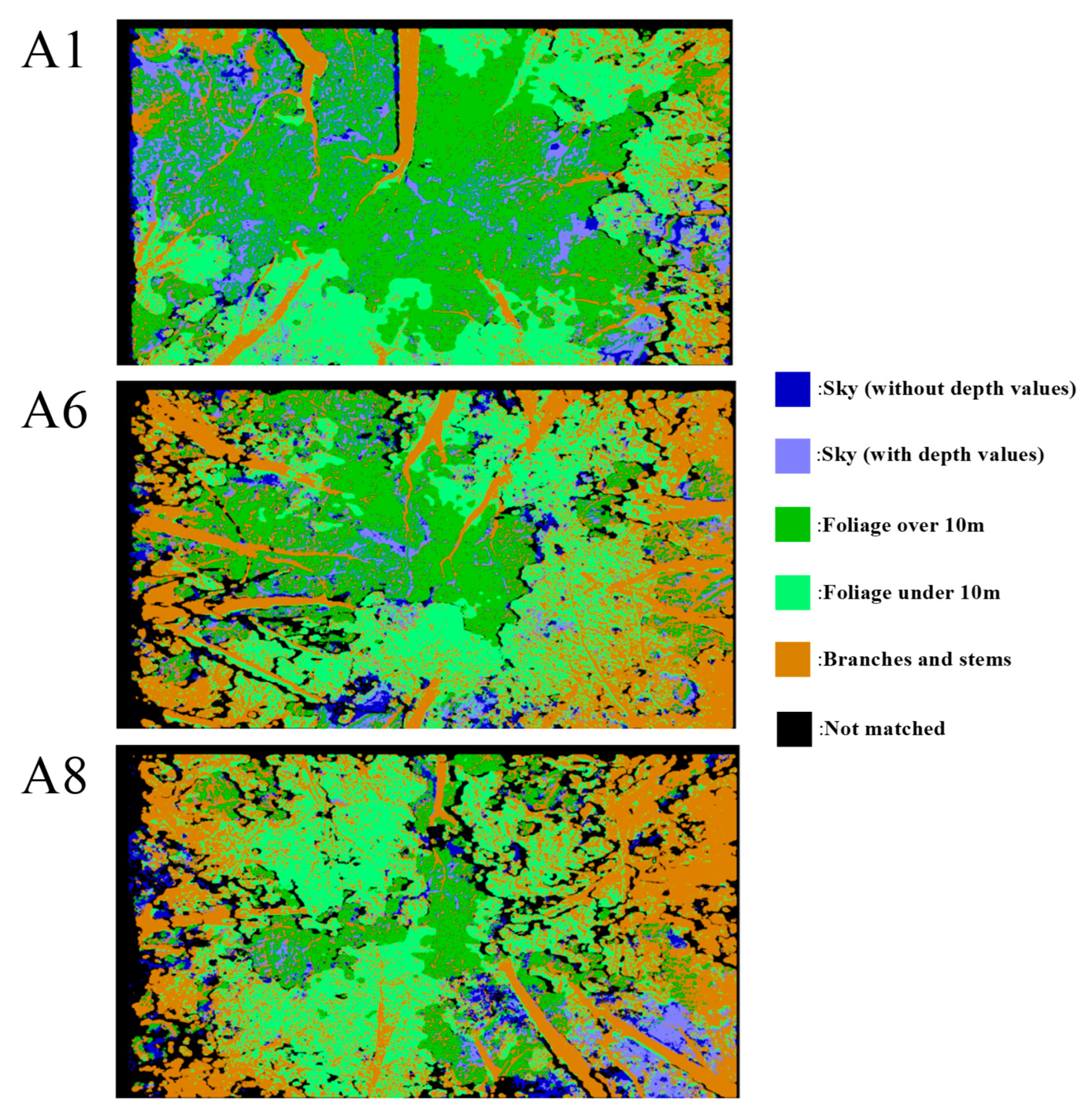
The classification of canopy structures showed the distinctive distribution of foliage above 10 m, foliage below 10 m, and non-assimilating parts (Figure 5 and Figure 6,

Table 3. Summary of the proportions of upper and lower foliage and non-assimilating parts at each measurement point.

	Location	Foliage Over 10 m (%)	Foliage Below 10 m (%)	Branch and Stem (%)
30 March 2022	A1	48%	29%	24%
	A2	26%	41%	32%
	A3	42%	29%	30%
	A4	38%	12%	50%
	A5	12%	55%	33%
	A6	22%	31%	48%
	A7	11%	31%	58%
	A8	12%	36%	52%
	A9	31%	31%	38%
21 April 2022	A1	38%	32%	30%
	A2	21%	31%	48%
	A3	36%	25%	39%
	A4	46%	15%	39%
	A5	9%	35%	56%
	A6	20%	44%	37%
	A7	13%	38%	49%
	A8	13%	44%	43%
	A9	25%	26%	48%
27 April 2022	A1	38%	33%	29%
	A2	21%	32%	47%
	A3	33%	21%	45%
	A4	45%	13%	42%
	A5	10%	40%	51%
	A6	18%	36%	47%
	A7	11%	38%	50%
	A8	12%	41%	47%
	A9	30%	28%	43%

Note: Values rounded; totals may not equal to 100% due to rounding.

). Excluding the sky and non-matching parts for all locations on the three dates, foliage above 10 m ranged from 9 to 48% with 25% of mean values (SD: 0.12), while foliage below 10 m ranged from 12 to 55% with a mean of 32% (SD: 0.10). Non-assimilating parts of all locations on the three dates ranged from 24 to 58%, with 43% of mean values and 0.09 standard deviation (Table 3). At the location of A1, the foliage above 10 m was distributed as major part of the canopy, which consisted of six to seven trunks (non-assimilating parts). Excluding the sky and unclassified parts, the average values across the three dates show that foliage above 10 m in A1 comprised 41% of the total plant leaf area, while foliage below 10 m was 31%, and non-assimilating parts accounted for 28% (Table 3; Figure 5). In A6 and A8, foliage below 10 m was 37 and 40%, with non-assimilating parts being 44% and 47%, respectively (Table 3; Figure 5).

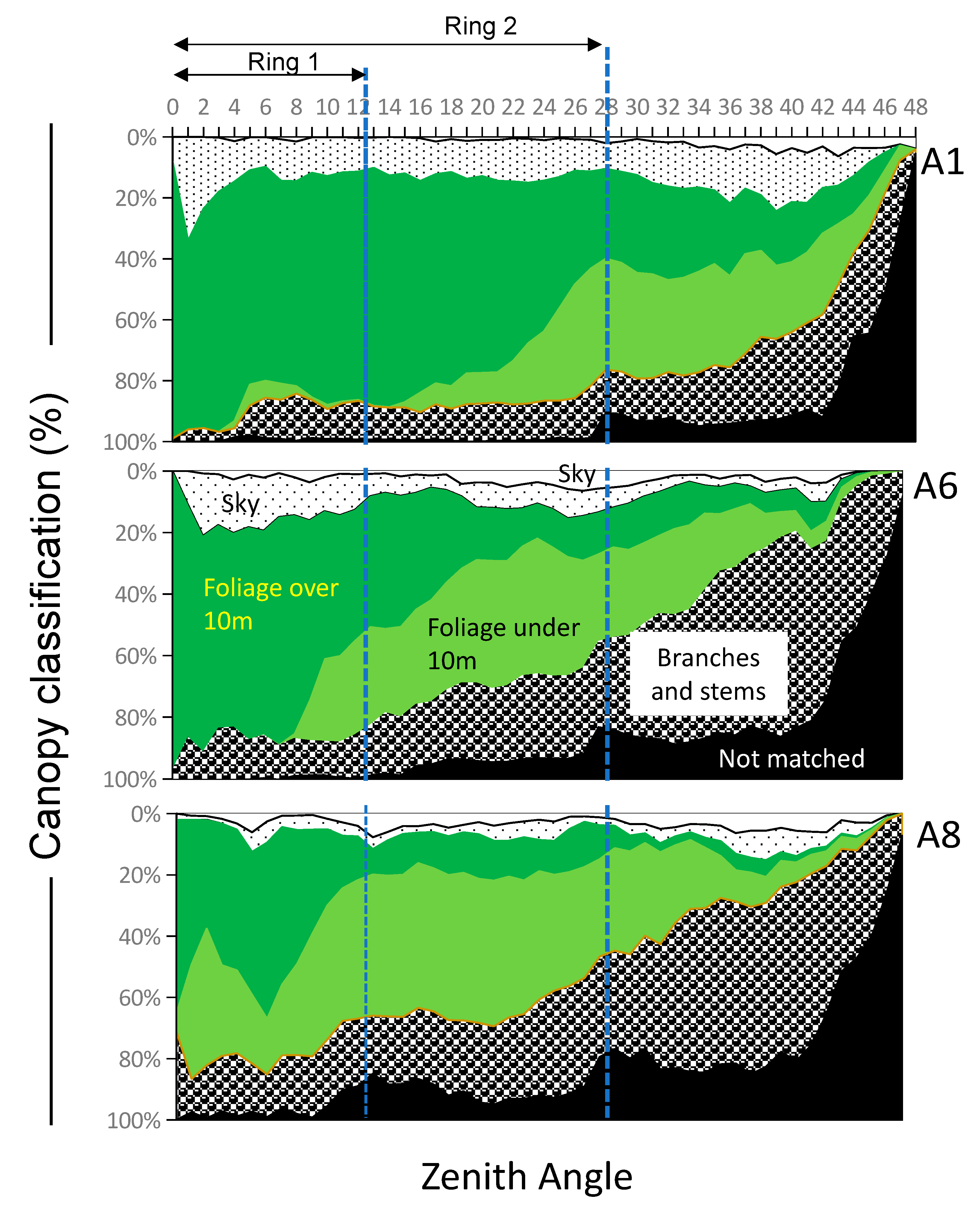
Our classification showed the proportion of coverage rates at different zenith angles (Figure 6). As the zenith angle increases from 0 to 48 degrees, the foliage coverage rate decreases and non-assimilating parts increases, while the patterns differ depending on the canopy structures. For A1, foliage < 10 m increased approximately 25 degrees, and the non-assimilating part started increasing at 35 degrees (Figure 6). For A6 and A8, foliage with >10 m increased from 10 to 15 degrees, while branches and stems increased gradually for the entire zenith angle.

4. Discussion

Our PAI values measured by the depth image sensor, ranging from 2.23 to 3.68 m² m⁻² (mean: 2.97 m² m⁻²; SD:0.38 m² m⁻²), were consistent with previously reported PAI and LAI values. The mean PAI in the evergreen broad-leaved forest dominated by Ubame oak (Quercus phillyraeoides), ring-cupped oak (Quercus glauca), Japanese chinquapin (Castanopsis cuspidata), camphor laurel (Cinnamomum camphora), Japanese bay tree (Machilus thunbergii), and Japanese privet (Ligustrum japonicum) species in Japan has been reported to range from 2.39 ± 0.08 to 3.00 ± 0.28 m² m⁻² across 12 plots, as estimated using the digital photography method [47]. The maximum LAI of the evergreen broad-leaved forest on the eastern slope of Gongga Mountain in the Tibetan Alpine Vegetation Transect (TAVT) region was estimated using the specific leaf area (SLA) biomass conversion method, obtaining a value of 4.17 m² m⁻² [48]. The average PAI of evergreen broad-leaved forests across the entire state of California, USA, was estimated to be 2.94 ± 1.58 m² m⁻² based on GLAS LiDAR data [49]. These comparisons suggest that our depth image sensor-based estimates are within the expected range to the reported PAI and LAI of temperate and subtropical evergreen broad-leaved forests, confirming the sensor’s capability in canopy structural assessment.

This study validated the effectiveness of the LAI estimation method by combining canopy classification to separate leaf area from woody components (e.g., branches and stems). By estimating LAI solely from pixels classified as foliage, the overestimation commonly introduced by non-assimilative parts was minimized. Our results show that PAI was 33%–34% higher than LAI, consistent with previous findings reporting a 27% difference between effective PAI and LAI using terrestrial laser scanning in a temperate broadleaf forest in Oxford, UK (i.e., sycamore, Acer pseudoplatanus; ash, Fraxinus excelsior; hazel, Corylus avellana) [50]. LAI overestimation of 3.0%–31.9% using terrestrial laser scanning in various temperate deciduous broadleaf forests (Fagus sylvatica), temperate Norway spruce forests (Picea abies), and temperate mixed forests in the Bavarian Forest National Park, Germany, has also been reported [51]. These consistencies reinforce the validity of the depth image sensor approach for differentiating structural canopy elements.

In comparing three measurement techniques—depth imaging, LAI-2200, and fish-eye photography—our results show PAI values of 2.23–3.68 m² m⁻², 3.22–5.08 m² m⁻², and 3.06–3.93 m² m⁻², respectively. While standard errors were within 1.4 LAI units, the differences reflect methodological sensitivity. For example, the LAI-2200 may overestimate LAI due to its broader field of view and sensitivity to diffuse light being partially blocked by woody components [52]. Fish-eye photography accuracy has been shown to vary with field of view settings and light conditions [50]. Moreover, although all three methods are based on the gap fraction method, differences in the criteria for determining relative illuminance have led to variations in measurement results. Both the depth image sensor and the LAI-2200 calculate gap fraction using relative illuminance, defined as the ratio of illuminance inside and outside the forest. The LAI-2200 obtains outside-forest illuminance through direct field measurements, whereas the depth image sensor estimates it from the average brightness of the sky seen through canopy gaps inside the forest, significantly improving the convenience and stability of outside-forest illuminance measurement. The fish-eye camera calculates gap fraction by binarizing fish-eye photo into sky and canopy components, without distinguishing between bright and dark sky pixels.

Differences in LAI values across measurement methods also highlight the need to critically assess methodological biases and contextual applicability. Supporting the findings, variation in LAI estimates across the LAI-2000, hemispherical photography, and point-quadrat methods in an Australian evergreen forest, with notable method-specific biases, has been demonstrated [53]. Similarly, a significant divergence in LAI estimates from litter-fall versus direct and optical methods in a Chinese evergreen forest has been reported, attributing differences to methodological limitations such as litter decomposition and light interception errors [54]. These results emphasize the importance of evaluating the assumptions and limitations of each method when selecting an appropriate LAI measurement technique.

Tree size plays a key role in vertical canopy stratification, and our findings demonstrate that depth image sensors effectively capture this structural complexity in Castanopsis sieboldii forests. For instance, in one plot, a large tree (DBH = 50.6 cm) formed the upper canopy, while a smaller individual (DBH = 18.2 cm) occupied the lower layer. These observations are consistent with LiDAR-based studies in the Castanopsis orthacantha and Castanopsis delavayi communities of the Jizu Mountain area in Yunnan [55] and in Okinawa (dominated by Castanopsis sieboldii and Daphniphyllum glaucescens) [56], both of which demonstrated strong relationships between tree diameter and canopy height. The agreement with previous work further supports the utility of the depth image sensor for stratified canopy assessment in complex forest structures. By improving the accuracy of LAI estimation and canopy stratification, this study provides essential data infrastructure for adaptive land and forest management. Accurate spatial characterization of canopy structure enables more informed decisions regarding stand structure optimization, carbon stock assessment, and ecological restoration planning. The reliability of LAI products is critical for climate and ecosystem modeling, especially across diverse land cover types and temporal scales [57]. Moreover, when combined with high-resolution canopy structure maps derived from satellite and airborne observations [58], the field-based sensing approach proposed in this study significantly enhances the capacity to monitor forest structural diversity, which is closely linked to ecosystem resilience and adaptive management potential. In this context, the stratified and spatially explicit canopy metrics developed in this study contribute directly to evidence-based adaptive management strategies in complex forested landscapes.

5. Conclusions

This study addressed two key objectives and demonstrated the potential of depth image sensing for forest canopy characterization. First, the ground-based depth image sensor effectively estimated canopy structure and distinguished non-assimilating components (branches and stems) from foliage, enabling a more accurate LAI estimation. The observed PAI values (2.23–3.68 m² m⁻²) were consistent with previous studies in evergreen broad-leaved forests, supporting the general applicability of the method. By excluding non-assimilating pixels through canopy classification, the approach reduced the common overestimation associated with traditional optical methods. The observed 33%–34% difference between PAI and LAI quantitatively confirmed the effectiveness of this separation. Furthermore, the sensor captured vertical canopy stratification formed by trees of different diameters, highlighting its capability to characterize structurally complex stands. Second, comparison with conventional methods (LAI-2200 and hemispherical photography) demonstrated strong correlations in PAI estimates, despite differences in absolute values. Standard errors were within 1.4 LAI units, indicating sufficient precision for practical applications. In addition, unlike traditional methods, the depth image sensor enables the estimation of external irradiance through canopy gaps, improving operational flexibility and applicability under varied forest conditions.

Despite the significant advances in estimating canopy structures, several challenges remain. For LAI studies, validation using direct methods such as litter collection could improve the accuracy of estimations [21,59]. In addition, the applicability of the depth image sensor across different forest types and under varying light conditions requires further investigation. Nevertheless, our methods and findings highlight the potential of depth image sensing as a practical and scalable tool for forest structural assessment.

References

1. Lowman, M.D.; Rinker, H.B. Forest Canopies, 2nd ed.; Academic Press: San Diego, CA, USA, 2004. [Google Scholar]
2. Bonan, G.B. Forests and climate change: Forcings, feedbacks, and the climate benefits of forests. Science 2008, 320, 1444–1449. [Google Scholar] [CrossRef]
3. Öquist, G.; Huner, N.P.A. Photosynthesis of overwintering evergreen plants. Annu. Rev. Plant Biol. 2003, 54, 329–355. [Google Scholar] [CrossRef]
4. Reich, P.B.; Walters, M.B.; Kloeppel, B.D.; Ellsworth, D.S. Different photosynthesis-nitrogen relations in deciduous hardwood and evergreen coniferous tree species. Oecologia 1995, 104, 24–30. [Google Scholar] [CrossRef]
5. von Arx, G.; Dobbertin, M.; Rebetez, M. Spatio-temporal effects of forest canopy on understory microclimate in a long-term experiment in Switzerland. Agric. For. Meteorol. 2012, 166–167, 144–155. [Google Scholar] [CrossRef]
6. Davies-Colley, R.J.; Payne, G.W.; van Elswijk, M. Microclimate Gradients across a Forest Edge. N. Z. J. Ecol. 2000, 24, 111–121. [Google Scholar]
7. Chen, J.M.; Black, T.A. Defining leaf area index for non-flat leaves. Plant Cell Environ. 1992, 15, 421–429. [Google Scholar] [CrossRef]
8. Monsi, M.; Saeki, T. On the factor light in plant communities and its importance for matter production. Ann. Bot. 2005, 95, 549–567. [Google Scholar] [CrossRef]
9. Holst, T.; Hauser, S.; Kirchgäßner, A.; Matzarakis, A.; Mayer, H.; Schindler, D. Measuring and modelling plant area index in beech stands. Int. J. Biometeorol. 2004, 48, 192–201. [Google Scholar] [CrossRef]
10. Weiss, M.; Baret, F.; Smith, G.J.; Jonckheere, I.; Coppin, P. Review of methods for in situ leaf area index (LAI) determination: Part II. Estimation of LAI, errors and sampling. Agric. For. Meteorol. 2004, 121, 37–53. [Google Scholar] [CrossRef]
11. Ma, C.; Luo, Y.; Shao, M.; Jia, X. Estimation and testing of linkages between forest structure and rainfall interception characteristics of a Robinia pseudoacacia plantation on China’s Loess Plateau. J. For. Res. 2022, 33, 529–542. [Google Scholar] [CrossRef]
12. Fathizadeh, O.; Hosseini, S.M.; Zimmermann, A.; Keim, R.F.; Darvishi Boloorani, A. Estimating linkages between forest structural variables and rainfall interception parameters in semi-arid deciduous oak forest stands. Sci. Total Environ. 2017, 601–602, 1824–1837. [Google Scholar] [CrossRef]
13. Bréda, N.; Granier, A. Intra- and interannual variations of transpiration, leaf area index and radial growth of a sessile oak stand (Quercus petraea). Ann. For. Sci. 1996, 53, 521–536. [Google Scholar] [CrossRef]
14. Wang, Y.R.; Wang, Y.H.; Yu, P.T.; Xiong, W.; Du, A.P.; Li, Z.H.; Liu, Z.B.; Ren, L.; Xu, L.H.; Zuo, H.J. Simulated responses of evapotranspiration and runoff to changes in the leaf area index of a Larix principis-rupprechtii plantation. Acta Ecol. Sin. 2016, 36, 6928–6938. [Google Scholar]
15. Bonan, G.B. Importance of leaf area index and forest type when estimating photosynthesis in boreal forests. Remote Sens. Environ. 1993, 43, 303–314. [Google Scholar] [CrossRef]
16. Norman, J.M.; Campbell, G.S. Canopy structure. In Plant Physiological Ecology; Pearcy, R.W., Ehleringer, J.R., Mooney, H.A., Rundel, P.W., Eds.; Springer: Dordrecht, The Netherlands, 1989; pp. 301–325. [Google Scholar] [CrossRef]
17. Soudani, K.; Trautmann, J.; Walter, J.M. Comparison of optical methods for estimating canopy openness and leaf area index in broad-leaved forests. Comptes Rendus Biol. 2001, 324, 381–392. [Google Scholar] [CrossRef]
18. Gower, S.T.; Norman, J.M. Rapid estimation of leaf area index in conifer and broad-leaf plantations. Ecology 1991, 72, 1896–1900. [Google Scholar] [CrossRef]
19. Liu, F.; Wang, C.; Wang, X. Sampling protocols of specific leaf area for improving accuracy of the estimation of forest leaf area index. Agric. For. Meteorol. 2021, 298–299, 108286. [Google Scholar] [CrossRef]
20. Chen, J.M.; Govind, A.; Sonnentag, O.; Zhang, Y.; Barr, A.; Amiro, B. Leaf area index measurements at Fluxnet-Canada forest sites. Agric. For. Meteorol. 2006, 140, 257–268. [Google Scholar] [CrossRef]
21. Cutini, A.; Matteucci, G.; Mugnozza, G.S. Estimation of leaf area index with the Li-Cor LAI 2000 in deciduous forests. For. Ecol. Manag. 1998, 105, 55–65. [Google Scholar] [CrossRef]
22. Chen, Y.; Zhang, W.; Hu, R.; Qi, J.; Shao, J.; Li, D.; Wan, P.; Qiao, C.; Shen, A.; Yan, G. Estimation of forest leaf area index using terrestrial laser scanning data and path length distribution model in open-canopy forests. Agric. For. Meteorol. 2018, 263, 323–333. [Google Scholar] [CrossRef]
23. Fang, H.; Baret, F.; Plummer, S.; Schaepman-Strub, G. An overview of global leaf area index (LAI): Methods, products, validation, and applications. Rev. Geophys. 2019, 57, 739–799. [Google Scholar] [CrossRef]
24. Gilardelli, C.; Orlando, F.; Movedi, E.; Confalonieri, R. Quantifying the accuracy of digital hemispherical photography for leaf area index estimates on broad-leaved tree species. Sensors 2018, 18, 1028. [Google Scholar] [CrossRef] [PubMed]
25. Penner, M.; White, J.C.; Woods, M.E. Automated characterization of forest canopy vertical layering for predicting forest inventory attributes by layer using airborne LiDAR data. Forestry 2024, 97, 59–75. [Google Scholar] [CrossRef]
26. Brockerhoff, E.G.; Jactel, H.; Parrotta, J.A.; Quine, C.P.; Sayer, J. Plantation forests and biodiversity: Oxymoron or opportunity? Biodivers. Conserv. 2008, 17, 925–951. [Google Scholar] [CrossRef]
27. Uttarakhand Open University. Forest Ecology (MSCBOT-607); Uttarakhand Open University: Haldwani, India, 2023; Available online: https://uou.ac.in/sites/default/files/slm/MSCBOT-607.pdf (accessed on 5 July 2025).
28. Song, Y.; Ryu, Y. Seasonal changes in vertical canopy structure in a temperate broadleaved forest in Korea. Ecol. Res. 2015, 30, 821–831. [Google Scholar] [CrossRef]
29. Olivas, P.C.; Oberbauer, S.F.; Clark, D.B.; Clark, D.A.; Ryan, M.G.; O’Brien, J.J.; Ordoñez, H. Comparison of direct and indirect methods for assessing leaf area index across a tropical rain forest landscape. Agric. For. Meteorol. 2013, 177, 110–116. [Google Scholar] [CrossRef]
30. Japan Meteorological Agency. Available online: https://www.jma.go.jp/jma/indexe.html (accessed on 8 April 2024).
31. Biodiversity Center of Japan. Available online: https://www.biodic.go.jp/index_e.html (accessed on 12 May 2024).
32. Liu, Z.; Wang, X.; Chen, J.M.; Wang, C.; Jin, G. On improving the accuracy of digital hemispherical photography measurements of seasonal leaf area index variation in deciduous broadleaf forests. Can. J. For. Res. 2015, 45, 721–731. [Google Scholar] [CrossRef]
33. Chianucci, F.; Bajocco, S.; Ferrara, C. Continuous observations of forest canopy structure using low-cost digital camera traps. Agric. For. Meteorol. 2021, 307, 108516. [Google Scholar] [CrossRef]
34. Bater, C.W.; Coops, N.C.; Wulder, M.A.; Hilker, T.; Nielsen, S.E.; McDermid, G.; Stenhouse, G.B. Using digital time-lapse cameras to monitor species-specific understorey and overstorey phenology in support of wildlife habitat assessment. Environ. Monit. Assess. 2011, 180, 1–13. [Google Scholar] [CrossRef]
35. Intel Corporation. Intel RealSense D400 Series Datasheet. Available online: https://www.intelrealsense.com/wp-content/uploads/2022/03/Intel-RealSense-D400-Series-Datasheet-March-2022.pdf (accessed on 18 June 2024).
36. LI-COR Biosciences. LAI-2200C Instruction Manuals. Available online: https://www.licor.com/support/MicroContent/Resources/MicroContent/manuals/lai-2200c-instruction-manuals.html (accessed on 24 June 2024).
37. Danner, M.; Locherer, M.; Hank, T.; Richter, K. Measuring Leaf Area Index (LAI) with the LI-Cor LAI 2200C or LAI-2200 (+2200Clear Kit)—Theory, Measurement, Problems, Interpretation; EnMAP Field Guide Technical Report; GFZ Data Services: Potsdam, Germany, 2015. [Google Scholar] [CrossRef]
38. ter Steege, H. Hemiphot. R: Free R Scripts to Analyse Hemispherical Photographs for Canopy Openness, Leaf Area Index and Photosynthetic Active Radiation Under Forest Canopies; Unpublished Report; Naturalis Biodiversity Center: Leiden, The Netherlands, 2018. [Google Scholar]
39. Frazer, G.W.; Canham, C.D.; Lertzman, K.P. Gap Light Analyzer (GLA), Version 2.0: Imaging Software to Extract Canopy Structure and Gap Light Transmission Indices from True-Colour Fisheye Photographs, User’s Manual and Program Documentation; Simon Fraser University: Burnaby, BC, Canada; Institute of Ecosystem Studies: Millbrook, NY, USA, 1999. [Google Scholar]
40. Intel Corporation. C/C++ Code Samples for Intel RealSense SDK 2.0. Intel® RealSense™ Developer Documentation. Available online: https://dev.intelrealsense.com/docs/code-samples (accessed on 24 July 2024).
41. Maphanga, T. The use of modified and unmodified digital cameras to monitor small-scale savannah rangeland vegetation. J. Rangel. Sci. 2025, 15, 1–8. [Google Scholar] [CrossRef]
42. Kirk, K.; Andersen, H.J.; Thomsen, A.G.; Jørgensen, J.R.; Jørgensen, R.N. Estimation of leaf area index in cereal crops using red–green images. Biosyst. Eng. 2009, 104, 308–317. [Google Scholar] [CrossRef]
43. Zheng, G.; Moskal, L.M. Retrieving leaf area index (LAI) using remote sensing: Theories, methods and sensors. Sensors 2009, 9, 2719–2745. [Google Scholar] [CrossRef] [PubMed]
44. Campbell, G.S.; Norman, J.M. The description and measurement of plant canopy structure. In Plant Canopies: Their Growth, Form and Function; Marshall, B., Russell, G., Jarvis, P.G., Eds.; Cambridge University Press: Cambridge, UK, 1989; pp. 1–20. [Google Scholar] [CrossRef]
45. de Castro, F.; Fetcher, N. Three dimensional model of the interception of light by a canopy. Agric. For. Meteorol. 1998, 90, 215–233. [Google Scholar] [CrossRef]
46. Barclay, H.J.; Trofymow, J.A.; Leach, R.I. Assessing bias from boles in calculating leaf area index in immature Douglas-fir with the LI-COR canopy analyzer. Agric. For. Meteorol. 2000, 100, 255–260. [Google Scholar] [CrossRef]
47. Sasaki, T.; Imanishi, J.; Ioki, K.; Morimoto, Y.; Kitada, K. Estimation of leaf area index and canopy openness in broad-leaved forest using an airborne laser scanner in comparison with high-resolution near-infrared digital photography. Landsc. Ecol. Eng. 2008, 4, 47–55. [Google Scholar] [CrossRef]
48. Luo, T.; Neilson, R.P.; Tian, H.; Vörösmarty, C.J.; Zhu, H.; Liu, S. A model for seasonality and distribution of leaf area index of forests and its application to China. J. Veg. Sci. 2002, 13, 817–830. [Google Scholar] [CrossRef]
49. Tang, H.; Dubayah, R.; Brolly, M.; Ganguly, S.; Zhang, G. Large-Scale Retrieval of Leaf Area Index and Vertical Foliage Profile from the Spaceborne Waveform Lidar (GLAS/ICESat). Remote Sens. Environ. 2014, 154, 8–18. [Google Scholar] [CrossRef]
50. Calders, K.; Origo, N.; Disney, M.; Nightingale, J.; Woodgate, W.; Armston, J.; Lewis, P. Variability and Bias in Active and Passive Ground-Based Measurements of Effective Plant, Wood and Leaf Area Index. Agric. For. Meteorol. 2018, 252, 231–240. [Google Scholar] [CrossRef]
51. Zhu, X.; Skidmore, A.K.; Wang, T.; Liu, J.; Darvishzadeh, R.; Shi, Y.; Premier, J.; Heurich, M. Improving Leaf Area Index (LAI) Estimation by Correcting for Clumping and Woody Effects Using Terrestrial Laser Scanning. Agric. For. Meteorol. 2018, 263, 276–286. [Google Scholar] [CrossRef]
52. Ryu, Y.; Sonnentag, O.; Nilson, T.; Vargas, R.; Kobayashi, H.; Wenk, R.; Baldocchi, D.D. How to Quantify Tree Leaf Area Index in an Open Savanna Ecosystem: A Multi-Instrument and Multi-Model Approach. Agric. For. Meteorol. 2010, 150, 63–76. [Google Scholar] [CrossRef]
53. Coops, N.C.; Smith, M.L.; Jacobsen, K.L.; Martin, M.; Ollinger, S. Estimation of Plant and Leaf Area Index Using Three Techniques in a Mature Native Eucalypt Canopy. Austral Ecol. 2004, 29, 332–341. [Google Scholar] [CrossRef]
54. Ren, H.; Peng, S.-L. Comparison of methods for estimating leaf area index in Dinghushan forests. Acta Ecol. Sin. 1997, 17, 220–223. (In Chinese) [Google Scholar]
55. Rao, J.; Yang, T.; Tian, X.; Liu, W.; Wang, X.; Qian, H.; Shen, Z. Vertical Structural Characteristics of a Semi-Humid Evergreen Broad-Leaved Forest and Common Tree Species Based on a Portable Backpack LiDAR. Biodivers. Sci. 2023, 31, 23216. [Google Scholar] [CrossRef]
56. Zawawi, A.A.; Shiba, M.; Jemali, N.J.N. Accuracy of LiDAR-Based Tree Height Estimation and Crown Recognition in a Subtropical Evergreen Broad-Leaved Forest in Okinawa, Japan. For. Syst. 2015, 24, e002. [Google Scholar] [CrossRef]
57. Fotis, A.T.; Morin, T.H.; Fahey, R.T.; Hardiman, B.S.; Bohrer, G.; Curtis, P.S. Forest structure in space and time: Biotic and abiotic determinants of canopy complexity and their effects on net primary productivity. Agric. For. Meteorol. 2018, 250, 181–191. [Google Scholar] [CrossRef]
58. de Conto, T.; Armston, J.; Dubayah, R. Characterizing the structural complexity of the Earth’s forests with spaceborne lidar. Nat. Commun. 2024, 15, 8116. [Google Scholar] [CrossRef] [PubMed]
59. Dufrêne, E.; Bréda, N. Estimation of deciduous forest leaf area index using direct and indirect methods. Oecologia 1995, 104, 156–162. [Google Scholar] [CrossRef]
Figure 1. Location and overview of the study site: (a) location of the study site, indicated by a red star; (b) overview of the study site taken on 30 March 2022; (c) depth image sensor measurement taken on 30 March 2022; (d) canopy projection and measurement locations.
Forests 16 01294 g001
Figure 2. Five-band depth images and corresponding fish-eye images at locations A1, A6, and A8, which represent different measurement locations: (a) visible red, green, blue (RGB) image; (b) near-infrared image; (c) depth image; (d) fish-eye image.
Forests 16 01294 g002
Figure 3. Distribution of canopy depth values at different heights at locations A1, A6, and A8. Others represent unrecognized parts.
Forests 16 01294 g003
Figure 4. Comparison of plant area index (PAI) estimated by depth image sensor and fish-eye photography with respect to LAI-2200 measurements: (a) PAI from total images; (b) PAI from ring 1; (c) PAI from ring 1 + 2. The blue and yellow dashed lines represent linear regression lines for the depth image sensor and fish-eye photo estimates, respectively.
Forests 16 01294 g004
Figure 5. Classification of canopy structure at locations A1, A6, and A8 (measured on 30 March 2022).
Forests 16 01294 g005
Figure 6. Canopy classification at locations A1, A6, and A8 across different zenith angle ranges (measured on 30 March 2022). The colors represent canopy components: white for sky, dark green for foliage above 10 m, light green for foliage below 10 m, hatched for branches and stems, and black for unmatched areas.
Forests 16 01294 g006