Abstract
Forests play a crucial role in storing excess carbon released into the atmosphere. By mitigating climate change, forest carbon stocks play a vital role in achieving green transitions. However, limited information is available regarding the factors that affect forest carbon stocks. The primary objective of this analysis is to investigate the impact of green agricultural technologies and bioenergy on forest carbon stocks. The empirical investigation was conducted using the method of moments quantile regression (MMQR) technique. Results using the MMQR approach indicate that bioenergy is beneficial in augmenting forest carbon stores at all levels. A 1% increase in bioenergy is associated with an increase in forest carbon stocks ranging from 3.100 at the 10th quantile to 1.599 at the 90th quantile. In the context of developing economies, similar findings are observed; however, in developed economies, bioenergy only fosters forest carbon stocks at lower and middle quantiles. In contrast, green agricultural technologies have an adverse effect on forest carbon stocks. Green agricultural technologies have a significant negative impact on forest carbon stocks, particularly between the 10th and 80th quantiles, with their influence declining in magnitude from −2.398 to −0.619. This negative connection is observed in both developed and developing countries at most quantiles, except for higher quantiles in developed economies. Gross domestic product (GDP) has an adverse effect on forest carbon stores only in developing countries, whereas human capital diminishes forest carbon stocks in both developed and developing nations. Governments should provide support for the creators of bioenergy and agroforestry technologies so that forest carbon stocks can be increased.
1. Introduction
Environmental degradation and its implications for the world have become a significant concern. Emissions of greenhouse gases, particularly carbon dioxide (CO2), are the primary reason behind global climate change and the resulting environmental degradation. Forests have the ability to sequester CO2 emissions and store them in tree biomass, thereby helping to mitigate damage to the ecosystem [1]. Carbon sequestration is the process of capturing and storing atmospheric carbon dioxide [2]. A report by the Intergovernmental Panel on Climate Change (IPCC) [3] stated that deforestation and forest degradation account for approximately 13% of the global carbon footprint. The services of forests to the ecosystem are not limited to the sequestration and absorption of CO2 emissions; their ability to offer a source of clean raw materials is one of the most outstanding services to the ecosystem. However, both these approaches offer contrasting outcomes. On the one hand, wood harvesting diminishes forest carbon stores, thereby impairing its capacity to function as a carbon reservoir [4]. In contrast, a reduction in wood harvesting can enhance the carbon sequestration ability of forests while significantly limiting their capacity to supply wood for energy production and meet societal material demands [5]. Strategies used to combat climate change often emphasize the increased reliance on forests and trees to produce biomass energy rather than fossil fuels. Although forest biomass is generally believed to be carbon-neutral, this viewpoint remains controversial in the scientific community [6]; therefore, the role of forest biomass in the global fight against climate change is a topic that requires more attention.
To achieve bioeconomy objectives in countries with abundant forests, a technology-driven biomass-based bioeconomy can play a crucial role [7]. India, where forests cover almost 21.71% of the country’s land, is a good reference to support our understanding of the ways in which forest biomass and value-added products produced by forests can help materialize the target of reaching USD 300 billion in the bioeconomy by 2030, which requires that we reach USD 100 billion by 2025 [8]. Consequently, augmenting the net primary efficiency of forests to achieve higher biomass output should be regarded as a crucial approach, alongside novel biotechnology, to enhance agricultural output, waste recycling, medical uses, and alternative power sources in order to fulfil societal and ecological objectives. This method would enhance the strategic edge of forest-rich nations in establishing their bioeconomies. The increased forest area, with substantial carbon stock, would strengthen the prospects for a carbon market in these nations, helping to build a clean and green economy [9]. The increased forest area with substantial carbon stock would strengthen prospects for a carbon market in these nations, thus contributing to a green economy. The precise assessment of tree biomass and carbon reserves is essential for the development and execution of a successful bioresource generation and extraction strategy. This calculation provides essential insights into the precise amount and distribution of biomass and carbon sequestered in trees, facilitating informed decisions in resource design and allocation. By precisely quantifying tree biomass and carbon reserves, organizations can optimize their operations while ensuring environmental responsibility and effective logistics to meet their bioeconomy objectives [10].
In addition to the forests, the agriculture sector contributes to the bioeconomy and to global carbon stock. Agriculture’s contribution to greenhouse gas emissions was 22% in 2019 [11]. The agricultural sector’s contribution to global greenhouse gas emissions has remained relatively stable since 2019. This decline can be attributed to an increased reliance on green agricultural technologies, as the use of such technologies enables an optimized and creative distribution of production components, which may lead to a decrease in agricultural-related CO2 emissions and ultimately foster sustainable agricultural growth. This serves as a primary motivation for investigating the effects of pathways on the advancement of green technologies aiming to reduce agricultural carbon emissions, which account for almost 20% of global emissions and ultimately impact the overall carbon stock of forests. The development of green technology is a multifaceted phenomenon influenced by numerous internal and external factors. Green agricultural technologies primarily belong to two separate categories. The first category includes resource-conservation green technology, while the second category includes green technology that helps control carbon emissions [12]. Both work simultaneously to mitigate the impact of climate change by conserving resources, improving efficiency, and reducing CO2 emissions. The global carbon stocks in forests decreased slightly between 1996 and 2022. Meanwhile, emerging and developing economies have a larger share of carbon stocks in forests compared to advanced economies.
CO2 emissions are widely considered to be the single largest contributor to global climate change; a large amount of empirical evidence has been used to estimate the factors that can influence global carbon footprints, such as information and communications technology (ICT) [13], globalization [14], renewable energy [15], urbanization [16], and financial development [17], among others. While the available literature has examined the factors affecting forest carbon stocks, comprehensive and cross-country analyses that can be used to estimate the influence of technological, energy, social, and economic factors on forest carbon stocks are lacking. Particularly, the literature has not specifically examined the impact of green agricultural technologies and bioenergy on forest carbon stock.
Thus, a noticeable gap exists in the literature. This analysis tries to fill the aforementioned gap in the literature by estimating the influence of agricultural technologies and bioenergy on forest carbon stocks. Therefore, the analysis makes the following contribution by adding several novel points to the literature. The first novelty of the analysis is examining the influence of green agricultural technologies on forest carbon stocks in top bioenergy-producing economies. Moreover, the top bioenergy-producing economies include both developed and developing economies that are investing heavily in the technological domain, as well as the top carbon emitters in the world. Analysing the connection between green agricultural technologies and forest carbon stocks in these economies is vital in enhancing our understanding of how green technological development within the agricultural sector can impact global carbon forest stocks. The second novel addition to the study aims to shed light on the connection between bioenergy and forest carbon stock in the 26 top bioenergy-producing economies. This provides insight into how leading bioenergy-producing countries influence forest carbon stocks. A third important contribution of the analysis is the application of the MMQR technique, which provides robust estimates and facilitates the examination of the asymmetric influence of green agricultural technologies and bioenergy on forest carbon stocks. Lastly, the study’s outcomes provide practical suggestions to concerned stakeholders on enhancing the forest’s ability to absorb CO2 emissions while offering valuable and sustainable raw materials for the development of a bioeconomy.
2. Theoretical Framework
Green growth in agriculture has emerged as a crucial concept, garnering significant worldwide interest. To achieve sustainable growth in green agriculture and address the critical challenges of agricultural resource scarcity and ecological deterioration, green agricultural technologies have become a fundamental approach. Green agricultural technologies are crucial in reducing chemical use, improving soil condition, and ultimately lowering environmental pollution [18]. In contrast, green agricultural technologies can sometimes prove detrimental to the ecosystem due to their positive role in enhancing agricultural activities. Increased agricultural activities require more land, and farmers fulfil this requirement by clearing forest land, leading to enhanced deforestation, reduced biodiversity, and harm to natural ecosystems [19]. Green technology includes techniques and tools that help reduce the overuse of natural resources by making production and consumption more efficient. Thus, green technology plays a crucial role in protecting the ecosystem by reducing pollutants, conserving energy, and promoting eco-friendly alternatives [20]. Technological innovation enhances energy efficiency by conserving inexpensive manufacturing resources and reducing energy consumption per unit of output, thereby contributing to a decrease in CO2 emission levels. While technological progress is not inherently neutral, understanding the advantages of certain production variables and individuals in the economy necessitates that we recognise that such advancements would reduce CO2 emission concentrations via various mechanisms [21]. Green agricultural technologies, such as precision farming, improved seeds, organic fertilizers, and efficient irrigation systems, increase per-acre yield and enhance overall agricultural output without requiring additional land [22]. Then, there is no need to use extra farmland, so forests will be protected, resulting in a greater availability of forests for storing carbon.
On the other hand, large-scale and combined farming may require a significant portion of land, thereby encouraging deforestation and reducing the forest’s ability to store carbon. Thus, the relationship between green agricultural technologies and forest carbon stock depends on whether these technologies and methods lead to an increase in the use of forest land for agricultural practices [23].
Biomass energy has become a crucial component in global discussions on energy policy and sustainability efforts because it is an essential part of clean and green energy sources [24]. In 2019, approximately 2.6 billion people—one-third of the global population—utilised traditional fuels such as wood, charcoal, and crop residues for cooking. In low- and middle-income countries, biomass and charcoal made up about 88% of these fuels [25]. Biomass energy has several applications in the production of chemicals, as a fuel for logistics and transportation, and in heating and electricity generation. This form of energy has been used for many centuries, and in the past, it was mostly used for cooking and heating. Since it is abundant, plentiful, and low in carbon, it is regarded as the best possible substitute for fossil fuels. Due to the growing demand for bioenergy, the production of biofuels, such as ethanol and biodiesel, which utilize crops (e.g., maize, sugarcane), has contributed to the global expansion of agriculture [26]. Nevertheless, these operations have negative economic and ecological consequences, including increased volatility in food prices and the utilization of more land for agriculture that is not suitable for cultivation. Particularly, agricultural rivalry between the food and energy industries might cause food prices to fluctuate more. Furthermore, the conversion of additional agricultural areas from forests, destroyed forests, or grasslands has detrimental effects on the ecosystem [27]. Since forests are used to absorb or sequester carbon, the increased use of agricultural land for biofuel production may lead to increased CO2 emissions into the ecosystem [28]. Thus, bioenergy can either positively or negatively influence forest carbon stock.
3. Econometric Model
The primary objective of this analysis is to examine the impact of green agricultural technologies, bioenergy, GDP, financial development, and human capital on forest carbon stocks. Carbon sequestration is one of the main features of forests, and it is influenced by several factors. To construct an empirical model of carbon stock function, the present study used the models developed by Soto et al. [29] and Meeussen et al. [30]. The model has been augmented by incorporating relevant variables, resulting in the following functional form of forest carbon stock:
where forest carbon stock is determined by bioenergy (BE), green agricultural technologies (GAT), gross domestic product (GDP), financial development (FD), and human capital (HC). is the constant, indicates the coefficients, and ε is the error term. Green agricultural technologies are expected to positively (+) influence forest carbon stock. The increased reliance on green forest technologies within the agricultural sector can significantly increase output levels while using the same amount of land. In other words, the per-acre yield surges significantly due to the increased adoption of green technologies. Consequently, the agricultural sector does not require more land for cultivation; thereby, the forest land is protected, as well as its carbon-storing ability. Bioenergy can either positively or negatively (+/−) influence forest carbon stocks. The burning of wood is one of the largest sources of bioenergy, which can accelerate the pace of deforestation and reduce its ability to store carbon. On the other hand, bioenergy produced through more sustainable methods can reduce the strain on forest resources, thereby reducing deforestation and tree cutting, and thus enhancing forest carbon stocks. GDP can also impact the forest carbon stock in both ways, i.e., positively (+) or negatively (−). The negative effect arises in the initial phases of economic growth, where urbanisation, industrialisation, and large-scale development consume large areas of forest land, negatively impacting forest carbon stocks. In contrast, the positive effect emerges at a high level of economic development, where nations begin to focus on a cleaner and greener environment and implement stringent policies to curb environmental pollution and preserve natural resources, including forests. Financial development can have both positive (+) and negative (−) influences on forest carbon stocks. Financial development can positively influence forest carbon stocks by providing financial support for the development of clean energy technologies and green ventures at affordable rates, which are crucial for the preservation of forests and other natural resources. In contrast, financial development can catalyse economic activity, which significantly enhances environmental pollution and damages forest resources, thereby reducing the ability of forests to sequester carbon. Human capital is expected to have a positive impact on the forest carbon stock. A more educated and skilled workforce behaves more responsibly in protecting the ecosystem and forest resources, thereby increasing the ability of forests to absorb carbon.
4. Econometric Methodology
4.1. CSD and Homogeneity Tests
The issue of cross-sectional dependence (CSD), as discussed by De Hoyos and Sarafidis [31], serves as a foundational aspect of the panel data paradigm. The issue of CSD concerning geographical connections, transmission effects, and common unobserved disruptions must be resolved. Ignoring the CSD issue results in inaccurate calculations and conclusions being made. Consequently, several tests, such as the Friedman test, the Breusch and Pagan test, the Frees test, and the Pesaran test, have been introduced to address this issue [32,33]. In this analysis, the study relies on the Pesaran [34] CSD test to check the existence of cross-sectional dependency. The following is the generic equation representing this test:
In the above equation, T represents the periods, N represents the cross-sections, while represents the pair-wise association of residuals between cross-sectional units i and k = i + 1. Slope heterogeneity is crucial in panel analysis because of the impact of regressors (bioenergy, green agricultural technologies, GDP, financial development, and human capital). Ignoring this problem will lead to unreliable and biased estimations being made. To address this, slope heterogeneity within nations was investigated using the Pesaran and Yamagata heterogeneity test [35].
where N represents the number of nations, S signifies the Swamy test statistic, and K symbolises the regressors. The delta statistic and its mean-variance-biased adjusted delta counterpart presuppose that the error terms must exhibit homoscedasticity and no autocorrelation.
4.2. Panel Unit Root Tests and Co-Integration Tests
The third essential step in panel analysis is examining the panel unit roots properties. The available empirical works on energy and environment proposed two techniques for unit root testing. The alternative hypothesis is tested against the null hypothesis, which states that all variables have a unit root. First-generation unit root tests were developed by Maddala and Wu [36], Choi [37], and Bai and Ng [38]. These tests do not address the CSD issue and thereby lead to erroneous conclusions. The necessity to overcome the CSD assumption, however, led to the development of second-generation unit root tests, including the cross-sectional augmented Dickey–Fuller (CADF) and cross-sectional augmented Im–Pesaran–Shin (CIPS) tests; these are capable of overcoming the issues of CSD and thereby they help us to detect the true nature of the integration properties of the available variables [39]. The CADF is based on the following generic equation:
where the cross-sectional average is signified by helps in estimating the ADF. The above specification (5) facilitates the derivation of the CIPS equation by employing the mean individual (CADF) approach across the N cross-sections and T time periods.
In the previous step, after verifying the stationarity properties, it is essential to confirm whether a long-term relationship exists between FCS, GAT, BE, FD, GDP, and HC. To achieve this, the study employs the panel Pedroni co-integration test [40]. This test has the ability to handle non-stationary data and account for heterogeneity across different cross-sections.
4.3. MMQR Method
Conventional econometric techniques have been employed in most past energy and environment studies. However, the traditional approaches rely on the normalcy criterion for assessing the relationship between the selected variables. The outcomes derived from these methods are not optimal for examining the relationship between variables at precise locations within the joint distribution. To counter the issue of normalcy, the quantile regression approach, as specified by Koenker and Bassett [41], is an optimal approach. Recent studies have prominently emphasised the integration of quantile-based estimation methods with panel data [42,43]. To identify variation between cross-sections, fixed-effects models are used in a conventional panel data framework. A similar quantile regression approach, incorporating a fixed effect, is also available and has been used in several studies. Prior efforts that rely on fixed effects using quantile regression have focused on the challenges of estimating fixed effects within a quantile framework and the parameter complications when T is minimal. Machado and Silva [44] developed a novel quantile regression approach for panel data to address this issue. The primary advantage of Machado and Silva [44] regression compared to existing quantile methods is in the incorporation of additive fixed effects. Furthermore, it is a suitable approach for countering data with non-normal distributions, as it allows for the use of techniques specifically designed for estimating conditional means, while demonstrating the influence of the independent variable on the total conditional distribution. Another prominent feature of the MMQR that distinguishes it from other quantile-based approaches is its ability to control for regressors that exhibit endogeneity [45]. The MMQR produces results using regression quantiles that are not overlapping, a crucial criterion that is sometimes overlooked in empirical settings [44]. Consequently, the MMQR approach is adopted. The conditional quantiles estimate that signifies the location-scale variant model is expressed in Equation (7), given below:
where country-specific fixed effects are signified by , the number of years is signified by t = 1, …, t, and L is the K-vector having unknown regressors. Using this information, Equation (3) can be respecified in the following final form proposed by Machado and Silva [44]:
where and signify the quantile distribution of the outcome variables and the vector of regressors, correspondingly. Lit − ϕ(τ) ≡ ϕi + λiq(τ) signifies the scalar coefficient indicating the fixed-effect quantile, τ, for the corresponding cross-section, i.
4.4. Robustness Estimation Methodologies
Apart from MMQR, some additional approaches, such as fully modified ordinary least square (FMOLS) of Phillips and Hansen [46] and Chudik and Pesaran [47], are also applied to test the robustness of our primary estimates. The FMOLS is a non-parametric approach specifically designed to examine the co-integration relationship between variables while controlling for the issues of endogeneity and correlation that may exist due to cross-section variables. Dynamic common correlated effect (DCCE) is an error-correction-based approach that addresses three primary issues: the CSD, heterogeneity, and endogeneity [48]. For both long- and short-term results, the study employed the cross-sectional augmented autoregressive distributed lag (CS-ARDL) and pooled mean group autoregressive distributed lag (PMG-ARDL) methods. The CS-ARDL method is more reliable in addressing CSD and endogeneity problems [49]. The PMG-ARDL model, which belongs to the ARDL family, can also be utilized. The distinct feature of this method is its ability to address the endogeneity issue [50]. Many recent studies in energy and environmental economics use this method for panel data analysis.
5. Data and Summary Statistics
This paper assesses the impact of green agricultural technologies and bioenergy on forest carbon stocks by utilising panel data from the top 26 bioenergy-producing countries from 1996 to 2022. This timeframe is chosen primarily based on the continuous availability of data across all concerned variables included in the study. The list of sample countries is reported in Table A1 of Appendix A. The dependent variable, forest carbon stocks (FCS), is primarily measured in terms of carbon stocks in forests, expressed in million tonnes. The data on forest carbon stocks is obtained from the International Monetary Fund (IMF). Means stocks of forest carbon are presented for sample economies in Figure 1. The independent variables in our research are bioenergy (BE) and green agricultural technologies (GATs). Consistent with the study by Sohail et al. [51], biofuels production in quad Btu is used to measure bioenergy. Bioenergy is derived from forest sources, indicating that it has both direct and indirect implications for forest carbon dynamics. The number of total patents in adaptation technologies for agriculture, forestry, livestock production can be looked to as a reflection of the number of green agricultural technologies; following the previous literature [52], the number of patents related to green agricultural technologies is used as a proxy measure for the number of green agricultural technologies. The data on bioenergy are obtained from the EIA, and the data on green agricultural technology are collected from the Organisation for Economic Cooperation and Development (OECD). The control variables include gross domestic product (GDP), financial development (FD), and human capital (HC). The selection of these control variables is based on prior research. Studies document significant effects of these control variables on forest carbon stock. The literature discusses both the positive and negative effects of GDP on forest carbon stocks. According to Ewers [53], an upsurge in GDP initially leads to increased deforestation due to infrastructure development, agricultural expansion, and logging activities. As countries reach higher income thresholds, increased investment in sustainable land use, the adoption of stricter environmental regulations, and the prioritization of conservation efforts are commonly observed. These dynamics align with environmental Kuznets curve hypothesis. As initial growth in GDP negatively impacts forest carbon stocks, it later enhances them. The GDP variable in our study is primarily measured by GDP per capita, which is constant with USD in 2015. The transmission channels of financial development variables are the same as those of GDP. Financial development is measured by the financial development index, which is compiled by the IMF. According to Thathong and Leopenwong [54], education promotes greater awareness of forest resources. An educated population can enhance the effectiveness of institutions, leading to improved enforcement and better outcomes in forest preservation. Secondary school enrolment in gross percent is used as a proxy measure for human capital in our study. The data for GDP and human capital are obtained from the World Development Indicators (WDI). Table 1 summarises the details of all variables. We used Stata 17 software to perform the analysis.
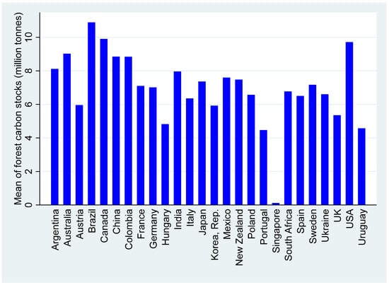
Figure 1.
Mean of forest carbon stocks (1996–2022).

Table 1.
Definitions and sources.
Table 2 reports the results of statistical tests for all selected variables, revealing that GDP has the highest mean value, with an average of 9.745, a minimum of 6.480, a maximum of 10.14, and a standard deviation of 1.047. The dependent variable, FCS, has a mean value 6.962, with a maximum of 10.95, a minimum of −0.034, and a standard deviation of 2.109. Among the independent variables, BE has the smallest mean value, with an average of 0.073, a minimum of 0.000, a maximum of 1.707, and a standard deviation of 0.231. The mean value for GAT is 3.708. The skewness test confirms that FCS, GDP, FD, and HC are negatively tailed variables, while both independent variables are positively tailed. According to the J–B test results, all variables in our model follow a non-normal distribution. The quantile–quantile (Q–Q) plots also show that our model’s variables are non-normal (see Figure 2).
Table 2.
Descriptive statistics.
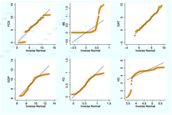
Figure 2.
Q–Q plots for normality.
Table 3 presents the estimates of the variance inflation factor (VIF) test for dependent, independent, and control variables, ensuring that there is no serious multicollinearity issue in the data. Table 3 displays the results of VIF test. According to this test, if the VIF score for any variable exceeds 5, it confirms the presence of a multicollinearity issue. As shown in Table 3, all the VIF values are less than 5, indicating that our dataset does not have a serious issue of multicollinearity. The mean VIF score is 1.78, which further confirms the absence of a multicollinearity issue in the data.
Table 3.
VIF results.
6. Empirical Analysis
6.1. Preliminary Results
Since panel data are used, preliminary tests are required prior to model estimation. These tests include a CSD test, a slope homogeneity test, a stationarity test, and a co-integration test. In the first step of the study, the Pesaran’s CSD test was performed, and the results are presented in Table 4. As shown in Table 4, all are variables are statistically significant. This confirms that the economies are cross-sectionally dependant on each other. Any shock that occurs in one economy will have an effect on other economies. The next step is to confirm the homogeneity of the slope of the variables. The study uses the Pesaran and Yamagata test to confirm the slope homogeneity of the variables. Table 5 summarizes the results of slope homogeneity test. Both delta and adjusted-delta parameters are significant, confirming that the slopes of the variables are heterogeneous. These findings confirm the presence of CSD and slope heterogeneity in the selected sample. The next step is to check the stationarity of the variables. To capture the CSD, second-generation unit root tests were employed in this study: the CADF and CIPS unit root tests. Table 6 shows the results of both unit root tests. According to the CIPS unit root test, BE, GAT, GDP, and FD are level stationary, while FCS and HC are stationary at the first difference. Meanwhile, in the CADF test, BE, GDP, and FD are level stationary, while the rest of the three variables (FCS, GAT, and HC) are first-difference stationary. In the final step, the study employs the Pedroni co-integration test to determine whether the variables are cointegrated in the long run. Table 7 displays the outcome of Pedroni co-integration test. These results indicate the presence of long-term co-integration among variables. It is confirmed that long-term co-integration relationship exists among FCS, BE, GAT, GDP, FD, and HC. After confirming the existence of long-term co-integration among the concerned variables, our study performs the MMQR test to examine the quantile association between FCS and the variables BE, GAT, GDP, FD, and HC. Table 8 shows the results obtained from the MMQR regression.
Table 4.
CSD results.
Table 5.
Slope heterogeneity results.
Table 6.
Unit root tests results.
Table 7.
Pedroni test for co-integration results.
Table 8.
MMQR results.
6.2. Empirical Results and Discussion
In Table 8, the MMQR results show that BE reveals a significantly positive influence on FCS across all quantiles, indicating the increasing effect of BE on forest carbon stocks. The magnitude of the effect is higher at the lowest quantile, which starts declining towards higher quantiles. The BE effect on FCS varies from 3.100 to 1.599 between the 0.10th quantile and the 0.90th quantile. This result is backed by Sedjo and Tian [55]. The connection between bioenergy and forest carbon stock is positive. Bioenergy is considered a low-carbon and reliable energy source that significantly reduces the amount of carbon concentration in the atmosphere. Bioenergy can enhance forest carbon stock if it is produced and managed through sustainable methods. For instance, producing bioenergy from forest remains, such as dead wood, is a more sustainable option than using and cutting down fresh, green forests. Moreover, bioenergy produced using special energy crops on previously unused land can significantly reduce the deforestation rate and help conserve forest resources, thereby increasing the availability of forests for carbon storage [56]. Furthermore, the sustainable production of bioenergy plays a crucial role in aligning existing forest management practices with sustainable ones, including thinning forests and removing unhealthy trees. Consequently, forest quality significantly improves, enhancing their capacity to store carbon. These empirical inferences are also supported by Favero et al. [57].
Conversely, MMQR reports a significant mitigating effect of GAT on FCS across almost all quantiles, from the 0.10th to the 0.80th quantiles. This confirms the positive role of GAT in reducing forest carbon stocks. However, the intensity of the effect is initially high at the lowest quantiles and declines at higher quantiles. At the 10th quantile, the magnitude of the effect is −2.398, declining to −0.619 at the 80th quantile. The nexus between GAT and FCS remains insignificant at the 0.90th quantile. Green agricultural technologies and forest carbon stocks are negatively linked, suggesting that the adoption of green agricultural technologies reduces forest carbon stocks. Although green agricultural technologies are intended to promote sustainable practices, inadequate management can undermine environmental quality and ultimately reduce forest carbon stocks. [58]. Despite the significance of green agricultural technologies in enhancing efficiency and mitigating environmental damage, their negative impact could be due to the following reasons: One of the key mechanisms behind the negative impact of green agricultural technologies on forest carbon stocks is the indirect effect resulting from land use change. This happens because green technologies play a vital role in enhancing total green productivity and boosting earnings from farming activities, resulting in a significant increase in the use of agricultural land by encroaching on forest areas. According to the Jeavons Paradox, increased technological development and efficiency may lead to a greater use of resources rather than their preservation [59]. Thus, green agricultural technologies significantly reduce the cost of production within the agricultural sector, enhancing total agricultural production and exerting more pressure on forest resources, thereby negatively impacting forest carbon stocks.
Green agricultural technologies are more likely to enhance per-acre yields, increasing farmers’ income and encouraging them to grow more crops on larger areas of land. As a result, the rate of deforestation significantly increases as farmers use more forest land to grow crops. In addition, the rising demand for organic agricultural products and foods encourages farmers to cultivate crops that take a long period to harvest and produce in low quantities, thus requiring more forest land to grow ample amounts of organic crops. Furthermore, in developing economies, the growth of green technologies primarily focuses on enhancing overall productivity in the agricultural sector without considering their ecological ramifications, leading to increased deforestation and reduced forest carbon stocks. These outcomes are also supported by Raihan et al. [60].
Among the control variables, the impact of GDP on FCS remains insignificant across all quantiles, indicating that GDP does not significantly influence the determination of forest carbon stocks. For FD, the MMQR reveals a significant positive effect of FD on FCS across all quantiles. This positive nexus between FD and FCS indicates an increasing effect of financial development on forest carbon stocks. Financial development enhances access to finance for sustainable landscape projects, which aim to achieve deforestation-free and community-based forestry development. A similar result is also reported by Dong et al. [61], who found that green financial development is essential for the growth of the forestry sector in China. Lastly, the MMQR results show a significant negative relationship between HC and FCS across all quantiles, indicating that human capital tends to reduce forest capital stock. The possible reason is that increased human capital indicates the economy is in a transition phase from an agricultural to an industrial sector, enhancing economic activity, infrastructure development, and land use changes, as well as urbanization. These activities can significantly reduce forest areas in the initial phases, particularly in regions where ecological regulations are weak [62]. However, the magnitude of the effect declines from the lowest to the highest quantiles. The coefficient of HC is −0.999 at the 10th quantile, which reduces to −0.616 at the 10th quantile. The graphical MMQR results are presented in Figure 3.
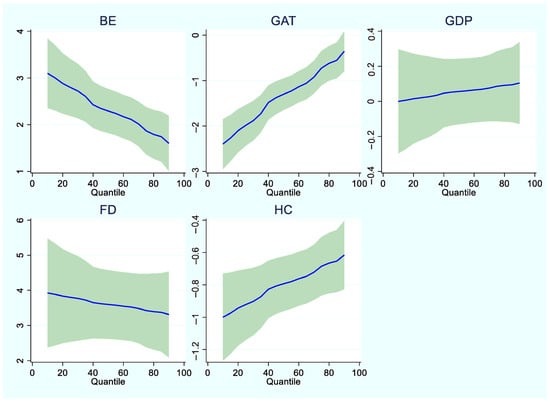
Figure 3.
MMQR results.
6.3. Robustness Results
To confirm the robustness of the MMQR results, our study employed the FMOLS and DCCE methods. Table 9 reports the estimates of FMOLS and DCCE regressions. The results from FMOLS and DCCE indicate a significant positive effect of BE on FCS, indicating a detrimental effect of bioenergy on forest carbon stocks. It is noted that a 1% upsurge in BE is attached with a 2.960% increment in FCS under FMOLS and 1.095% upsurge in FCS under DCCE. GAT, on the other hand, reports a significantly negative connection with FCS in FMOLS only, showing that green agricultural technologies tend to reduce forest carbon stock. The GAT coefficient estimate is −0.101, indicating that a 1% rise in GAT reduces FCS by 0.101% under FMOLS. Conversely, the nexus between GAT and FCS is statistically insignificant under DCCE. The results from FMOLS indicate that GDP has a significant and positive effect on FCS. This suggests that higher GDP leads to higher forest carbon stocks. A 1% rise in GDP tends to escalate FCS by 0.171% under FMOLS. However, the linkage between GDP and FCS is reported as positive, but the nature of the effect is insignificant under DCCE. Similarly, the results from FMOLS and DCCE show that FD has a significant and positive effect on FCS, indicating that higher financial development exacerbates forest carbon stocks. A 1% improvement in FD enhances FCS by 1.554% under FMOLS and 1.025% under DCCE. Lastly, HC shows a significantly negative linkage with FCS under FMOLS, confirming the positive role of human capital in reducing forest carbon stocks. A 1% upsurge in HC reports 0.215% reduction in FCS under FMOLS. The association between HC and FCS is reported to be insignificant under DCCE.
Table 9.
FMOLS and DCCE estimates.
6.4. Long- and Short-Term Results
In Table 10, our study employed the CS-ARDL and PM-ARDL approaches to investigate the long-term and short-term results. According to the long-term estimated results, it is evident that a 1% rise in BE produces a 1.322% increase in FCS under CS-ARDL and a 2.167% upsurge in FCE under PM-ARDL over the long term. This indicates that bioenergy has a positive impact on forest carbon stocks in our analysis. On the other hand, a negative and significant relationship between GAT and FCS is confirmed in both models in the long run. Our findings reveal that a 1% increase in GAT has resulted in a 0.005% reduction in FCS under CS-ARDL and a 0.010% reduction in FCS under PARDL. This shows a positive contribution of green agricultural technologies in reducing forest carbon stocks. The nexus between GDP and FCS is significantly positive in the CS-ARDL only in the long run. Empirical research shows that a 1% enhancement in GDP enhances FCS by 0.330% in the long term. FD has a significantly positive correlation with FCS in the PM-ARDL regression. In the long run, a 1% increase in financial development leads to a 0.089% increase in forest carbon stocks. Finally, HC estimates are insignificant in both models, indicating that human capital does not play a role in determining forest carbon stocks.
Table 10.
Long- and short-term estimates.
In the short term, D(BE) exhibits a significantly positive impact on FCS in the PM-ARDL. Whereas the D(GAT) association with FCS is found to be statistically insignificant in both models. Among the control variables, D(GDP) shows a significantly positive correlation with FCS in both models in the short term. The impact of D(FD) and D(HC) is found to be insignificant in both models in the short term. Lastly, the ECM(−1) estimates are significantly negative in both models, confirming the tendency for both models to converge towards equilibrium. According to the estimates, 77% convergence is expected to occur within one year under the CS-ARDL model, and 50% convergence is anticipated in one year under the PM-ARDL model.
6.5. Developed and Developing Economies Results
The study also conducted disaggregated analysis for developed and developing economies. Table 11 displays the MMQR estimates for developed economies. The MMQR results reveal that BE exerts a significantly positive impact on FCS at medium and higher quantiles, from the 0.50th quantile to the 0.80th quantile. It demonstrates that increased bioenergy exaggerates forest carbon stock in developed economies. The intensity of this effect is strongest at the medium quantiles and gradually declines toward the higher quantiles. However, the linkage between BE and FCS remains insignificant at lower and highest quantiles, ranging from the 0.10th to the 0.40th quantiles and the 0.90th quantile. Conversely, GAT exhibits a significantly negative linkage with FCS from medium to higher quantiles, specifically from the 0.50th to 0.80th quantiles. The relationship between GAT and FCS becomes statistically insignificant at the lower and highest quantiles, ranging from the 0.10th to the 0.40th quantile and the 0.90th quantile. In the case of control variables, GDP exerts a significantly positive impact on FCS at highest quantiles only, from the 0.70th quantile to the 0.90th quantile. It shows that increased GDP can exaggerate forest carbon stocks in developed economies. However, the linkage between GDP and FCS remains insignificant at lower and medium quantiles, ranging from the 0.10th to the 0.60th quantiles. On the other hand, FD does not report any statistically significant impact on forest carbon stocks across all quantiles. Lastly, HC reveals a significant negative effect on FCS from the 0.10th quantile to the 0.40th quantile, implying that improvements in human capital are associated with reduced forest carbon stocks in developed economies. However, HC exhibits no impact on FCS from 0.50th to 0.90th quantiles.
Table 11.
MMQR results (developed countries).
Table 12 presents the MMQR estimates for developing economies. The results indicate that BE has a significantly positive impact on FCS across all quantiles from the 0.10th to the 0.90th quantile. The highly significant positive influence of bioenergy on forest carbon stocks in developing countries suggests that bioenergy in these economies primarily relies on agricultural waste, crop residues, and other sustainable methods of generation, thereby significantly reducing the reliance on fresh forest resources for bioenergy production. Further, the positive influence also shows the increased reliance of these economies on bioenergy sources, while the insignificant influence of bioenergy on forest carbon stocks in the developed economies is an indication of the less reliance on bioenergy sources and the reliance on other renewable and low-carbon energy sources, including solar, wind, hydel, and nuclear energy. Conversely, GAT exhibits a significantly negative connection with FCS from the 0.10th to the 0.50th quantile. From the 0.60th to 0.90th quantiles, this relationship becomes insignificant, indicating no effect of green agricultural technologies on forest carbon stocks. GDP also shows a significant negative impact on FCS from the 0.10th to the 0.50th quantiles, indicating that GDP substantially reduces forest carbon stocks in developing countries. Although the effect is higher at lower quantiles and declines gradually from medium to higher quantiles, the nexus between GDP and FCS is reported to be statistically insignificant at the highest quantiles (the 0.60th and 0.90th quantiles). On the other hand, FD demonstrates no significant effect across all quantiles. HC reveals a significant negative impact on FCS across all quantiles. These findings suggest that improvements in human capital are significantly linked to reductions in forest carbon stocks in developing economies.
Table 12.
MMQR results (developing countries).
7. Conclusions, Policy Recommendations, and Future Directions
Forests play a pivotal role in maintaining balance within the ecosystem. One of the most significant ecosystem services provided by forests is their ability to sequester carbon. However, rapid deforestation can significantly reduce the forest carbon stocks or their ability to sequester carbon. The protection of existing forests and the growth of new forests are crucial for enhancing forest carbon stocks. Enhancing the forest carbon stocks is crucial for mitigating climate change and global warming. Given the significance of carbon stocks for improving environmental quality, academics and empirical studies have shown a growing interest in identifying the factors that can enhance forests’ ability to store more carbon. In recent times, bioenergy has regained popularity as a low-carbon and sustainable energy source. Particularly, the bioenergy produced from using plant residues and dead wood can reduce the strain on forest resources and positively influence the carbon stock in forests. However, if bioenergy is produced by cutting down green forests, it can harm the forest’s carbon stocks. Similarly, agricultural technologies and practices, when effectively implemented, can substantially enhance forest carbon stocks; however, unsustainable management may result in their depletion. Due to the complex nature of the relationship between bioenergy, agriculture technologies, and forest carbon, it is crucial to understand the influence of bioenergy and agriculture technologies on forest carbon stocks. Thus, the primary objective of this analysis is to investigate the impact of bioenergy and agricultural technologies on forest carbon stocks. Additionally, the study conducted a comparative analysis between developed and developing economies.
To that end, the novel MMQR technique is employed. Findings from the MMQR technique indicate a positive correlation between bioenergy and forest carbon stocks across the 10th to 90th quantiles, confirming that bioenergy has been beneficial in enhancing forest carbon stocks at all levels. In the case of developing economies, similar results are identified; however, for developed economies, a positive association between bioenergy and forest carbon stocks is observed at the lower and medium quantiles (i.e., from the 10th to the 50th percentile). On the other hand, a negative linkage is observed between agricultural technologies and forest carbon stocks at all quantiles, i.e., from the 10th to the 90th quantiles, implying that green agricultural technologies are detrimental to forest carbon stocks. In both developed and developing economies, a negative linkage is also observed between agricultural technologies and forest carbon stocks at most quantiles, except for the higher quantiles in developed economies. In addition, the GDP has a negative influence on forest carbon stocks only in developing economies, whereas human capital has a negative influence on forest carbon stocks in both developed and developing economies.
In light of these findings, several policy recommendations are presented. First and foremost, the varying influence of bioenergy and green agricultural technologies on forest carbon stocks confirms the asymmetric connection between them. Thus, policymakers should consider these asymmetric impacts while devising policies for the protection of the ecosystem and enhancing the ability of the forests to store carbon. Bioenergy is a crucial factor in enchanting forest carbon stocks. Policymakers should focus on enhancing the production of bioenergy in the overall energy mix, which will not only improve forest carbon stocks but also address issues related to energy security and helping economies grow sustainably. Moreover, it is also suggested that policymakers encourage the production of bioenergy by utilising forest residues, dead wood, and non-food crops, which would help conserve forest resources and enhance forest carbon stocks. Furthermore, the results indicate that the government should increase R&D spending for the production of bioenergy from alternative resources (e.g., crop residues, industrial residues, solid waste, and cow dung) rather than directly burning forest resources. The results suggested that policymakers should focus on using leftover crop materials, such as “straw, husks, or sugarcane residues and animal waste” for bioenergy. Particularly, policymakers should avoid the large-scale cultivation of energy-specific crops, such as palm oil and maize, for the production of biofuels, which can lead to the replacement of more forest land, thereby enhancing deforestation and reducing carbon stocks in forests. In this way, forests can be protected from the negative impacts of bioenergy generation, thereby increasing total forest cover and enhancing the ability of forests to absorb more carbon.
Green agricultural technologies are detrimental to forest carbon stocks. Thus, policymakers should devise stringent environmental policies that discourage the cutting of forests and trees, while promoting the use of green agricultural technologies. Moreover, the government should support and encourage the growth of agriculture and farming activities on previously unused or barren land, rather than on forest land. To ensure food security and forest protection, the government should encourage the cultivation of multiple crops instead of single crops that require large areas of land and which threaten food security. The government should also encourage the use of digital technologies to integrate activities within the agriculture and forestry sectors, which are crucial for tracking forest and agricultural activities in real-time and helping to preserve forests without compromising food security objectives. Furthermore, the results suggest that the government exercise caution when increasing the share of bioenergy and investing in green agricultural technologies, as there may be a potential trade-off associated with enhanced bioenergy production. For instance, enhancing bioenergy and employing green agricultural technologies can increase agriculture-related activities, potentially leading to increased land use. On one hand, due to increased land usage for agricultural activities, the overall food supply and bioenergy production are significantly improved; on the other hand, excessive land use can prove detrimental to the ecosystem. Thus, the policymakers should integrate the objectives of bioenergy production, food security, and environmental protection into economic and environmental policies. Lastly, developed and developing economies should coordinate and benefit from each other’s experiences. For instance, bioenergy is proving more efficient in developing economies instead in developed ones in enhancing forest carbon stocks. In this regard, developed economies should learn from the experiences of developing economies and focus on increasing the share of bioenergy in their total energy mix. On the other hand, developed and developing economies should coordinate and support each other in ensuring that green technologies more aligned with ecological objectives.
Indeed, the studies have contributed to the available literature in several ways; however, some limitations are worth mentioning. Primarily, the studies have omitted some important variables, such as environmental policy stringency, energy consumption, urbanization, and industrialization that are important drivers of environmental quality and may influence forest carbon stocks. Due to methodological limitations, some econometric models used in this study do not allow the inclusion of more than six variables in single model. Therefore, a separate study should be conducted focusing on these variables. Due to the unavailability of environmental education data for the sample economies, this study used human capital as a control variable in the analysis. Moreover, it is acknowledged that the human capital proxy may not fully capture qualitative aspects, such as environmental awareness. Future research is encouraged to explore alternative measures, including environmental education. Lastly, the future analysis should also focus on the causal relationship between bioenergy, green agricultural technologies, and forest carbon stocks to inform more effective policy suggestions. Additionally, if data become available, future studies can expand the sample or conduct subregional analyses (e.g., by continent or forest type) that could reveal additional heterogeneity and increase generalizability.
Author Contributions
N.H.D.L.: conceptualization, methodology, writing—original draft, formal analysis. L.L.: data curation, software, writing—original draft, editing, and proofreading. All authors have read and agreed to the published version of the manuscript.
Funding
This research received no external funding.
Data Availability Statement
Data are available on reasonable request to the corresponding author.
Conflicts of Interest
The authors declare no conflicts of interest.
Appendix A
Table A1.
Sample countries.
Table A1.
Sample countries.
| Developed Countries | Developing Countries |
|---|---|
| Singapore | Brazil |
| France | Mexico |
| Germany | Argentina |
| Sweden | Colombia |
| Austria | Ukraine |
| Spain | Uruguay |
| New Zealand | India |
| Portugal | China |
| UK | South Africa |
| Australia | |
| Korea, Rep. | |
| USA | |
| Japan | |
| Canada | |
| Italy | |
| Hungary | |
| Poland |
References
- Nunes, L.J.; Meireles, C.I.; Gomes, C.J.P.; Ribeiro, N.M.A. Forest contribution to climate change mitigation: Management oriented to carbon capture and storage. Climate 2020, 8, 21. [Google Scholar] [CrossRef]
- USGS. What Is Carbon Sequestration? 2025. Available online: https://www.usgs.gov/faqs/what-carbon-sequestration (accessed on 27 July 2025).
- IPCC. Special Report on Climate Change and Land 2019. Available online: https://www.ipcc.ch/site/assets/uploads/2019/11/SRCCL-Full-Report-Compiled-191128.pdf (accessed on 27 July 2025).
- Zeng, N.; King, A.W.; Zaitchik, B.; Wullschleger, S.D.; Gregg, J.; Wang, S.; Kirk-Davidoff, D. Carbon sequestration via wood harvest and storage: An assessment of its harvest potential. Clim. Chang. 2013, 118, 245–257. [Google Scholar] [CrossRef]
- Pingoud, K.; Ekholm, T.; Sievänen, R.; Huuskonen, S.; Hynynen, J. Trade-offs between forest carbon stocks and harvests in a steady state—A multi-criteria analysis. J. Environ. Manag. 2018, 210, 96–103. [Google Scholar] [CrossRef] [PubMed]
- Berndes, G.; Abt, B.; Asikainen, A.; Cowie, A.; Dale, V.; Egnell, G.; Lindner, M.; Marelli, L.; Paré, D.; Pingoud, K.; et al. Forest biomass, carbon neutrality and climate change mitigation. Sci. Policy 2016, 3, 1–27. [Google Scholar]
- Adhikari, D.; Singh, P.P.; Tiwary, R.; Barik, S.K. Forest carbon stock-based bioeconomy: Mixed models improve accuracy of tree biomass estimates. Biomass Bioenergy 2024, 183, 107142. [Google Scholar] [CrossRef]
- PIB. The Rise of India’s Bioeconomy from $10bn to $165.75bn in a Decade. 2025. Available online: https://www.pib.gov.in/PressReleasePage.aspx?PRID=2115882 (accessed on 27 July 2025).
- Tavoni, M.; Sohngen, B.; Bosetti, V. Forestry and the carbon market response to stabilize climate. Energy Policy 2007, 35, 5346–5353. [Google Scholar] [CrossRef]
- Cambero, C.; Sowlati, T. Assessment and optimization of forest biomass supply chains from economic, social and environmental perspectives—A review of literature. Renew. Sustain. Energy Rev. 2014, 36, 62–73. [Google Scholar] [CrossRef]
- EPA. Global Greenhouse Gas Overview. Available online: https://www.epa.gov/ghgemissions/global-greenhouse-gas-overview (accessed on 27 July 2025).
- Shaheen, F.; Lodhi, M.S.; Rosak-Szyrocka, J.; Zaman, K.; Awan, U.; Asif, M.; Ahmed, W.; Siddique, M. Cleaner technology and natural resource management: An environmental sustainability perspective from China. Clean Technol. 2022, 4, 584–606. [Google Scholar] [CrossRef]
- Zhang, C.; Liu, C. The impact of ICT industry on CO2 emissions: A regional analysis in China. Renew. Sustain. Energy Rev. 2015, 44, 12–19. [Google Scholar] [CrossRef]
- Farooq, S.; Ozturk, I.; Majeed, M.T.; Akram, R. Globalization and CO2 emissions in the presence of EKC: A global panel data analysis. Gondwana Res. 2022, 106, 367–378. [Google Scholar] [CrossRef]
- Bilgili, F.; Koçak, E.; Bulut, U. The dynamic impact of renewable energy consumption on CO2 emissions: A revisited Environmental Kuznets Curve approach. Renew. Sustain. Energy Rev. 2016, 54, 838–845. [Google Scholar] [CrossRef]
- Martínez-Zarzoso, I.; Maruotti, A. The impact of urbanization on CO2 emissions: Evidence from developing countries. Ecol. Econ. 2011, 70, 1344–1353. [Google Scholar] [CrossRef]
- Apeaning, R.W.; Labaran, M. Does financial development moderate the impact of climate mitigation innovation on CO2 emissions? Evidence from emerging economics. Innov. Green Dev. 2025, 4, 100211. [Google Scholar] [CrossRef]
- He, P.; Zhang, J.; Li, W. The role of agricultural green production technologies in improving low-carbon efficiency in China: Necessary but not effective. J. Environ. Manag. 2021, 293, 112837. [Google Scholar] [CrossRef]
- Villoria, N.B.; Byerlee, D.; Stevenson, J. The effects of agricultural technological progress on deforestation: What do we really know? Appl. Econ. Perspect. Policy 2014, 36, 211–237. [Google Scholar] [CrossRef]
- D’Amato, A.; Mazzanti, M.; Nicolli, F. Green technologies and environmental policies for sustainable development: Testing direct and indirect impacts. J. Clean. Prod. 2021, 309, 127060. [Google Scholar] [CrossRef]
- Khan, A.N.; En, X.; Raza, M.Y.; Khan, N.A.; Ali, A. Sectorial study of technological progress and CO2 emission: Insights from a developing economy. Technol. Forecast. Soc. Chang. 2020, 151, 119862. [Google Scholar] [CrossRef]
- Hrubovcak, J. Green Technologies for a More Sustainable Agriculture; Economic Research Service, US Department of Agriculture: Washington, DC, USA, 1999. [Google Scholar]
- Guo, Z.; Zhang, X. Carbon reduction effect of agricultural green production technology: A new evidence from China. Sci. Total. Environ. 2023, 874, 162483. [Google Scholar] [CrossRef]
- Destek, M.A.; Sarkodie, S.A.; Asamoah, E.F. Does biomass energy drive environmental sustainability? An SDG perspective for top five biomass consuming countries. Biomass Bioenergy 2021, 149, 106076. [Google Scholar] [CrossRef]
- FAO. Wood Energy and Non-Wood Forest Products Play Major Roles in the Majority of Rural Households. 2022. Available online: https://openknowledge.fao.org/server/api/core/bitstreams/8f599970-661d-45f5-a598-2ea46ca1605f/content/src/html/wood-products-energy-households.html#note-75 (accessed on 27 July 2025).
- Letti, L.A.J.; Sydney, E.B.; de Carvalho, J.C.; de Souza Vandenberghe, L.P.; Karp, S.G.; Woiciechowski, A.L.; Soccol, V.T.; Novak, A.C.; Junior, A.I.M.; Burgos, W.J.M. Roles and impacts of bioethanol and biodiesel on climate change mitigation. In Biomass, Biofuels, Biochemicals; Elsevier: Amsterdam, The Netherlands, 2022; pp. 373–400. [Google Scholar]
- Kanianska, R. Agriculture and its impact on land-use, environment, and ecosystem services. In Landscape Ecology-The Influences of Land Use and Anthropogenic Impacts of Landscape Creation; IntechOpen: London, UK, 2016; pp. 1–26. [Google Scholar]
- Marshall, E.; Caswll, M.; Malcolm, S.; Motamed, M.; Hrubovcak, J.; Jones, C.; Nickerson, C. Measuring the Indirect Land-Use Change Associated with Increased Biofuel Feedstock Production: A Review of Modeling Efforts: Report to Congress; United States Department of Agriculture (USDA): Washington, DC, USA, 2011. [Google Scholar]
- Soto, J.R.; Escobedo, F.J.; Adams, D.C.; Blanco, G. A distributional analysis of the socio-ecological and economic determinants of forest carbon stocks. Environ. Sci. Policy 2016, 60, 28–37. [Google Scholar] [CrossRef]
- Meeussen, C.; Govaert, S.; Vanneste, T.; Haesen, S.; Van Meerbeek, K.; Bollmann, K.; Brunet, J.; Calders, K.; Cousins, S.A.; Diekmann, M.; et al. Drivers of carbon stocks in forest edges across Europe. Sci. Total Environ. 2021, 759, 143497. [Google Scholar] [CrossRef]
- De Hoyos, R.E.; Sarafidis, V. Testing for cross-sectional dependence in panel-data models. Stata J. 2006, 6, 482–496. [Google Scholar] [CrossRef]
- Usman, M.; Anwar, S.; Yaseen, M.R.; Makhdum, M.S.A.; Kousar, R.; Jahanger, A. Unveiling the dynamic relationship between agriculture value addition, energy utilization, tourism and environmental degradation in South Asia. J. Public Aff. 2022, 22, e2712. [Google Scholar] [CrossRef]
- Amin, N.; Song, H. The role of renewable, non-renewable energy consumption, trade, economic growth, and urbanization in achieving carbon neutrality: A comparative study for South and East Asian countries. Environ. Sci. Pollut. Res. 2023, 30, 12798–12812. [Google Scholar] [CrossRef] [PubMed]
- Pesaran, M. General Diagnostic Tests for Cross Section Dependence in Panels (No. 1240); Institute of Labor Economics (IZA): Bonn, Germany, 2004. [Google Scholar]
- Pesaran, M.H.; Yamagata, T. Testing slope homogeneity in large panels. J. Econ. 2008, 142, 50–93. [Google Scholar] [CrossRef]
- Maddala, G.S.; Wu, S. A comparative study of unit root tests with panel data and a new simple test. Oxf. Bull. Econ. Stat. 1999, 61, 631–652. [Google Scholar] [CrossRef]
- Choi, I. Unit root tests for panel data. J. Int. Money Financ. 2001, 20, 249–272. [Google Scholar] [CrossRef]
- Bai, J.; Ng, S. A PANIC Attack on unit roots and cointegration. Econometrica 2004, 72, 1127–1177. [Google Scholar] [CrossRef]
- Pesaran, M.H. A simple panel unit root test in the presence of cross-section dependence. J. Appl. Econ. 2007, 22, 265–312. [Google Scholar] [CrossRef]
- Pedroni, P. Panel cointegration: Asymptotic and finite sample properties of pooled time series tests with an application to the PPP hypothesis. Econom. Theory 2004, 20, 597–625. [Google Scholar] [CrossRef]
- Koenker, R.; Bassett, G., Jr. Regression quantiles. Econom. J. Econom. Soc. 1978, 46, 33–50. [Google Scholar] [CrossRef]
- Mohammed, K.S.; Mellit, A. The relationship between oil prices and the indices of renewable energy and technology companies based on QQR and GCQ techniques. Renew. Energy 2023, 209, 97–105. [Google Scholar] [CrossRef]
- Chang, L.; Lu, Q.; Ali, S.; Mohsin, M. How does hydropower energy asymmetrically affect environmental quality? Evidence from quantile-based econometric estimation. Sustain. Energy Technol. Assess. 2022, 53, 102564. [Google Scholar] [CrossRef]
- Machado, J.A.; Silva, J.S. Quantiles via moments. J. Econom. 2019, 213, 145–173. [Google Scholar] [CrossRef]
- Basheer, M.F.; Anwar, A.; Hassan, S.G.; Alsedrah, I.T.; Cong, P.T. Does financial sector is helpful for curbing carbon emissions through the investment in green energy projects: Evidence from MMQR approach. Clean Technol. Environ. Policy 2023, 26, 901–921. [Google Scholar] [CrossRef]
- Phillips, P.C.B.; Hansen, B.E. Statistical inference in instrumental variables regression with I(1) processes. Rev. Econ. Stud. 1990, 57, 99–125. [Google Scholar] [CrossRef]
- Chudik, A.; Pesaran, M.H. Common correlated effects estimation of heterogeneous dynamic panel data models with weakly exogenous regressors. J. Econ. 2015, 188, 393–420. [Google Scholar] [CrossRef]
- Arain, H.; Han, L.; Meo, M.S. Nexus of FDI, population, energy production, and water resources in South Asia: A fresh insight from dynamic common correlated effects (DCCE). Environ. Sci. Pollut. Res. 2019, 26, 27128–27137. [Google Scholar] [CrossRef] [PubMed]
- Sohail, M.T.; Ullah, S.; Sohail, S. Environmental sustainability: The role of mineral resources trade and private investment. Miner. Econ. 2025. online first. [Google Scholar] [CrossRef]
- Wang, L.; Wei, Y.; Li, B.; Zheng, S.; Ullah, S.; Sohail, S. Renewable energy consumption and its impacts on agriculturalization under climate neutrality targets. Energy Environ. 2024. online first. [Google Scholar] [CrossRef]
- Sohail, M.T.; Li, W.; Sohail, S. Greening the Economy: How Forest-Product Trade and Bioenergy Shape the Framework for Green Growth. Forests 2024, 15, 1960. [Google Scholar] [CrossRef]
- Hötte, K.; Jee, S.J. Knowledge for a warmer world: A patent analysis of climate change adaptation technologies. Technol. Forecast. Soc. Chang. 2022, 183, 121879. [Google Scholar] [CrossRef]
- Ewers, R.M. Interaction effects between economic development and forest cover determine deforestation rates. Glob. Environ. Chang. 2006, 16, 161–169. [Google Scholar] [CrossRef]
- Thathong, K.; Leopenwong, S. The development of environmental education activities for forest resources conservation for the youth. Procedia Soc. Behav. Sci. 2014, 116, 2266–2269. [Google Scholar] [CrossRef][Green Version]
- Sedjo, R.; Tian, X. Does wood bioenergy increase carbon stocks in forests? J. For. 2012, 110, 304–311. [Google Scholar] [CrossRef]
- Calvin, K.; Cowie, A.; Berndes, G.; Arneth, A.; Cherubini, F.; Portugal-Pereira, J.; Grassi, G.; House, J.; Johnson, F.X.; Popp, A. Bioenergy for climate change mitigation: Scale and sustainability. GCB Bioenergy 2021, 13, 1346–1371. [Google Scholar] [CrossRef]
- Favero, A.; Daigneault, A.; Sohngen, B. Forests: Carbon sequestration, biomass energy, or both? Sci. Adv. 2020, 6, eaay6792. [Google Scholar] [CrossRef]
- De Corato, U.; Viola, E.; Keswani, C.; Minkina, T. Impact of the sustainable agricultural practices for governing soil health from the perspective of a rising agri-based circular bioeconomy. Appl. Soil Ecol. 2024, 194, 105199. [Google Scholar] [CrossRef]
- Sears, L.; Caparelli, J.; Lee, C.; Pan, D.; Strandberg, G.; Vuu, L.; Lin Lawell, C.-Y. Jevons’ paradox and efficient irrigation technology. Sustainability 2018, 10, 1590. [Google Scholar] [CrossRef]
- Raihan, A.; Pavel, M.I.; Muhtasim, D.A.; Farhana, S.; Faruk, O.; Paul, A. The role of renewable energy use, technological innovation, and forest cover toward green development: Evidence from Indonesia. Innov. Green Dev. 2023, 2, 100035. [Google Scholar] [CrossRef]
- Dong, B.; Chen, L.; Zhang, Y.; Xie, B. How does green credit supply enhance the efficiency of forestry ecological development? Taking the perspective of ecological total factor productivity. J. Clean. Prod. 2025, 488, 144643. [Google Scholar] [CrossRef]
- Jiang, Y.; Wang, Y.; Wang, R. Coupling and Coordination Relationship between Economic and Ecologic-Environmental Developments in China’s Key State-Owned Forest Areas. Sustainability 2022, 14, 15899. [Google Scholar] [CrossRef]
Disclaimer/Publisher’s Note: The statements, opinions and data contained in all publications are solely those of the individual author(s) and contributor(s) and not of MDPI and/or the editor(s). MDPI and/or the editor(s) disclaim responsibility for any injury to people or property resulting from any ideas, methods, instructions or products referred to in the content. |
© 2025 by the authors. Licensee MDPI, Basel, Switzerland. This article is an open access article distributed under the terms and conditions of the Creative Commons Attribution (CC BY) license (https://creativecommons.org/licenses/by/4.0/).