Article

Kennaugh Elements Allow Early Detection of Bark Beetle Infestation in Temperate Forests Using Sentinel-1 Data

1
Geoinformatics Department, Munich University of Applied Sciences (HM), Karlstraße 6, 80333 Munich, Germany
2
Institute for Applications of Machine Learning and Intelligent Systems (IAMLIS), Munich University of Applied Sciences (HM), Lothstraße 34, 80335 Munich, Germany
3
Department of National Park Monitoring and Animal Management, Bavarian Forest National Park, Freyunger Straße 2, D-94481 Grafenau, Germany
4
Wildlife Ecology and Management, University of Freiburg, Tennenbacher Straße 4, 79106 Freiburg, Germany
5
Institute for Forest and Wildlife Management, Campus Evenstad, University of Inland Norway, 2480 Koppang, Norway
6
Earth Observation Center (EOC), German Aerospace Center (DLR), Oberpfaffenhofen, 82234 Weßling, Germany
*
Author to whom correspondence should be addressed.
Forests 2025, 16(8), 1272; https://doi.org/10.3390/f16081272 (registering DOI)
Submission received: 3 July 2025 / Revised: 25 July 2025 / Accepted: 30 July 2025 / Published: 3 August 2025
(This article belongs to the Section Forest Health)

Abstract

Climate change is generally having a negative impact on forest health by inducing drought stress and favouring the spread of pest species, such as bark beetles. The terrestrial monitoring of bark beetle infestation is very time-consuming, especially in the early stages, and therefore not feasible for extensive areas, emphasising the need for a comprehensive approach based on remote sensing. Although numerous studies have researched the use of optical data for this task, radar data remains comparatively underexplored. Therefore, this study uses the weekly and cloud-free acquisitions of Sentinel-1 in the Bavarian Forest National Park. Time series analysis within a Multi-SAR framework using Random Forest enables the monitoring of moisture content loss and, consequently, the assessment of tree vitality, which is crucial for the detection of stress conditions conducive to bark beetle outbreaks. High accuracies are achieved in predicting future bark beetle infestation (R2 of 0.83–0.89). These results demonstrate that forest vitality trends ranging from healthy to bark beetle-affected states can be mapped, supporting early intervention strategies. The standard deviation of 0.44 to 0.76 years indicates that the model deviates on average by half a year, mainly due to the uncertainty in the reference data. This temporal uncertainty is acceptable, as half a year provides a sufficient window to identify stressed forest areas and implement targeted management actions before bark beetle damage occurs. The successful application of this technique to extensive test sites in the state of North Rhine-Westphalia proves its transferability. For the first time, the results clearly demonstrate the expected relationship between radar backscatter expressed in the Kennaugh elements K0 and K1 and bark beetle infestation, thereby providing an opportunity for the continuous and cost-effective monitoring of forest health from space.

1. Introduction

The Sentinel missions in the Copernicus programme of the European Space Agency (ESA) enable large-scale forest monitoring with high spatial, temporal and spectral resolution, supporting sustainable forest management and the preservation of biodiversity and ecosystem services [1,2]. In the era of climate change, applying these spaceborne sensors is essential to inform forest management, as terrestrial data collection with high spatial and temporal resolutions is no longer applicable [3,4]. Extreme events caused by global warming, such as windthrow, prolonged droughts, and increasing biotic disturbances, are threatening forests and altering their ecological dynamics. These changing environmental conditions favour the spread of insects such as the Norway spruce bark beetle (Ips typographus (L.)), currently recognised as the most significant pest species in European forests [5,6]. Norway spruce trees (Picea abies (L.) Karst.), weakened by higher temperatures and drought, can no longer defend themselves sufficiently against the insects and will die when infested [7]. The recent surge in forest disturbances poses a major challenge for forest managers, particularly in preventing insect outbreaks such as those caused by bark beetles [8,9,10]. Reliable information on forest conditions and changes forms the basis for timely countermeasures and is therefore crucial [11]. To address these issues, field surveys can detect early signs of bark beetle infestation, such as boring dust, and bark beetles themselves can be captured using pheromone traps [12,13]. While these methods provide valuable insights at a local scale, they are limited in their spatial coverage and scalability. Due to the large spatial extent of the disturbances and the need for a quick response, terrestrial data collection is no longer feasible. Species distribution models, such as Maximum Entropy modelling, incorporate environmental and topographical variables to predict the potential spread [13,14]. However, they require careful calibration, as initial parameter settings and spatial biases in occurrence data can significantly influence model performance. Consequently, a high level of expertise is essential to ensure the robustness and reliability of the modelling results [14]. Moreover, MaxEnt models are inherently limited by their reliance on presence-only data and, in most cases, on long-term environmental averages. This means they often fail to reflect current conditions or short-term ecological dynamics. These limitations underscore the growing importance of remote sensing approaches. Unlike terrestrial methods that require the installation and maintenance of traps or ground surveys remote sensing allows for comprehensive, landscape-wide assessments without the need for physical sampling, making it invaluable for detecting and managing insect driven disturbances over vast and often inaccessible areas.
Given these challenges, effective remote sensing applications must account for the swarming behaviour of bark beetles and their interactions with trees. Ips typographus typically begin swarming after approximately 47 warm days, usually around mid-April when temperatures rise above 16.5 °C [15]. Subsequently, they bore into spruce trees to lay eggs. [5,15,16]. After 6 to 10 weeks [12], a new generation matures and initiates another infestation cycle. Warm and dry years allow a bark beetle season from April to around mid-September during which up to three generations can develop in addition to the sibling broods. In cooler regions, such as Scandinavia typically only one generation develops, with a second generation occurring occasionally [17,18]. Bark beetle-infested trees exhibit a range of symptoms [12,19]. Freshly infested trees exhibit subtle symptoms such as boring dust, resin flow, and minor bark loss, known as the “green attack stage”, during which foliage remains green. Early detection and removal at this stage are critical to preventing the next generation of bark beetles. As the infestation progresses, significant bark loss occurs, accompanied by the shedding of green and yellowish needles and the reddish discolouration of the crown, known as a “red attack stage” [12]. This indicates that the tree is dying or has already died. The final state the “grey attack stage”, in which the tree is already dead, has lost its needles and only the bare branches and a lifeless crown remain. While the advanced stages of infestation, red attack and grey attack, can be reliably detected by optical sensor systems due to their clearly visible symptoms, the detection of the green attack stage poses still a challenge [12]. Since the forest is a complex ecosystem, many other factors, such as available breeding material or water availability, play a crucial role in the bark beetle infestation process. During infestation, stomatal conductivity decreases as trees close their stomata to reduce water loss, leading to reduced photosynthesis and transpiration. This also results in increased needle surface temperatures [19]. These different characteristics between infested and healthy spruce trees are utilised in remote sensing to detect bark beetle attacks [20,21]. A field study demonstrated that the change of leaf characteristics in the early stages of infestation, which is not visible to the human eye, can be measured using a chlorophyll content meter and a field spectrometer. In infested spruce trees, both the chlorophyll and water content of the needles decrease, while the dry matter content increases [22]. Based on these findings our study hypothesises that the decrease in water content is visible in temporal combinations of radar images from space, because Synthetic Aperture Radar (SAR) technology is sensitive to the dielectric properties of the imaged targets: the higher the water content, the higher the scattering [23,24,25]. Infected trees are thus expected to show a slightly lower backscatter than healthy trees, and the green attack stage should, therefore, be identifiable at an early stage.

1.1. Remote Detection of Bark Beetle Infestation

Numerous studies have investigated insect-induced forest damage using various satellite and airborne systems. These include MODIS, Landsat 8, QuickBird, RapidEye, WorldView-2, HyMap, and LiDAR sensors, each offering distinct spatial, temporal, and spectral resolutions [26]. Insect-induced disturbances can be differentiated from other impacts, such as fire or logging. When detecting bark beetle infestation, the focus is mainly on the spectral indices Enhanced Wetness Difference Index (EWDI), Normalised Burn Ratio (NBR), and the Disturbance Index [26]. Current methodologies primarily rely on Landsat data, with particular emphasis on the shortwave infrared (SWIR) bands. This emphasis arises from SWIR’s heightened sensitivity to variations in needle water content [26]. Nevertheless, Landsat 8 has yielded limited success in this context [27], largely due to its provision of only a single near-infrared band at a 30 m spatial resolution. In contrast, Sentinel-2 provides multiple bands within the red-edge spectrum, coupled with a finer spatial resolution of 20 m. For bark beetle detection, bands from both the red-edge and SWIR regions are typically selected [20,21,27,28,29]. As with the Landsat data, this can be attributed to lower chlorophyll and water content in infected trees [27]. Recent research has demonstrated that Sentinel-2 images, especially using its red-edge bands, are an effective approach for detecting bark beetle infestation, but only several months after the infestation has occurred [28]. König et al. (2023) [28] utilised all freely available multispectral data from Landsat, Sentinel-2, as well as SAR data from Sentinel-1, which were combined in different ways. The results show that the Chlorophyll Red Edge index based on Sentinel-2 images led to the best results [28]. Other approaches to detect disturbances are based on changes in the microclimate. Land Surface Temperature (LST) derived from Landsat 8 revealed a 2–4 °C rise in infested trees [30]. However, these results are limited by the spatial sampling of Landsat 8 thermal bands, which is 100 m. Despite multispectral data outperforming SAR in some studies, active radar systems still show potential for detecting affected forest areas [19,20,31]. ALOS L-band SAR data are particularly suitable for analysing changes after a storm or bark beetle outbreak [31]. This is achieved by analysing changes in backscatter, which reflect differences in forest structure, vegetation water content, and surface properties between healthy and damaged trees. However, the L-band, with its 15–30 cm wavelength (frequency of 1 to 2 GHz) mainly interferes with branches and trunks or even the ground instead of imaging the needles. These limitations can be addressed by using Sentinel-1 data. This C-band SAR system provides new data every six to twelve days and records tree rather than ground properties due to the shorter wavelength of about 5.5 cm (frequency of 4 to 8 GHz), which penetrates the main part of the crown. Sentinel-1 provides the cross-polarisation VV/VH, which captures detailed information from vertical structures. Consequently, the cross-polarisation of Sentinel-1 is better suited for imaging vertical and voluminous targets [32]. The X-band with its shorter wavelengths of 2.5 to 3.75 cm (corresponding to a frequency of 8 to 12 GHz) reacts more sensitively to the tree canopy [33,34,35]. Although X-band radar appears particularly promising due to its wavelength being comparable to the size of conifer needles, no spaceborne X-band sensor currently offers Europe-wide coverage with a temporal resolution of weekly observations. Sentinel-1 cannot only be used to monitor bark beetles over the long term, but also other insect species that damage the forest. With the “(Normalised) Canopy Development Index”, which is calculated from the backscatter differences between the polarisation of VV and VH of Sentinel-1, the defoliation of oak trees by gypsy moths could be successfully recorded [36]. It must be acknowledged that defoliation already represents a strong canopy disruption in comparison to the changes caused by bark beetle infestation in the green attack stage, which are only recognisable during fieldwork and the inspection of each single tree so far.
Despite recent advances, current remote sensing methods remain insufficient for early detection and continuous monitoring of bark beetle infestation [12].

1.2. Research Questions

The above-mentioned studies clearly demonstrate that changes in plant characteristics detectable through SAR data may indicate an infestation by the bark beetle. Above all, the drought stress of the trees appears to be a promising indicator of an imminent bark beetle infestation. The correlation between backscatter in Sentinel-1 data and bark beetle infestation has not been proven until now, though explored in several studies [20,28]. The key to the information contained in SAR images, in general, is adequate preprocessing that goes beyond the provided image products (SLC or GRD). To this end, we utilise the Multi-SAR framework, which provides spatially coregistered and radiometrically calibrated products [32]. Building on this foundation, this paper revisits the issue with a specific focus on the so-called “green attack stage”, the critical early phase before bark beetles leave the host tree, and the period leading up to the initial infestation. The following research questions guide the investigations:
  • Is there a distinct correlation between radar backscatter recorded by Sentinel-1 time series and bark beetle infestation in spruce forests?
  • Can we predict an ongoing or even future bark beetle infestation with the help of radar before it is visible in optical earth observation data?
This research aims to gain a better understanding of the relationship between vegetation characteristics, freely accessible satellite data, and bark beetle infestation dynamics. In addition, this work seeks to explore further the potential of SAR time series, particularly given their advantages over optical sensors, such as independence from cloud coverage, which is essential for regular (e.g., weekly) monitoring applications.

2. Materials

This section introduces the study areas and outlines the datasets and processing steps that form the foundation of this investigation. It includes the preparation of Sentinel-1 imagery into a consistent time series, the transformation of reference data into temporally aligned vitality labels, and the incorporation of environmental and hydrological context information.

2.1. Study Areas

Situated in southeastern Germany along the Czech border, the training area encompasses the Bavarian Forest National Park, which ranges from 600 m to 1453 m a.s.l. This variation in altitude influences the local climate: higher altitudes experience cooler temperatures, increased precipitation, prolonged snow cover, and greater wind exposure. In 2023 the average temperature was 7.8 °C and the average precipitation 1304 mm. Together with the Šumava National Park and adjacent protected areas, they form the largest contiguous protected region in Central Europe, known as the Bohemian Forest Ecosystem [16]. Forest communities include mountain spruce, mixed mountain, and valley spruce forests, while minor habitats consist of peat bogs, shafts, bodies of water, and boulder fields [16]. At elevations above 1150 m a.s.l., the tree population is predominantly composed of Norway spruce (Picea abies), interspersed with mountain ash (Sorbus aucuparia L.) and sycamore maple (Acer pseudoplatanus L.). Between 700 m and 1150 m a.s.l., there is mixed forest consisting of European beech (Fagus sylvatica L.), silver fir (Abies alba MILL.), and spruce. Below 700 m, besides the spruce, there are silver birch (Betula pendula ROTH) and downy birch (Betula pubescens EHRH.) [16]. 75.37% of the area is designated as a natural zone, within which human intervention is prohibited [37]. This means that the bark beetle infestation remains unmanaged. The deadwood stays in the forest to allow observation of the forest’s progression from healthy to infested, and ultimately to deadwood. In recent years, the bark beetle infestation in Bavaria and in the National Park have intensified [38]. Subject to weather conditions, bark beetles begin swarming as early as mid-April and may produce up to three generations annually. The extent of the bark beetle in the Bavarian Forest National Park since 1988 is shown in Figure 1. Extensive monitoring and documentation within the national park have yielded a comprehensive database, serving as an ideal reference for remote sensing analyses [39].
To assess the transferability of this methodology, it was subsequently applied to a second study area located in the German federal state of North Rhine-Westphalia. These areas are among the most forested and topographically diverse parts of North Rhine-Westphalia, situated within the Central Uplands of Western Germany and forming part of the Rhenish Slate Mountains and the Weser Hills. Elevations range from 50 m to 840 m a.s.l. Climatically, the transfer area falls within the warm-temperate rainy climate zone, characterised by moderately warm summers and mild winters. In 2023, the average temperature was 11 °C and the precipitation total of 1198 mm was significantly higher than in previous years. Most of the area under investigation in North Rhine-Westphalia is managed forest land, although around 15,000 hectares of forest were not managed in 2013. This includes the Eifel National Park as well as designated natural forest plots intended for wilderness development. Following extensive damage to spruce stands and subsequent reforestation efforts favouring deciduous species, beech emerged as the predominant tree species in 2022, followed by spruce. The extent of forest damage is illustrated in Figure 1 by the reddish shading. The area in North Rhine-Westphalia, offers a representative and ecologically relevant environment for analysing the dynamics of forest vitality. In recent years, its forests have been markedly impacted by climate-induced stressors, particularly bark beetle outbreaks, which have resulted in widespread spruce mortality. Furthermore, the availability of openly accessible forest and disturbance data facilitates robust, data-driven analysis.

2.2. Data and Preprocessing

The data basis for this study comprises primarily a Sentinel-1 time series as the main Earth observation (EO) source and reference-based labels derived from annual deadwood recordings. These are complemented by additional geospatial datasets that provide ecological and topographical context to support the modelling of bark beetle-related forest decline.

2.2.1. From Sentinel-1 Data to Consistent Time Series

A total of 109 Sentinel-1 (©ESA) scenes with the dual-polarisation VV/VH from April to October in the years 2020 to 2023 over the Bavarian Forest National Park are considered. The preprocessing of the data was carried out at the German Aerospace Center using the Multi-SAR system [41]. The main processing steps include: (1) Decomposition of the Sentinel-1 data into Kennaugh elements, (2) multi-looking to produce square pixels and to reduce noise, (3) orthorectification using the Copernicus digital elevation model (DEM), and (4) DEM-based radiometric calibration to flattening gamma. Radiometric calibration compensates for variations in incidence angles that affect radar backscatter. While the pixel area in the slant range remains constant, projection onto the ground causes brightening effects at low incidence angles, i.e., almost perpendicular illumination at mountain slopes [42]. Similarly, 71 Sentinel-1 images from the transfer area in North Rhine-Westphalia (April 2020–October 2023) were processed using the same workflow, involving Kennaugh decomposition, radiometric calibration, orthorectification, and multi-looking.
To best identify the green infestation stage of the bark beetle in the radar data, the correlation with the Kennaugh elements was analysed. The Kennaugh matrix, a symmetric real-valued matrix, describes the polarimetric information and enables the separation of phase information from intensity. With dual-cross-polarised data, as is the case here, a total of four independent elements, namely K0, K1, K5, and K8, can be derived. Equations (1)–(4) apply to polarisation VV and HV as available from Sentinel-1 (Note: HV = VH in the monostatic backscattering case), but can also be adapted to any other configuration enabling the multi-sensor data fusion [32].
K 0 = S V V 2 + S H V 2
K 1 = S V V 2 S H V 2
K 5 = R e { S H V S V V * }
K 8 = I m { S H V S V V * }
The Kennaugh element K0 (Equation (1)) denotes the total intensity as the sum of the intensity S in VV and VH, and K1 (Equation (2)) the difference in intensity between VV and VH, while K5 (Equation (3)) and K8 (Equation (4)) consider the phase difference between VV and VH by using the real Re and imaginary part Im of the radar signal, respectively. This allows volume scatterers with a strong signal in VH to be separated from other scattering mechanisms. Specifically, K0 is particularly useful for assessing vegetation density and moisture content. Previous studies have demonstrated that SAR data can be successfully utilised to derive soil moisture [43,44,45]. As the emitted microwaves are sensitive to dielectric properties because of the high dielectric constant of water, increased moisture in the soil and vegetation leads to an increased backscatter cross-section, known as the radar cross-section (RCS) [23,24,25]. This, in turn, has an effect on the radar equation and therefore on the received signal strength: the greater the RCS, the higher the received backscatter [46]. K0, as the sum of VV and VH, integrates these effects and ultimately represents the backscatter strength. K1 offers the advantage that it is possible to analyse whether a pixel tends to exhibit volume scattering based on a single image that takes VV and VH into account together. These capabilities allow the upright forest structure to be captured excellently [32].
Because of noise susceptibility, Kennaugh elements undergo additional multi-looking prior to analysis. According to Touzi (2007), the polarimetric interpretation stabilises at 60 looks [47]. To achieve this, a Gaussian filter with a sigma value of three is used, which in combination with the already applied multi-looking to generate square pixels and ultimately leads to approximately 60 looks. In this way, the signal-to-noise ratio is improved and the so-called “speckle noise” is reduced [47]. Finally, the Kennaugh elements are normalised to either total intensity or a reference value of one, and converted to a logarithmic scale for expression in decibels. These logarithmic Kennaugh elements from each overpass during summertime are the basis for further analysis.

2.2.2. From Reference Data to Reliable Labels

The deadwood database of the Bavarian Forest National Park Administration, provided via the data pool initiative [39], was used to train (80%) and validate (20%) the models. Since 1988, the deadwood has been digitised annually based on aerial photographs (see Figure 1). The dead spruce trees recorded in the process can be traced back to the bark beetle, which is not controlled in the natural zone of the Bavarian Forest National Park. Consequently, the dead but still standing spruces infested by the bark beetle remain in the forest and can thus be mapped in detail. The deadwood data for the change years 2019–2022 were used for the investigations. However, the remaining data is very informative for the analysis, as vegetation regrows on deadwood areas over time. The term “change year” refers to the period of visible transition (in aerial images) from intact forest to dieback, which typically starts in the summer of each year. For the “change year 2020”, for example, this means that the forest areas became deadwood between August 2020 and June 2021. Due to the one-time annual documentation of deadwood, the exact time of tree death cannot be further specified. Table 1 lists the exact recording periods from aerial imaging campaigns for the deadwood polygons used.
Before the polygons are used as training data for machine learning (ML) algorithms, they are preprocessed, in a way that ensures they contain only conifers (no deciduous trees) and are at least as large as one Sentinel-1 pixel (10 m by 10 m). A colour infrared (CIR) mosaic acquired based on aerial photography on 27 June 2022 by the Bavarian Forest National Park Administration was used for this purpose. The polygons were then rasterised to match the spatial sampling of Sentinel-1.
To link the deadwood database of the Bavarian Forest National Park [39] with the Sentinel-1 time series in the best possible way, the satellite images were also divided into a total of five epochs. This was because the dieback caused by the bark beetle is recorded there annually in the summer months. Figure 2 illustrates the relationship between the reference and Sentinel-1 data. The timeline represents the Sentinel-1 acquisitions used, while the years of change correspond to the respective periods of deadwood recording. The shaded area indicates that only recordings from April to October (inclusive) were included in the analysis.
This restriction aligns with the bark beetle’s swarming behaviour, as these months are critical for infestation dynamics. These adjusted reference polygons were assigned five vitality classes based on the time interval between the Sentinel-1 acquisition and the recorded mortality. When assigning the label, it is assumed that an area infested with bark beetles was heavily stressed in the previous year. Areas identified as dead in the same year as the reference are assigned a value of 1.0, indicating the tree is already dead (0 years to death). If death occurred one year later, a value of 2.0 was assigned and interpreted as “is dying right now” (1 year to death). For trees expected to die two years later, a label of 3.0 is used, denoting “severe stress”, meaning the trees are still alive but already under significant physiological pressure. A value of 4.0 is applied to trees with three years until death, reflecting a condition of “stress”, where the stand remains healthy but is beginning to exhibit vulnerability. Finally, a value of 5.0 represents healthy trees with no expected mortality within the observed timeframe, indicating stable and unstressed conditions. Hereby, the deadwood polygons per year of change can be used several times with different labels. For example, areas recorded as dead in 2022 are labelled as experiencing severe stress (Class 3) one year earlier and slight stress (Class 4) two years earlier. This dynamic relabelling not only supports the early detection of bark beetle outbreaks, since stressed trees lose their ability to defend themselves, but also serves as a form of data augmentation. By reusing the same spatial polygons across different epochs with context-specific labels, the number of effective training samples was increased through data augmentation. This exposed the model to multiple stages of the degradation process and strengthens its ability to recognise early signs of vitality loss. Throughout this study a decline in vitality, particularly in the pre-infestation phase, is interpreted as a synonymous with increasing stress levels and a progressive degradation of the spruce stand condition. This negative trajectory is considered a key factor in bark beetle susceptibility, as highly stressed or low-vitality spruces are significantly more prone to infestation.
As described previously, the reference polygons are then converted into a grid, where the respective continuous labels ranging from 1.0 to 5.0 are encoded into the pixel values. A total of five such epochs are created in this way, each predicting mortality in specific future years based on the time before death. Table 2 provides an overview of how each epoch relates to the target deadwood years and the assigned vitality classes, illustrating the forward-looking structure of the labelling approach.
In contrast to the Bavarian Forest National Park, no precise deadwood data were available in the transfer area in North Rhine-Westphalia, but various freely available Web Map Service (WMS) layers and shapefiles on the topic of loss of vitality in coniferous forests, which were derived from satellite data analysis, were used [48]. The WMS layers provide annual information on the extent of damage compared to 2017. This allows reference data to be created for the years covered in the satellite time series, each of which shows the year in which the spruce stands are classified as dead between 2020 and 2024. This provides comparable data to the Bavarian Forest National Park, as the recording period of the damage levels in North Rhine-Westphalia also corresponds to one year. For example, “dead 2020” means that the area died between September 2019 and September 2020.
Additionally, freely accessible polygons from 2023 and 2024 provided by the state of North Rhine-Westphalia were included to improve spatial and temporal resolution. The ‘aggregated damage’ category was selected to reflect cumulative vitality loss [49]. These datasets offer annual assessments of vitality changes in coniferous forests relative to the baseline year 2017.
Based on these sources, a set of reference polygons was generated and assigned continuous labels from 1.0 (dead) to 5.0 (healthy), following the same logic as in the main study area. This consistent framework allowed the methodology to be transferred to the new region without adjustments to the modelling process itself. The model was trained using North Rhine-Westphalia-specific data, whereas the approach, including the regression structure as well as the specific EO data processing and selection and the vitality scale, remained identical. As such, the transfer serves as a validation of the general applicability of the method, even when applied to regions with different data sources and forest conditions.

2.2.3. Environmental and Hydrological Context Data
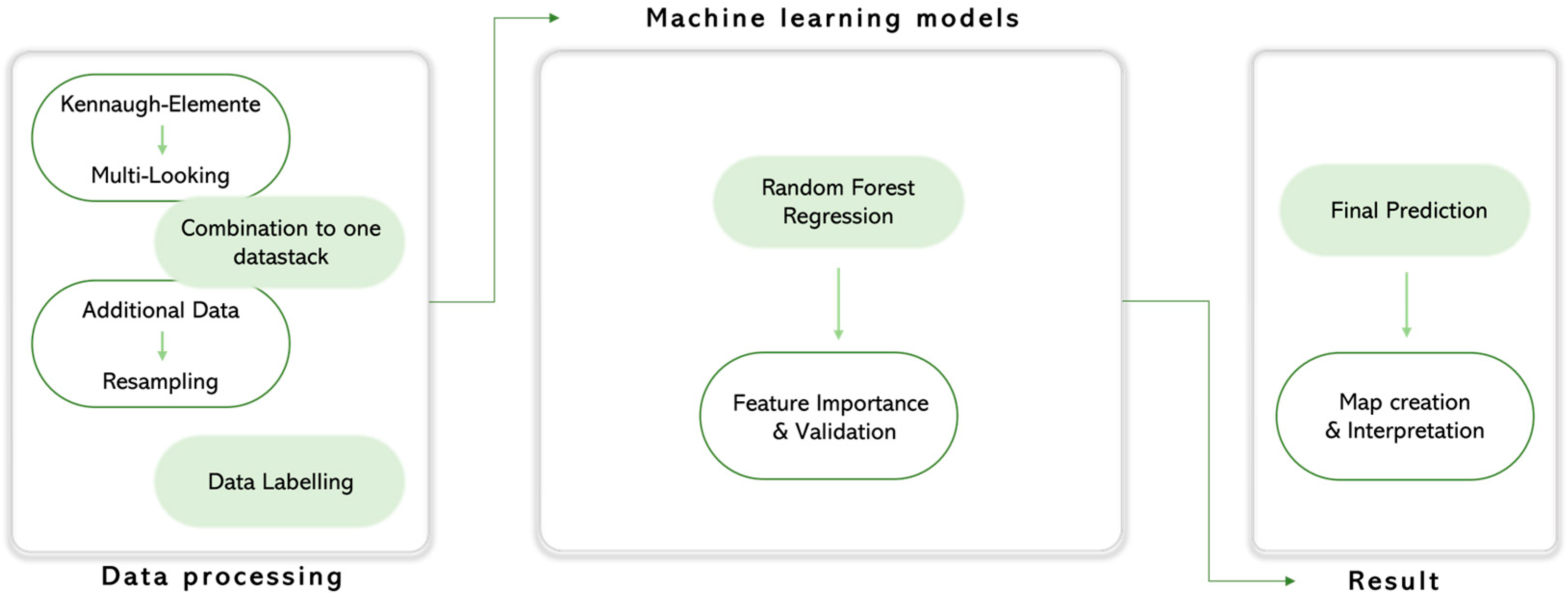
Considering the strong impact of drought on forest ecosystems, hydrological data using the Topographic Wetness Index (TWI), and the predominant soil types were included in the analysis (bogs, gley and gneiss granite substrate). The TWI represents the relief-related soil moisture and is therefore a good indicator for taking soil hydrology into account, especially in hilly terrain such as the Bavarian Forest. Based on the digital terrain model and information on the water catchment area, the runoff behaviour can be determined, which is decisive for the soil moisture. The TWI is made available for free use as a WMS by the Julius Kühn Institute in collaboration with the Research Center for Agricultural Remote Sensing [50]. To enable integration with Sentinel-1, the WMS data was converted into a raster with a spatial resolution of 10 m using the Python packages OWSLib 0.24.1 and rasterio 1.3.6. The area was requested from the WMS, geotransformed by specifying the bounding box as well as the target pixel size and was subsequently saved as a georeferenced GeoTIFF. Interpolation or resampling is not necessary, as the spatial reference was ensured by comparing the raster structure with the Sentinel-1 data. Due to the varying water storage capacities of the various soil types, a soil map at a scale of 1:25,000, a WMS provided by the Bavarian State Ministry of the Environment [51], was integrated into the database. This dataset allows deduction of the exact soil type under the tree stands and thus their water storage capacities. In the Bavarian Forest, a distinction can be made between the following soil types in terms of water storage capacity: moors, gley and granite or gneiss substrate.

3. Methods

The methodology is divided into three sections: a preliminary trend analysis, the prediction of tree vitality due to bark beetle infestation using Random Forest (RF) regression models, and the methodologically consistent spatial transfer to the North Rhine-Westphalia region.

3.1. Trend Analysis

Using the Sentinel-1 time series, more precisely the Kennaugh elements of the single acquisitions, a trend analysis was carried out, which was divided between known deadwood areas and healthy forests. The primary goal was to determine whether there was a correlation between the SAR backscatter and the health state of the trees. Consequently, it can also be deduced from this whether the stress in the trees due to drought or bark beetle infestation is evident. Therefore, a linear regression was evaluated using the metrics R-squared (R2) and Root Mean Square Error (RMSE). Both methods were applied to the previously defined epochs (see Figure 2). A major advantage of using trend information in combination with SAR is a further noise reduction, and therefore, an increased stability of the results.

3.2. Vitality Prediction

Figure 3 shows the steps taken to create the vitality map of the spruce trees to detect the green attack stage of the bark beetle infestation. The normalised Kennaugh elements were combined with the soil classes and the TWI to form a data stack. Consequently, RF regression models were created together with the prepared training data. According to a literature review on the early detection of bark beetle attacks, RF is the most frequently used algorithm in this area [10]. These models are also characterised by their robustness against overfitting, the handling of non-linear correlations and their simplicity, which reduces the need for large training datasets. Additionally, no prior assumptions about the data distribution are necessary, and feature importance can be estimated directly [52,53]. Model comparisons also demonstrate that the RF is well-suited for identification of bark beetle infestation. For example, in a study in Croatia, RF achieved the highest kappa value after the artificial neural network [54]. Another study comparing RF, XGBoost, Multi-Layer Perceptron and U-Net found that U-Net is the most accurate, followed by RF. However, RF is better at delineating hotspots and does not lead to a higher number of false positives than U-Net or Multi-Layer Perceptron [55]. RF regression therefore offers a promising analytical approach for assessing forest health and, consequently, the likelihood of bark beetle infestation. Additionally, regression allows for a precise estimation of the degree of damage to the spruce stands. This quantification is crucial for detecting bark beetle infestation on the ground. The continuous output also means that no information is lost in intermediate states. In a final step, the regression result can also be quantified into different classes if desired.
The input stack, consisting of the Kennaugh elements, the TWI and the soil classes, was subdivided into five epochs, as shown in Figure 2, which in turn generated five models. These epochs represented temporally distinct snapshots of forest condition, enabling a dynamic labelling approach, where the same reference polygons could carry different labels across epochs depending on their distance in time from the recorded infestation (see Table 2). This structure enabled the model to learn early-warning indicators of vitality decline up to two years in advance of recorded mortality and the loss of vitality could also be directly linked to the labels. This is because the label ‘4’ indicated that the stand will die in 2 years, and accordingly, the label ‘3’ evinced that it will die in one year. This approach supported both early detection and retrospective monitoring of bark beetle impact over multiple years.
The training and validation of the models were carried out using the five rasters created based on the deadwood data. For this purpose, the labelled pixels were divided into 80% training data and 20% validation data. In this way, the model performance could be objectively evaluated using unseen validation data. The metrics R2 and RMSE were determined to assess the statement’s quality. In addition, the so-called Shapley Additive exPlanations (SHAP) values were calculated to provide a deeper understanding of how each feature contributes to a particular prediction. The SHAP values are an additive decomposition of the prediction, whereby each prediction is made up of an expected value and the sum of all SHAP values. A positive SHAP value indicates that the feature increases the prediction, whereas a negative value decreases it. The amount indicates the relative importance of the features. As a result, the SHAP values not only allow a statement to be made about the importance of the feature, but they can also be used to determine that, for example, low values of a feature influence the prediction in a negative direction and thus, the prediction value becomes smaller. The final results of the prediction were then used to create maps that showed the development of the tree vitality, which related to the infestation of the bark beetle. They then showed how many years the trees are still healthy or at what point they became too weakened to effectively resist bark beetle attacks. To this end, the trained and validated models were applied to the entire Bavarian Forest National Park.

3.3. Regional Transfer

The RF regression methodology described was applied in the same way to the transfer region in North Rhine-Westphalia. The entire modelling workflow, including input feature construction, training data preparation, and regression setup, was retained without modification. Sentinel-1 image data from April to October in the years 2020 to 2023 were utilised, and the preprocessing steps followed the same procedure as in the Bavarian Forest National Park, including decomposition into Kennaugh elements, radiometric calibration, orthorectification, and multi-looking. Although the overall regression setup and label structure were retained, the TWI and soil type information were intentionally excluded in the transfer region to evaluate the Sentinel-1 Kennaugh elements as stand-alone predictors. This allowed for testing the model’s transferability without relying on auxiliary information (e.g., topographic), and helped to assess whether radar backscatter features, particularly K0, which represented total intensity, were sufficient for estimating forest vitality.
For each of the five-time steps considered (E1 to E5), the distributions of the predicted vitality classes were presented as a histogram. This enables the examination of whether the frequencies of the condition classes followed a plausible trajectory of ecological development over time. For example, an increasing proportion of stressed or dead stands in later epochs was an indication of consistent temporal modelling of the loss of vitality. To directly compare model predictions with available forest vitality loss data in North Rhine-Westphalia, the median predicted class values were calculated for each reference class. The external reference consists of eight damage categories ranging from “no change” to “total loss.” These were mapped to the internal five-class vitality scale (e.g., “total loss” and “severe damage” → class 1; “moderate decline” → class 3; “no change” → class 5). Median prediction trends were plotted across all epochs (E1–E5), separately for the reference years 2023 and 2024. This analysis enabled the evaluation of how the model responded to increasing severity in external labels helping to verify whether the predicted degradation aligned with real-world observations. Together, these methods ensured that the regression model not only performed well within each time step but also maintained temporal and ecological validity when applied to a new geographic context.

4. Results

4.1. Trend Analysis

Figure 4 illustrates the seasonal backscatter trends in K0 for both healthy forest and deadwood areas from April 2020 to October 2023. In healthy forest areas, K0 follows a seasonal cycle: it increases from spring through the summer months and declines in autumn and winter. This pattern aligns with vegetation growth cycles, likely reflecting increased density and moisture content during the growing season. The backscatter values for the healthy forest areas range from approximately −9.2 dB to −7.1 dB, with peak values typically occurring in mid-summer before declining towards the end of the growing season. This cyclical behaviour, maintained on a seasonal basis, persists throughout the study period.
A similar seasonal pattern is initially observed in areas that later transition to deadwood. Before dieback, these transitioning areas exhibit a pattern similar to that of healthy forests, although their backscatter values are generally lower, in a range of approximately −11.0 dB and −8.2 dB, about one decibel below those of fully healthy areas. A notable shift in the regression slope becomes visible around the time these areas were officially recorded as deadwood, marking the onset of significant structural degradation. For areas classified as deadwood in 2022, the seasonal trend flattens after dieback, with the regression slope approaching zero, indicating minimal seasonal variation. However, beginning in June 2022, a deviation from this flat trend appears: instead of the expected summer decline, a brief increase is observed, followed by a renewed drop starting in April. This negative slope continues until the end of the time series in October 2023 (see Figure 4), suggesting a stabilised, yet degraded condition.
The same applies to the change year 2020. However, in 2021, the regression for these transitioning areas drops sharply. In the years following the forest dieback, the regression again resembles the original seasonal pattern, characterised by a rising and falling trend.

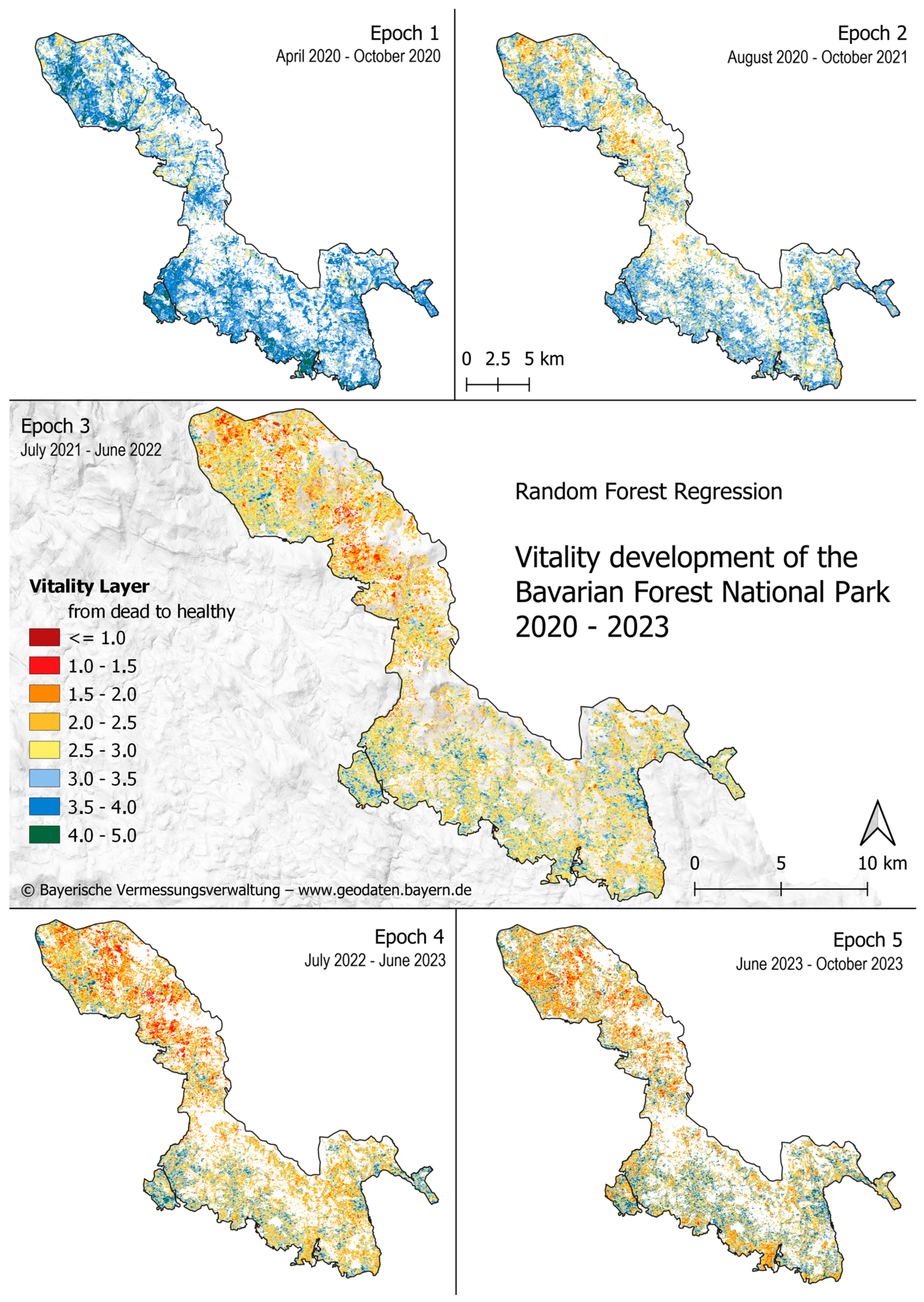
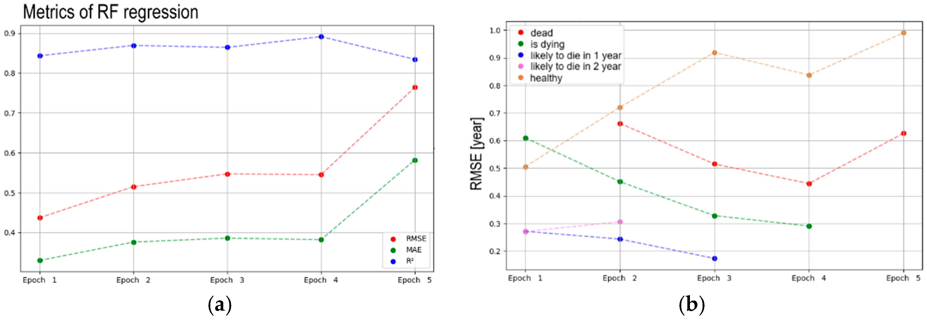
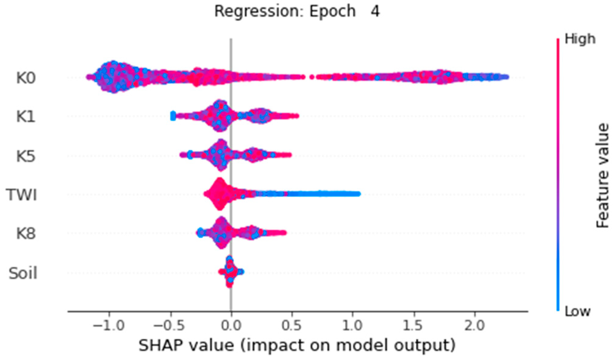
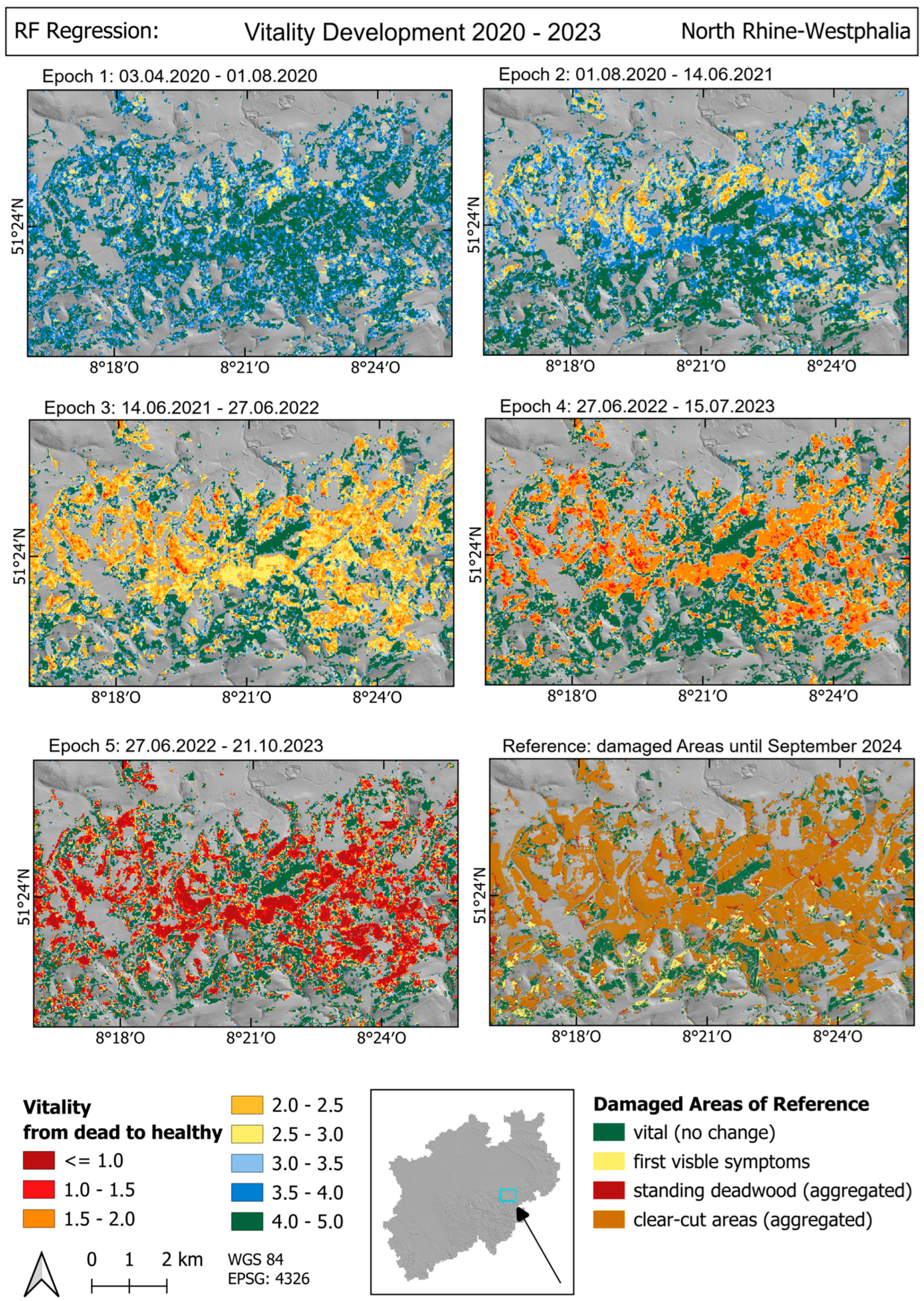
4.2. Vitality Prediction

The regression model applied to the forest vitality status, as shown in Figure 5, illustrates spatial and temporal variations in vitality levels from 2020 to 2023 in the Bavarian Forest National Park, including the timing of spruce stand mortality. Figure 6 is a selected close-up of the result applied to a test area, where the reference polygons were not used to train the model.
This approach allows for an independent assessment of the model’s predictive capability in regions outside the training data. The consistent vitality patterns observed in the transfer area indicate the model’s reliability and applicability to other forested landscapes. The displayed sequence of panels (see Figure 5) provides an annual view of changes in forest vitality conditions across the study areas. In the panel of Epoch 1, the central and northeastern sections predominantly show regions with low vitality. These areas, showing signs of stress and potential dieback, reflect reduced vitality early in the time series. In Epoch 2, these regions continued to exhibit low vitality, indicating a lack of significant recovery. A significant number of pixels in these zones transition to deadwood. In Epoch 3, the model shows an expansion of low vitality areas into the southern part of the area. These changes represent an increased distribution of stressed and dying spruce forests, as low vitality extends beyond the initial zones of dieback. Throughout all years, one area in the north-west consistently displays high vitality with no signs of degradation or deadwood. The panel of Epoch 4 continues to display large areas of low variability in the central and northeastern sections, where many regions likely reached the deadwood status. However, small patches of a relatively higher vitality begin to appear within previously orange zones. Within the Epoch 5, the overall pattern remains similar to Epoch 4, with extensive stressed and dying areas particularly in the northeastern region. Likewise, a further noticeable increase in vitality is observed in previously stressed areas, notably in the southern part of the map.
The R2 metric in Figure 7a, shown in blue, ranges from 0.83 to 0.89, indicating consistently strong model performance across the entire time series. The measures MAE and RMSE, which reflect the deviations between the predicted and actual values in the time unit of years, further confirm the model’s predictive accuracy. The best results achieved are 0.32 years for MAE and 0.43 years for RMSE. This means the model estimates the remaining healthy lifespan of spruce trees with an uncertainty of less than half a year. The weakest performance is observed in Epoch 5, where R2 drops to 0.83, while MAE and RMSE increase to 0.58 and 0.76 years, respectively. Therefore, it can be concluded that individual pixels were assigned incorrect vitality classes, resulting in a prediction error of up to three-quarters of a year in estimated tree mortality timing.
The SHAP values for Epoch 4, shown in Figure 8, offer the clearest insights into feature importance and the influence of individual variables on the RF regression model’s predictions across all epochs.
In Epoch 4, K0 (total intensity) stands out as the most influential feature, exhibiting the widest range of SHAP values across the dataset. K0 shows both positive and negative SHAP values, indicating that its variation contributes to predictions of both healthy and degraded conditions. The second most important feature is K1 (logarithmic intensity ratio between VV and VH). The SHAP values for K1 are more tightly clustered than those for K0, with a mixture of positive and negative values, suggesting its role in distinguishing varying levels of forest vitality, albeit with slightly lower influence. K5 and K8, both representing phase differences, follow as the next most influential features. They display moderate SHAP values, with K5 slightly more influential than K8. The SHAP distributions for these features are narrower compared to K0 and K1, indicating a more limited, yet notable, impact on prediction outcomes.
TWI and soil classifications appear at the lower end of the feature importance ranking for Epoch 4. TWI shows low but predominantly positive SHAP values, indicating a smaller but generally favourable influence on predictions. In contrast, soil classifications show a more varied distribution, with both positive and negative SHAP values, but with limited overall impact.
Across all epochs, K0 consistently ranks as the most important feature, followed by K1, confirming the dominance of backscatter intensity and its polarisation-based variation in predicting forest vitality. Beyond feature ranking, the directionality of K0’s SHAP values reveals additional insights: lower K0 values tend to reduce the predicted vitality score, whereas higher values increase it. This pattern is not observed for the other Kennaugh elements, emphasising the potential of the total intensity.

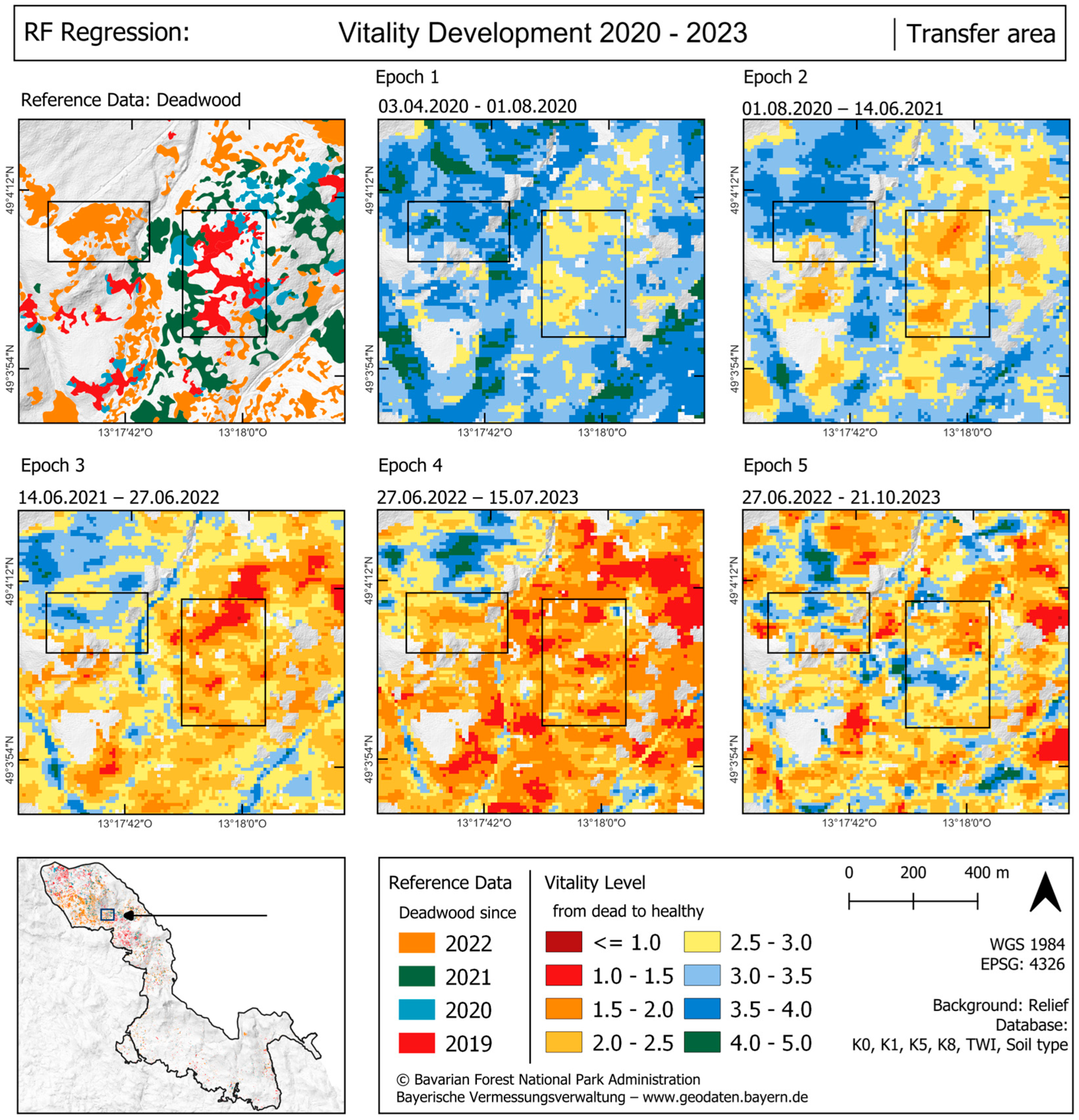
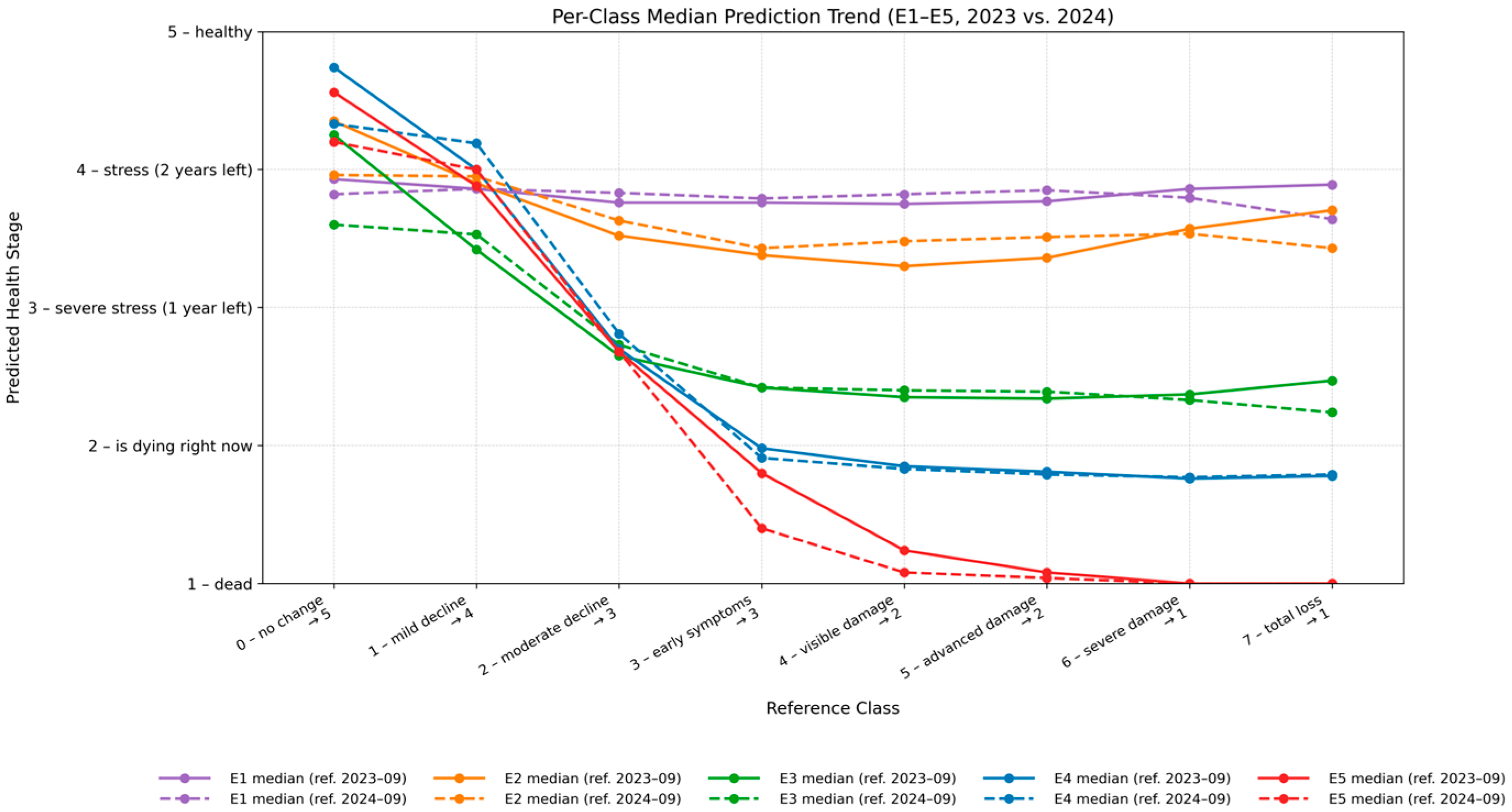
4.3. Regional Transfer

Similarly to the findings in the Bavarian Forest National Park, the predictions for North Rhine-Westphalia indicate a progressive decline in spruce stand vitality over time. This is illustrated in the individual panels by the transition from green or blue pixels to orange or red colouring in Figure 9, despite these areas not being used for training or validation. The reference data in the last panel show cleared forest patches in 2024. This pattern is already slightly apparent in Epoch 1 and becomes very clear in the following Epoch 2. A visual comparison of healthy spruce areas further confirms the model’s predictive accuracy.
To assess temporal consistency in the transfer region, cumulative distribution analysis was performed on the predicted vitality values for each epoch. Figure 10 shows the cumulative distribution functions (CDFs) of the regression outputs across all five epochs (E1 to E5). The predicted values are aligned with the continuous vitality scale ranging from 1.0 (dead) to 5.0 (healthy), with dashed vertical lines indicating the class thresholds used in the label definition. The distributions show a clear temporal gradient: earlier epochs (e.g., E1 and E2) exhibit higher vitality predictions concentrated toward the healthy end of the scale, while later epochs (e.g., E4 and E5) shift progressively toward lower predicted values. This confirms the validity of the dynamic labels, which were assigned based on the time since the recorded mortality. The model successfully distinguishes between older and more recent mortality signals, demonstrating its ability to generalise temporal vitality loss patterns. The smooth transitions and rising cumulative probabilities for low vitality scores in later epochs reflect the expected progression of bark beetle infestation, highlighting the model’s effectiveness and the robustness of the epoch-based labelling approach.
To evaluate the alignment of the model predictions with external reference data in the transfer region [49], a per-class median trend analysis was conducted. The available reference data in North Rhine-Westphalia from 2023 and 2024 includes eight classes describing forest vitality loss, ranging from “no change” to “total loss”. These were mapped onto the internal regression scale from 1 (dead) to 5 (healthy). Figure 11 shows the median predicted vitality scores per reference class for each epoch (E1–E5), plotted separately for 2023 and 2024. The results reveal a consistent downward trend in predicted vitality with increasing severity of the reference classes. Forest areas labelled as “no change” or “mild decline” are associated with higher predicted health scores, while “advanced damage” or “total loss” correspond to low vitality predictions. Notably, the later epochs (E4 and E5) exhibit steeper declines in predicted health, reflecting their temporal proximity to the reference year. The clear separation of curves across epochs and the monotonic structure of the trend support the model’s capacity to reflect real degradation gradients, further reinforcing the model’s adaptability across regions.

5. Discussion

5.1. Trend Analysis

The trend analysis demonstrates that the progression from healthy or stressed forests to dieback stages can be effectively monitored through changes in the Kennaugh elements of Sentinel-1 time series. This includes capturing the transition from the initial, often visually undetectable green attack phase to the subsequent red attack stage. As a key component of the Kennaugh decomposition, K0 represents the total backscatter intensity by combining VV and VH polarisation, capturing variations in both vegetation density and moisture content. This unique capability enables K0 to capture both seasonal variations and long-term trends in forest health linked to stress and mortality. The use of the segmented regression in this analysis provides further insight into seasonal patterns and transition points, allowing for a more detailed understanding of how backscatter values evolve (see Figure 4). Calculating segmented regression for individual epochs reveals transition points between seasonal phases, reflecting phenological changes in the forest canopy.
For example, during spring and early summer, healthy forest areas show a clear seasonal pattern. K0 values increase during the growing season, reflecting the phenological development of spruce trees through enhanced photosynthesis, moisture uptake, and tissue growth. However, the K0 intensity values start to decline during late summer, likely due to reduced water availability during this period. This seasonal reduction reflects the trees’ physiological response aimed at conserving water and reducing metabolic activity, a trend observable in the Sentinel-1 data. Studies such as those by Rüetschi et al. (2018) similarly report that backscatter from spruce trees in both VV and VH polarisation is lower in winter and higher during the growing season due to variations in moisture content and vegetation density [56]. This pattern contrasts with that of deciduous trees, which show increased backscatter following leaf fall in autumn due to structural changes in the canopy [56].
In contrast, areas documented as deadwood or exhibiting signs of advanced stress consistently display low K0 values throughout the year, with minimal seasonal variation. The flat trend in K0 values for deadwood areas indicates the absence of active growth and reduced moisture levels, both of which are typical indicators of degraded vegetation. This difference in K0 trends between healthy and deadwood areas highlights its effectiveness in distinguishing between actively growing and degraded vegetation.
The trend analysis further demonstrates a gradual decline in areas transitioning from healthy to stressed and eventually to dead trees. This progressive reduction in backscatter suggests a shift from high vitality to stress-induced degradation, characterised by a decrease in needle water content and, in a final step, canopy defoliation. These patterns are critical for the early detection of forest stress, during the green attack stage triggered by bark beetles, as declining K0 values may indicate the onset of degradation, before visible dieback symptoms appear in optical imagery.
In areas transitioning to deadwood, K0 values are consistently at least one decibel lower than in healthy forests. This shows that the overall intensity can reflect the changed structure of the forest. The reduced values indicate a lower water content and, thus, reduced vitality. These findings are consistent with those by Pirotti et al. (2023), who demonstrated that Sentinel-1 C-band backscatter, particularly in VH polarisation, is sensitive to canopy moisture, with drier conditions leading to reduced VH returns [57]. While their study focused on Mediterranean forests, the reported sensitivity of radar backscatter to moisture dynamics underlines the suitability of K0 for monitoring stress-induced decline in coniferous forest canopies. Early identification of stress-prone areas is crucial for proactive forest management, allowing for timely interventions to prevent further damage.

5.2. Vitality Prediction

The RF regression model performs very well in predicting forest vitality and mortality, as confirmed by both visual inspection and quantitative metrics (as shown in Figure 7: R2 between 0.83 and 0.89 and RMSE between 0.43 and 0.76 years). Before delving into the detailed metrics, two notable anomalies observed in the results in Figure 6 and Figure 7 should be addressed.
In some areas, the model indicates an implausible transition from “dead” to “stressed”, which may be attributed to mixed pixels containing both coniferous and deciduous trees. Deciduous trees, as observed by Rüetschi et al. (2018), exhibit seasonal backscatter patterns different from those of conifers, with greater variability in backscatter values due to phenological differences [56]. These differences likely interfere with the model’s predictions, resulting in misclassifications. Furthermore, signs of recovery in the spruce stands become apparent in the final Epoch 5. This apparent recovery process depends fundamentally on the ecosystem’s resilience—its capacity to absorb disturbances and gradually restore its original structural and functional attributes [58]. External factors such as climatic conditions and soil quality are also critical drivers. In particular, increased light availability following canopy loss, combined with sufficient water and nutrient supply, may have facilitated the rapid establishment of fast-growing understory species, like raspberry (‘Rubus idaeus’), feather reed grass (‘Calamagrostis arundinacea’), common dandelion (‘Taraxacum officinale’) as well as herbaceous plants [59]. These early successional species eventually dominate the backscatter signal. As a result, areas previously classified as deadwood may be misinterpreted by the model as areas of increasing vitality. Moreover, persistent precipitation in the preceding year may have further accelerated vegetative regrowth while simultaneously modifying the dielectric properties of the surface, thereby altering the SAR signal.
When interpreting this regeneration process, it is important to consider the model’s low performance in Epoch 5, which can be attributed to boundary effects caused by the inherent limitations of data at the edges of the time series. From a statistical perspective, it is therefore expected that marginal areas—such as the final time points in the analysed period—are modelled less precisely due to the reduced availability of surrounding data. This is explained by both truncated distribution effects and by the limited data availability, as future observations are missing [60]. The class-specific accuracies reveal that the “healthy” class is particularly challenging for prediction. This is because the value of the RMSE is always above 0.5 years and almost reaches 1.0 year in Epoch 5. It can be assumed that the model is more aligned with the stressed pixels, as the sum of the labels for the vitality levels “severe stress” (likely to die in 1 year) and “stress” (likely to die in 2 years) exceeds the amount of training data for the vital class. The fact that the model does not correctly decipher the variance in the vital forest class can be ruled out due to the similar R2 values of dead and intact spruce forests in the trend analysis. The model provides the best assignment for the class labelled as “severe stress” (label 3), followed by “stress” (label 4). In general, there is a tendency for the prediction error to increase in Epoch 5. Considering the availability of the training data, this is plausible, as the model was only trained on data differentiating between “deadwood” and “healthy”. Otherwise, the overall quality of the model remains relatively stable throughout the time series, although individual vitality levels fluctuate; all classes except the healthy one follow the same trend.
When interpreting the results, it is important to consider the temporal uncertainty of the reference data, since deadwood polygons are mapped annually without specifying the exact timing of tree mortality or bark beetle infestation. In addition, the Nyquist-Shannon theorem on data collection states that the sampling frequency must be at least twice as high as the fastest change in the vitality of the forest to be recorded. To detect bark beetle infestation, at least two satellite images per month along with corresponding bi-monthly reference data are required. The available satellite data from Sentinel-1 with up to four images per month provide an optimal basis. However, corresponding reference data with similar temporal resolution are lacking. This is because the reference data indicate only the year in which the spruce stand will die, while the precise timing of the initial bark beetle attack within this year remains unclear. The proposed methodology offers several advantages and fundamentally differs from previous approaches. This is because only polarisation ratios of VV to VH, backscatter coefficients, or statistical values, such as the standard deviation, have been used, as in [28,31,35]. The success of deriving the vitality of the spruce trees from the Sentinel-1 scenes depends mainly on the Kennaugh elements. On the one hand, unlike Tanase et al. (2018), for example, no recordings are removed after a precipitation event and, above all, no change analysis is carried out between just two recording states [31]. Additionally, the Sentinel-1 images enable continuous monitoring, unaffected by the frequent cloud cover typical of the Bavarian Forest. This aspect is crucial for early detection of bark beetles and highlights the advantage of radar data over optical images. König et al. (2023) achieved 62% accuracy with Sentinel-1 and 93% with Sentinel-2, yet infestation were detected on average 200 days after the actual infestation, rendering timely intervention impossible [28]. In an attempt to extract the early infestation stage, Abdullah et al. (2019) achieved an accuracy of 67%, which is equally inadequate for effectively managing the bark beetle [27]. At this point, the added value of the results becomes evident, as the final map reveals how many years specific forest areas have remained healthy, are currently in decline, or have already died, with an uncertainty of significantly less than one year. Notably, the model’s ability to differentiate stress levels with a temporal delay of less than half a year is particularly noteworthy. The “severe stress” class (label ‘3’), indicating high mortality risk within the next year, is predicted with an accuracy of under 109 days. This early warning capability enables proactive and spatially targeted bark beetle management, allowing interventions to be implemented before widespread infestation occurs. Although the precise timing of the green attack phase is not explicitly recorded in the reference data, it can be assumed to fall within the transition between severe stress and observable degradation. The combined predictive performance of the “severe-stress” and “is dying” classes yields an average temporal accuracy of approximately 125 days, offering a sufficiently narrow window to support effective monitoring.
The SHAP analysis identifies K0 as the most influential feature in predicting forest vitality across all epochs. This aligns with K0’s theoretical role in capturing forest structure, density, and moisture content, as it combines VV and VH polarisation components. High K0 values indicate increased water content therefore also chlorophyll content, resulting in higher backscatter values and healthier forest signals [56,57]. In contrast, low K0 values are associated with stressed or dead areas where backscatter intensity drops due to a reduction in canopy density and moisture. This dual relationship highlights K0’s robustness as a key indicator of vitality.
K1 ranks second in importance, capturing intensity differences between VV and VH, and thus providing structural detail about the canopy. This characteristic allows K1 to identify horizontal and vertical elements in the canopy, such as branches and crowns, which may indicate early signs of structural degradation and is crucial for distinguishing between healthy and degraded states. In the context of bark beetle infestation, changes in needle structure, initially due to reduced water content and, in more advanced stages, through needle thinning or loss, are captured by K1.
Although Kennaugh elements K5 and K8, which reflect phase difference and depolarisation, were initially expected to play a minimal role in vegetation studies, their moderate importance in the SHAP analysis suggests a potential to characterise forest degradation. These phase differences may capture coherence in the canopy structure that correlates with forest vitality. While traditionally used for deterministic targets, the relevance of K5 may indicate a sensitivity to structural disturbances in the canopy, such as those caused by stress or early dieback. Further investigation, potentially using causal analysis as recommended by Yu et al. (2020) [61], could provide additional insights into the specific contribution of phase information to vegetation monitoring.
TWI and soil classifications provide valuable ecological context to the model’s predictions by representing variations in soil moisture and drainage, which critically affect tree health. The SHAP analysis reveals that lower TWI values, indicating drier soils, generally are associated with higher vitality predictions, likely due to spruce trees’ adaptation to well-drained soils. Under these conditions, they tend to develop “sinker roots” that grow vertically downward to access groundwater, thereby enhancing their resilience in drier areas. A similar observation supports this, showing that trees with sinker roots in permeable soils exhibit better drought resistance [62]. In contrast, higher TWI values correlate with lower vitality predictions. In waterlogged or poorly aerated soils, spruce trees frequently develop shallow root systems, making them more susceptible to irreversible dieback during subsequent dry periods, disrupting the tree’s nutrient supply.
Soil classifications complement TWI by inversely correlating with vitality predictions: soils near groundwater (low soil class values), which have a high water retention capacity, tend to support less vital forests, while distant, well-drained soils (characterised by high soil class values) with a low water retention capacity align with higher vitality. This pattern aligns with the physiological adaptations of spruce trees, which develop different rooting strategies in response to varying soil moisture availability.
Although Epoch 4 serves as a representative example, notable anomalies also appear in other epochs, revealing the complexity of forest vitality prediction under varying conditions. The resulting observations, for example, the correlation between higher TWI values and higher vitality in Epoch 1, point to the need for a meteorological context to interpret the SHAP values correctly. This is because short-term fluctuations in soil moisture and climate, such as variations in precipitation, can influence the model results. Such temporal irregularities highlight the importance of collecting frequent, high-resolution data to differentiate between short-term anomalies and long-term trends in forest vitality. The SHAP analysis confirms the importance of radar backscatter (K0, K1) and phase-related characteristics of the radar (K5, K8) as well as topographic and hydrological factors (TWI, soil classes) for characterising forest health. It also demonstrates the temporally dynamic nature of these relationships and emphasises that the prediction of forest vitality depends not solely on isolated data points, but on the interplay of structural, ecological, and environmental factors.

5.3. Regional Transfer

The application of the vitality prediction model to North Rhine-Westphalia serves as a critical test for the methodological robustness and transferability of the Sentinel-1-based regression approach developed for the Bavarian Forest National Park. While earlier research often cautions against direct spatial transfers due to variation in topography, land use, or data availability [63,64,65], this study preserves model consistency by retraining the same RF regression structure with locally adapted labels, yet without modifying the core architecture, label logic, or EO feature processing.
A central aspect of this transfer was the deliberate exclusion of auxiliary contextual layers, such as the TWI, to evaluate the predictive performance of radar-based features alone. This design decision was based on our prior SHAP analysis and trend assessments in the Bavarian Forest, which consistently identified the Kennaugh element K0 as the most influential feature for vitality prediction. This strengthens the case for operational scalability, as radar-only approaches could be applied in regions lacking ancillary environmental data.
The importance of K0 to identify subtle pre-mortality phases becomes particularly evident when examining the predictions for North Rhine-Westphalia. As shown in the CDFs in Figure 10, vitality predictions consistently decline from epoch E1 to E5. This steady degradation trend supports the validity of the epoch-based dynamic labelling system and highlights the model’s capacity to identify early stress purely from radar-derived signals. Even in the absence of topographic or soil-related predictors, the model accurately captures temporally structured degradation patterns that exhibit strong ecological plausibility.
Further validation is provided by the per-class median trend analysis (Figure 11), where median vitality predictions show strong correspondence with external reference damage classes from 2023 and 2024. In particular, classes such as “visible damage” or “severe damage” align closely with predicted vitality values between 1.0 and 2.0. Importantly, these medians decline across successive epochs, reflecting the model’s temporal sensitivity and its external validity. These results confirm that the regression model can distinguish vitality gradients and associate them with real-world degradation stages, even in ecologically different forest regions.
Moreover, these findings reaffirm the ecological interpretability of K0: high values indicate intact forest conditions with full canopy moisture and structure, while lower values capture early warning signals linked to physiological stress or bark beetle impact. As shown in earlier seasonal trend analysis in the main study area, K0 also reflects seasonal dynamics, peaking in spring and declining during late summer. In contrast, stressed and dead areas show flattened K0 profiles, lacking these seasonal signatures.
The consistent trends observed in both cumulative and median-based validations underscore the success of the regional transfer to North Rhine-Westphalia and highlight the robustness and generalisability of the proposed methodology, particularly the EO data preparation pipeline and dynamic labelling approach. The predictive strength of Sentinel-1 backscatter intensity, especially the K0 element, demonstrates that a simplified, radar-based input stack is sufficient for consistent forest vitality monitoring. While ancillary data layers such as TWI and soil water capacity can enrich the understanding of belowground conditions; however, their omission does not critically compromise the model’s ability to detect forest degradation. This makes the approach highly suitable for rapid deployment in data-scarce regions and for scalable, operational forest monitoring across diverse ecosystems.

6. Conclusions

This study provides the first clear evidence of a significant correlation between the SAR signal over time and bark beetle infestation in spruce stands, allowing for the prediction of potentially affected areas before symptoms appear in optical imagery. The strength of our approach lies in the systematic preprocessing of SAR data into analysis-ready formats and the integration of dynamic vitality labels derived from comprehensive deadwood inventories, resulting in a temporally labelled data cube well-suited for machine learning models to capture degradation pathways. Our findings reveal that healthy and stressed spruce forests exhibit distinctive temporal signatures in the total intensity K0 of Sentinel-1 data, enabling a random forest regression model to predict forest vitality up to three years in advance, with a temporal uncertainty of approximately six months, primarily attributable to the sparsity of reference data. Successful transfer from the original study site in the Bavarian Forest National Park to forest areas in North Rhine-Westphalia, albeit via site-specific retraining, underscores the potential for broader application.
Although the absence of relevant, temporally dense reference data currently limits our ability to distinctly separate stressed from infested trees, the early detection of stressed trees, which are predisposed to infestation, provides a critical predictive tool for proactive forest management. This temporal uncertainty is one crucial point, to be addressed in follow-on studies, which can only be solved by regular reference data acquisition over large areas, a costly process. From a methodological point of view, the scalability remains an open issue. The presented results are based on regular repeat pass acquisitions by Sentinel-1. With a view to regional and national applications, where the input images vary in time, aspect and incidence angle, an extension of the Multi-SAR framework to a consistent temporal frame becomes necessary. In this context, the multi-temporal fusion of satellite data using hypercomplex bases may play a significant role [66]. Another up-to-date machine learning regressor might replace the currently used random forest regression to further enhance performance. Considering the required improvements identified above, the presented methodology can be easily implemented on a cloud-based platform.
Beyond the specific case of bark beetle infestation, the approach demonstrates how temporal patterns in SAR data can serve as early indicators of changes in forest vitality. This opens up new possibilities for detecting a broader range of biotic stressors, including fungal diseases or other insect outbreaks. By combining Sentinel-1’s cloud-resilient, high-frequency acquisitions with a scalable analytical framework, the method provides a dependable, operational tool for modern forest management, supporting timely responses to various disturbance scenarios.

Author Contributions

Conceptualization and methodology, A.S. and S.H.; software, C.H. and S.H. and A.W.; formal analysis and investigation, C.H. and S.H.; resources, A.S. and A.W.; writing—original draft preparation, C.H., S.H. and A.S.; writing—review and editing, all authors; visualisation, C.H.; supervision, A.S. and A.W., data curation, M.H. All authors have read and agreed to the published version of the manuscript.

Funding

This research received no external funding.

Data Availability Statement

The Sentinel-1 data is freely accessible as part of the Copernicus program via the Copernicus Data Space Ecosystem. Data processing from Sentinel-1 SLC products to Kennaugh elements can be carried out using the SNAP graph published as part of the Wald5Dplus benchmark dataset on Zenodo (https://doi.org/10.5281/zenodo.10848838). The deadwood data in the Bavarian Forest National Park were provided by the Bavarian National Park under the Bohemian Forest Datapool Initiative [39].

Acknowledgments

The authors like to thank the European Space Agency (ESA) for the provision of Sentinel-1 data ©ESA, 2020–2023 and the Copernicus Digital Elevation model. Special thanks go to the Bohemian Forest Datapool Initiative [39] for sharing the deadwood data. Furthermore, open access information products provided by the Julius Kühn Institute, the Research Center for Agricultural Remote Sensing, the Bavarian State Ministry of the Environment, the North Rhine-Westphalia State Forest and Wood Management and the Agency for Digitisation, High-Speed Internet and Surveying are used in this study.

Conflicts of Interest

The authors declare no conflicts of interest.

References

  1. Aquino, C.; Balzarolo, M.; Chiriacò, M.V.; Santini, M. Advancing Forest Cover and Forest Cover Change Mapping for SDG 15: A Novel Approach Using Copernicus Data Products. In Proceedings of the Copernicus Meetings, EGU24-15509, Vienna, Austria, 14–19 April 2024. [Google Scholar] [CrossRef]
  2. Espíndola, R.P.; Ebecken, N.F.F. Advances in remote sensing for sustainable forest management: Monitoring and protecting natural resources. Rev. Caribeña Cienc. Soc. 2023, 12, 1605–1617. [Google Scholar] [CrossRef]
  3. Huete, A.R. Vegetation Indices, Remote Sensing and Forest Monitoring. Geogr. Compass 2012, 6, 513–532. [Google Scholar] [CrossRef]
  4. Massey, R.; Berner, L.T.; Foster, A.C.; Goetz, S.J.; Vepakomma, U. Remote Sensing Tools for Monitoring Forests and Tracking Their Dynamics. In Boreal Forests in the Face of Climate Change: Sustainable Management; Girona, M.M., Morin, H., Gauthier, S., Bergeron, Y., Eds.; Springer International Publishing: Cham, Switzerland, 2023; pp. 637–655. [Google Scholar] [CrossRef]
  5. Økland, B.; Flø, D.; Schroeder, M.; Zach, P.; Cocos, D.; Martikainen, P.; Siitonen, J.; Mandelshtam, M.Y.; Musolin, D.L.; Neuvonen, S.; et al. Range expansion of the small spruce bark beetle Ips amitinus: A newcomer in northern Europe. Agric. For. Entomol. 2019, 21, 286–298. [Google Scholar] [CrossRef]
  6. Biedermann, P.H.; Müller, J.; Grégoire, J.-C.; Gruppe, A.; Hagge, J.; Hammerbacher, A.; Hofstetter, R.W.; Kandasamy, D.; Kolarik, M.; Kostovcik, M.; et al. Bark Beetle Population Dynamics in the Anthropocene: Challenges and Solutions. Trends Ecol. Evol. 2019, 34, 914–924. [Google Scholar] [CrossRef] [PubMed]
  7. Nationalparkverwaltung Bayerischer Wald. Habitats in the Bavarian Forest National Park. Available online: https://www.nationalpark-bayerischer-wald.bayern.de/english/nature/habitats/index.htm (accessed on 27 September 2024).
  8. Senf, C.; Buras, A.; Zang, C.S.; Rammig, A.; Seidl, R. Excess forest mortality is consistently linked to drought across Europe. Nat. Commun. 2020, 11, 6200. [Google Scholar] [CrossRef]
  9. Singh, V.V.; Naseer, A.; Mogilicherla, K.; Trubin, A.; Zabihi, K.; Roy, A.; Jakuš, R.; Erbilgin, N. Understanding bark beetle outbreaks: Exploring the impact of changing temperature regimes, droughts, forest structure, and prospects for future forest pest management. Rev. Environ. Sci. Biotechnol. 2024, 23, 257–290. [Google Scholar] [CrossRef]
  10. Marvasti-Zadeh, S.M.; Goodsman, D.; Ray, N.; Erbilgin, N. Early Detection of Bark Beetle Attack Using Remote Sensing and Machine Learning: A Review. ACM Comput. Surv. 2023, 56, 1–40. [Google Scholar] [CrossRef]
  11. Fahse, L.; Heurich, M. Simulation and analysis of outbreaks of bark beetle infestations and their management at the stand level. Ecol. Model. 2011, 222, 1833–1846. [Google Scholar] [CrossRef]
  12. Kautz, M.; Feurer, J.; Adler, P. Early detection of bark beetle (Ips typographus) infestations by remote sensing—A critical review of recent research. For. Ecol. Manag. 2024, 556, 121595. [Google Scholar] [CrossRef]
  13. Ghorbanian, M.; Karimi-Malati, A.; Jalaeian, M.; Sangani, M.F. Maximum entropy modelling to predict the impact of abiotic variables on the potential distribution of Orthotomicus erosus (Wollaston) (Coleoptera, Curculionidae, Scolytinae). J. Insect Biodivers. Syst. 2023, 9, 711–725. [Google Scholar] [CrossRef]
  14. Lissovsky, A.A.; Dudov, S.V. Species-Distribution Modeling: Advantages and Limitations of Its Application. 2. MaxEnt. Biol. Bull. Rev. 2021, 11, 265–275. [Google Scholar] [CrossRef]
  15. Öhrn, P.; Långström, B.; Lindelöw, Å.; Björklund, N. Seasonal flight patterns of Ips typographus in southern S weden and thermal sums required for emergence. Agric. For. Entomol. 2014, 16, 147–157. [Google Scholar] [CrossRef]
  16. Heurich, M.; Beudert, B.; Rall, H.; Křenová, Z. National Parks as Model Regions for Interdisciplinary Long-Term Ecological Research: The Bavarian Forest and Šumavá National Parks Underway to Transboundary Ecosystem Research. In Long-Term Ecological Research; Müller, F., Baessler, C., Schubert, H., Klotz, S., Eds.; Springer: Dordrecht, The Netherlands, 2010; pp. 327–344. [Google Scholar] [CrossRef]
  17. Marini, L.; Lindelöw, Å.; Jönsson, A.M.; Wulff, S.; Schroeder, L.M. Population dynamics of the spruce bark beetle: A long-term study. Oikos 2013, 122, 1768–1776. [Google Scholar] [CrossRef]
  18. Jönsson, A.M.; Harding, S.; Bärring, L.; Ravn, H.P. Impact of climate change on the population dynamics of Ips typographus in southern Sweden. Agric. For. Meteorol. 2007, 146, 70–81. [Google Scholar] [CrossRef]
  19. Hollaus, M.; Vreugdenhil, M. Radar Satellite Imagery for Detecting Bark Beetle Outbreaks in Forests. Curr. For. Rep. 2019, 5, 240–250. [Google Scholar] [CrossRef]
  20. Huo, L.; Persson, H.J.; Lindberg, E. Early detection of forest stress from European spruce bark beetle attack, and a new vegetation index: Normalized distance red & SWIR (NDRS). Remote Sens. Environ. 2021, 255, 112240. [Google Scholar] [CrossRef]
  21. Abdullah, H.; Skidmore, A.K.; Darvishzadeh, R.; Heurich, M. Timing of red-edge and shortwave infrared reflectance critical for early stress detection induced by bark beetle (Ips typographus, L.) attack. Int. J. Appl. Earth Obs. Geoinf. 2019, 82, 101900. [Google Scholar] [CrossRef]
  22. Ali, A.M.; Abdullah, H.; Darvishzadeh, R.; Skidmore, A.K.; Heurich, M.; Roeoesli, C.; Paganini, M.; Heiden, U.; Marshall, D. Canopy chlorophyll content retrieved from time series remote sensing data as a proxy for detecting bark beetle infestation. Remote Sens. Appl. Soc. Environ. 2021, 22, 100524. [Google Scholar] [CrossRef]
  23. Pulliainen, J.; Hari, P.; Hallikainen, M.; Patrikainen, N.; Peramaki, M.; Kolari, P. Monitoring of soil moisture and vegetation water content variations in boreal forest from C-band SAR data. In Proceedings of the IGARSS 2004, 2004 IEEE International Geoscience and Remote Sensing Symposium, Anchorage, AK, USA, 20–24 September 2004; pp. 1013–1016. [Google Scholar] [CrossRef]
  24. Bernardino, P.N.; Oliveira, R.S.; Van Meerbeek, K.; Hirota, M.; Furtado, M.N.; A Sanches, I.; Somers, B. Estimating vegetation water content from Sentinel-1 C-band SAR data over savanna and grassland ecosystems. Environ. Res. Lett. 2024, 19, 034019. [Google Scholar] [CrossRef]
  25. Vreugdenhil, M.; Wagner, W.; Bauer-Marschallinger, B.; Pfeil, I.; Teubner, I.; Rüdiger, C.; Strauss, P. Sensitivity of Sentinel-1 Backscatter to Vegetation Dynamics: An Austrian Case Study. Remote Sens. 2018, 10, 1396. [Google Scholar] [CrossRef]
  26. Senf, C.; Seidl, R.; Hostert, P. Remote sensing of forest insect disturbances: Current state and future directions. Int. J. Appl. Earth Obs. Geoinf. 2017, 60, 49–60. [Google Scholar] [CrossRef]
  27. Abdullah, H.; Skidmore, A.K.; Darvishzadeh, R.; Heurich, M.; Pettorelli, N.; Disney, M. Sentinel-2 accurately maps green-attack stage of European spruce bark beetle (Ips typographus, L.) compared with Landsat-8. Remote Sens. Ecol. Conserv. 2018, 5, 87–106. [Google Scholar] [CrossRef]
  28. König, S.; Thonfeld, F.; Förster, M.; Dubovyk, O.; Heurich, M. Assessing Combinations of Landsat, Sentinel-2 and Sentinel-1 Time series for Detecting Bark Beetle Infestations. GISci. Remote Sens. 2023, 60, 2226515. [Google Scholar] [CrossRef]
  29. Bárta, V.; Lukeš, P.; Homolová, L. Early detection of bark beetle infestation in Norway spruce forests of Central Europe using Sentinel-2. Int. J. Appl. Earth Obs. Geoinf. 2021, 100, 102335. [Google Scholar] [CrossRef]
  30. Hesslerová, P.; Huryna, H.; Pokorný, J.; Procházka, J. The effect of forest disturbance on landscape temperature. Ecol. Eng. 2018, 120, 345–354. [Google Scholar] [CrossRef]
  31. Tanase, M.A.; Aponte, C.; Mermoz, S.; Bouvet, A.; Le Toan, T.; Heurich, M. Detection of windthrows and insect outbreaks by L-band SAR: A case study in the Bavarian Forest National Park. Remote Sens. Environ. 2018, 209, 700–711. [Google Scholar] [CrossRef]
  32. Schmitt, A.; Wendleder, A.; Hinz, S. The Kennaugh element framework for multi-scale, multi-polarized, multi-temporal and multi-frequency SAR image preparation. ISPRS J. Photogramm. Remote Sens. 2015, 102, 122–139. [Google Scholar] [CrossRef]
  33. Hoekman, D.H. Measurements of the backscatter and attenuation properties of forest stands at X-, C- and L-band. Remote Sens. Environ. 1987, 23, 397–416. [Google Scholar] [CrossRef]
  34. Konings, A.G.; Rao, K.; Steele-Dunne, S.C. Macro to micro: Microwave remote sensing of plant water content for physiology and ecology. New Phytol. 2019, 223, 1166–1172. [Google Scholar] [CrossRef] [PubMed]
  35. Kaiser, P.; Buddenbaum, H.; Nink, S.; Hill, J. Potential of Sentinel-1 Data for Spatially and Temporally High-Resolution Detection of Drought Affected Forest Stands. Forests 2022, 13, 2148. [Google Scholar] [CrossRef]
  36. Bae, S.; Müller, J.; Förster, B.; Hilmers, T.; Hochrein, S.; Jacobs, M.; Leroy, B.M.L.; Pretzsch, H.; Weisser, W.W.; Mitesser, O. Tracking the temporal dynamics of insect defoliation by high-resolution radar satellite data. Methods Ecol. Evol. 2021, 13, 121–132. [Google Scholar] [CrossRef]
  37. Nationalparkverwaltung Bayerischer Wald. Profile of Bavarian Forest National Park. Available online: https://www.nationalpark-bayerischer-wald.bayern.de/english/about_us/profile/index.htm (accessed on 27 September 2024).
  38. Seidl, R.; Müeller, J.; Hothorn, T.; Bässler, C.; Heurich, M.; Kautz, M. Small beetle, large-scale drivers: How regional and landscape factors affect outbreaks of the European spruce bark beetle. J. Appl. Ecol. 2016, 53, 530–540. [Google Scholar] [CrossRef]
  39. Latifi, H.; Holzwarth, S.; Skidmore, A.; Brůna, J.; Červenka, J.; Darvishzadeh, R.; Hais, M.; Heiden, U.; Homolová, L.; Krzystek, P.; et al. A laboratory for conceiving Essential Biodiversity Variables (EBVs)—The “Data pool initiative for the Bohemian Forest Ecosystem”. Methods Ecol. Evol. 2021, 12, 2073–2083. [Google Scholar] [CrossRef]
  40. Landesbetrieb Wald und Holz Nordrhein-Westfalen. Datenbestand des Landesbetriebes Wald und Holz NRW [Data from the State Forestry and Timber Agency of North Rhine-Westphalia]. 2024. Available online: https://www.wms.nrw.de/umwelt/waldNRW?SERVICE=WMS&REQUEST=GetCapabilities (accessed on 16 June 2025).
  41. Bertram, A.; Wendleder, A.; Schmitt, A.; Huber, M. Long-term Monitoring of water dynamics in the Sahel region using the Multi-SAR-System. In International Archives of the Photogrammetry, Remote Sensing and Spatial Information Sciences—ISPRS Archives; International Society for Photogrammetry and Remote Sensing (ISPRS), Publisher: Prague, Czech Republic, 2016; pp. 9–16. [Google Scholar] [CrossRef]
  42. Small, D. Flattening Gamma: Radiometric Terrain Correction for SAR Imagery. IEEE Trans. Geosci. Remote Sens. 2011, 49, 3081–3093. [Google Scholar] [CrossRef]
  43. Akhavan, Z.; Hasanlou, M.; Hosseini, M. A Comparison of Tree-based Regression Models for Soil Moisture Estimation using SAR Data. ISPRS Ann. Photogramm. Remote Sens. Spat. Inf. Sci. 2023, X-4/W1-202, 37–42. [Google Scholar] [CrossRef]
  44. Bai, X.; He, B.; Li, X.; Zeng, J.; Wang, X.; Wang, Z.; Zeng, Y.; Su, Z. First Assessment of Sentinel-1A Data for Surface Soil Moisture Estimations Using a Coupled Water Cloud Model and Advanced Integral Equation Model over the Tibetan Plateau. Remote Sens. 2017, 9, 714. [Google Scholar] [CrossRef]
  45. Le Hegarat-Mascle, S.; Zribi, M.; Alem, F.; Weisse, A.; Loumagne, C. Soil moisture estimation from ERS/SAR data: Toward an operational methodology. IEEE Trans. Geosci. Remote Sens. 2002, 40, 2647–2658. [Google Scholar] [CrossRef]
  46. Moreira, A.; Prats-Iraola, P.; Younis, M.; Krieger, G.; Hajnsek, I.; Papathanassiou, K.P. A tutorial on synthetic aperture radar. IEEE Geosci. Remote Sens. Mag. 2013, 1, 6–43. [Google Scholar] [CrossRef]
  47. Touzi, R. Target Scattering Decomposition in Terms of Roll-Invariant Target Parameters. IEEE Trans. Geosci. Remote Sens. 2007, 45, 73–84. [Google Scholar] [CrossRef]
  48. Landesbetrieb Wald und Holz Nordrhein-Westfalen. Vitalitätsabnahme und Kalamitätskarte Nadelwald NRW [Vitality Decline and Calamity Map of Coniferous Forests in North Rhine-Westphalia]. 2024. Available online: https://open.nrw/dataset/a0fab723-b852-4f8f-adf5-2723699149ff (accessed on 16 June 2025).
  49. Landesbetrieb Wald und Holz Nordrhein-Westfalen. Vitalitätsabnahme Nadelwald NRW [Decrease in vitality of coniferous forest in North Rhine-Westphalia]. 2024. Available online: https://www.opengeodata.nrw.de/produkte/umwelt_klima/wald_forst/fernerkundung/ (accessed on 16 June 2025).
  50. Julius Kühn-Institut. Topographischer Feuchteindex. Available online: https://wms.flf.julius-kuehn.de/cgi-bin/twi/qgis_mapserv.fcgi (accessed on 10 February 2024).
  51. Bayerisches Landesamt für Umwelt. Übersichtsbodenkarte 1:25.000. Available online: https://www.lfu.bayern.de/boden/karten_daten/uebk25/index.htm (accessed on 19 October 2024).
  52. Breiman, L. Random Forests. Mach. Learn. 2001, 45, 5–32. [Google Scholar] [CrossRef]
  53. Belgiu, M.; Drăguţ, L. Random forest in remote sensing: A review of applications and future directions. ISPRS J. Photogramm. Remote Sens. 2016, 114, 24–31. [Google Scholar] [CrossRef]
  54. Kranjčić, N.; Cetl, V.; Matijević, H.; Markovinović, D. Comparing Different Machine Learning Options to Map Bark Beetle Infestations in Croatia. Int. Arch. Photogramm. Remote Sens. Spat. Inf. Sci. 2023, XLVIII-4/W, 83–88. [Google Scholar] [CrossRef]
  55. Andresini, G.; Appice, A.; Ienco, D.; Malerba, D.; Recchia, V. Potential of Spectral-Spatial Analysis to Map Forest Tree Dieback Due to Bark Beetle Hotspots in Sentinel-2 Images. In Proceedings of the IGARSS 2024—2024 IEEE International Geoscience and Remote Sensing Symposium, Athens, Greece, 7–12 July 2024; pp. 5227–5230. [Google Scholar] [CrossRef]
  56. Rüetschi, M.; Schaepman, M.E.; Small, D. Using Multitemporal Sentinel-1 C-band Backscatter to Monitor Phenology and Classify Deciduous and Coniferous Forests in Northern Switzerland. Remote Sens. 2018, 10, 55. [Google Scholar] [CrossRef]
  57. Pirotti, F.; Adedipe, O.; Leblon, B. Sentinel-1 Response to Canopy Moisture in Mediterranean Forests before and after Fire Events. Remote Sens. 2023, 15, 823. [Google Scholar] [CrossRef]
  58. Drever, C.R.; Peterson, G.; Messier, C.; Bergeron, Y.; Flannigan, M. Can forest management based on natural disturbances maintain ecological resilience? Can. J. For. Res. 2006, 36, 2285–2299. [Google Scholar] [CrossRef]
  59. Matuszkiewicz, J.M.; Affek, A.N.; Zaniewski, P.; Kołaczkowska, E. Early response of understory vegetation to the mass dieback of Norway spruce in the European lowland temperate forest. For. Ecosyst. 2024, 11, 100177. [Google Scholar] [CrossRef]
  60. Loaiciga, H.A.; Michaelsen, J.; Hudak, P.F. Truncated Distributions in Hydrologic Analysis. JAWRA J. Am. Water Resour. Assoc. 1992, 28, 853–863. [Google Scholar] [CrossRef]
  61. Yu, K.; Guo, X.; Liu, L.; Li, J.; Wang, H.; Ling, Z.; Wu, X. Causality-based Feature Selection: Methods and Evaluations. ACM Comput. Surv. 2020, 53, 1–36. [Google Scholar] [CrossRef]
  62. Štofko, P.; Kodrík, M. Are there any differences in the root branch architecture of Norway spruce trees growing on two sites with different water regime? Folia For. Polonica. Ser. A Forestry 2009, 51, 181–184. [Google Scholar] [CrossRef]
  63. Jin, S.; Su, Y.; Gao, S.; Hu, T.; Liu, J.; Guo, Q. The Transferability of Random Forest in Canopy Height Estimation from Multi-Source Remote Sensing Data. Remote Sens. 2018, 10, 1183. [Google Scholar] [CrossRef]
  64. Hoppe, H.; Dietrich, P.; Marzahn, P.; Weiß, T.; Nitzsche, C.; von Lukas, U.F.; Wengerek, T.; Borg, E. Transferability of Machine Learning Models for Crop Classification in Remote Sensing Imagery Using a New Test Methodology: A Study on Phenological, Temporal, and Spatial Influences. Remote Sens. 2024, 16, 1493. [Google Scholar] [CrossRef]
  65. Qiu, C.; Li, H.; Guo, W.; Chen, X.; Yu, A.; Tong, X.; Schmitt, M. Transferring Transformer-Based Models for Cross-Area Building Extraction From Remote Sensing Images. IEEE J. Sel. Top. Appl. Earth Obs. Remote Sens. 2022, 15, 4104–4116. [Google Scholar] [CrossRef]
  66. Schmitt, A.; Wendleder, A.; Kleynmans, R.; Hell, M.; Roth, A.; Hinz, S. Multi-Source and Multi-Temporal Image Fusion on Hypercomplex Bases. Remote Sens. 2020, 12, 943. [Google Scholar] [CrossRef]
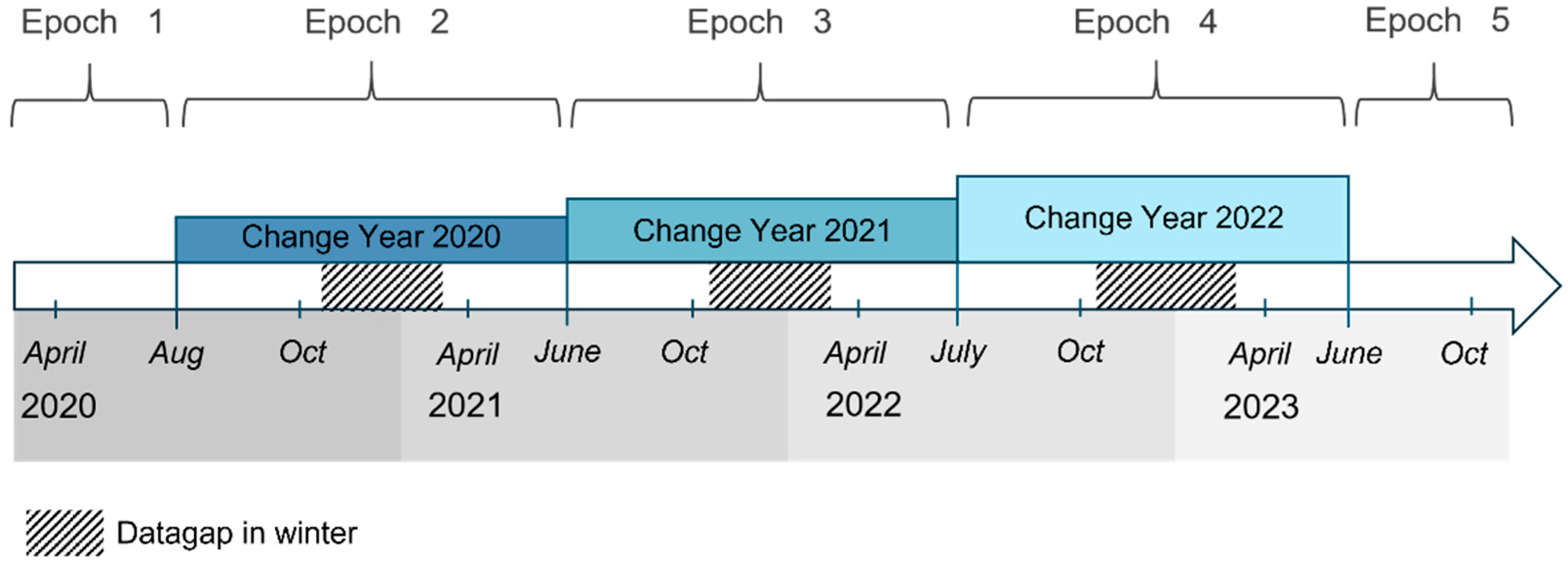
Figure 1. The map on the lleft side shows the training site Bavarian Forest National Park including the bark beetle infested areas [39], which are coloured according to the year of infestation. Blue indicates areas that were dead at the beginning of the survey in 1988, while the yellow colouring highlights current forest dieback. The right-hand side depicts the transfer area in North Rhine-Westphalia with the spruce stand in light blue and the damaged areas in red [40].
Forests 16 01272 g001
Figure 2. Categorisation of the satellite data into five epochs according to the change years recorded in the deadwood database of the Bavarian Forest National Park Administration [39]. As the bark beetle is only active in summer, winter acquisitions are not considered, reducing the amount of data to be processed.
Forests 16 01272 g002
Figure 3. Workflow for detection of bark beetle infestation and vitality development of forest using Sentinel-1 time series.
Forests 16 01272 g003
Figure 4. Linear regression (LR) for both healthy forest and deadwood areas: an alternating increasing and decreasing trend is visible; from the time of death onwards, the slope usually approaches zero. From April 2022, the availability of imagery diminished due to the failure of Sentinel-1B. The grey color indicates the unobserved period in winter. The regression equations displayed below the diagram are differentiated by between areas recorded as deadwood in 2022 and healthy spruce stands.
Forests 16 01272 g004
Figure 5. Prediction of vitality from increasingly stressed to dead for the Bavarian Forest National Park using RF regression: each panel represents a different epoch, with the colour coding of the vitality levels ranging from red (indicating low vitality–stressed, dying, or deadwood areas) to blue (high vitality) to green (healthy areas).
Forests 16 01272 g005
Figure 6. Prediction of vitality in an area not included in the training data using random forest regression: a clear decline in vitality is visible, aligning temporally with the reference data shown in the first panel. The two black frames are intended to help track the development of the reference polygons more easily.
Forests 16 01272 g006
Figure 7. High quality of the regression model is shown by: (a) the standard evaluation metrics R2, RMSE in units of years, and MAE; (b) and the class-specific RMSE, indicating that the “likely to die within 1 year” vitality class exhibits the highest predictive accuracy.
Forests 16 01272 g007
Figure 8. SHAP values of the incorporated features using Epoch 4 as an example: K0 has the highest influence on the prediction value. Low K0 values affect predictive outcomes in both positive and negative ways. Notably, for the TWI, lower values clearly increase the predictive value, i.e., topographically dryer areas are more prone to bark beetle infestation.
Forests 16 01272 g008
Figure 9. Predictions of vitality development in a transfer area using RF regression models, trained with data in North Rhine-Westphalia [48,49]. The bottom right panel presents the reference data provided by the state of North Rhine-Westphalia [49], where “clear-cut areas” correspond to formerly infested spruce stands prior to logging. Across the predictions of the five epochs, a progressive decline in vitality is evident in these areas, ranging from early stress symptoms (blue to yellow) to mortality progression (orange) and complete dieback (red).
Forests 16 01272 g009
Figure 10. Cumulative distribution of predicted regression values across all five epochs (E1–E5) in the transfer region (North Rhine-Westphalia). The vertical dashed lines indicate class boundaries: 1.0 (dead), 2.0 (dying), 3.0 (severe stress), 4.0 (stress), and 5.0 (healthy). Each coloured curve represents the cumulative distribution of predicted vitality values for one epoch. The shift from purple (E1) to red (E5) illustrates the temporal consistency of the dynamic label assignment, with earlier epochs corresponding to healthier forest conditions and later ones reflecting an increasing impact of bark beetles. The brownish colour is caused by the overlapping of the values of the different epochs.
Forests 16 01272 g010
Figure 11. Per-class median predicted vitality scores for all five epochs (E1–E5) in the transfer region, compared against external reference data for 2023 and 2024. Reference classes range from “no change” to “total loss” and are mapped to the internal 1–5 regression scale [49]. Solid lines represent reference data from September 2023, dashed lines from September 2024. The plot shows a consistent decrease in predicted vitality with increasing damage severity confirming the regression model’s sensitivity to external degradation signals across time.
Forests 16 01272 g011
Table 1. Time of deadwood recording for the generation of adequate labels. The dates are given by aerial imaging flights that deliver the optical reference data for deadwood.
Change YearStart DateStop Date
201927 June 20191 August 2020
20201 August 202014 June 2021
202114 June 202127 June 2022
202227 June 202215 July 2023
Table 2. Mapping of prediction epochs to future deadwood years and corresponding vitality classes. Reference data are grouped into prediction classes to reflect temporal development and stabilise the information, thereby augmenting the data.
EpochEpoch Time Frame (EO Data)Predicted “Dead in Year”Years Before Death (Δt)Assigned
Vitality Class
Predicted Vitality Stage
E1April 2020–
October 2020
202001Dead
2021+12Is dying right now
2022+23Severe stress (early indicator)
E2August 2020–
October 2021
202101Dead
2022+12Is dying right now
2023+23Severe stress (early indicator)
E3July 2021–
June 2022
202201Dead
2023+12Is dying right now
2024+23Severe stress (early indicator)
E4July 2022–
June 2023
202301Dead
2024+12Is dying right now
2025+23Severe stress (early indicator)
E5June 2023–
October 2023
202401Dead
2025+12Is dying right now
2026+23Severe stress (early indicator)
Disclaimer/Publisher’s Note: The statements, opinions and data contained in all publications are solely those of the individual author(s) and contributor(s) and not of MDPI and/or the editor(s). MDPI and/or the editor(s) disclaim responsibility for any injury to people or property resulting from any ideas, methods, instructions or products referred to in the content.

