
A Comparative Analysis of SAR and Optical Remote Sensing for Sparse Forest Structure Parameters: A Simulation Study


Abstract
1. Introduction
2. Materials and Methods
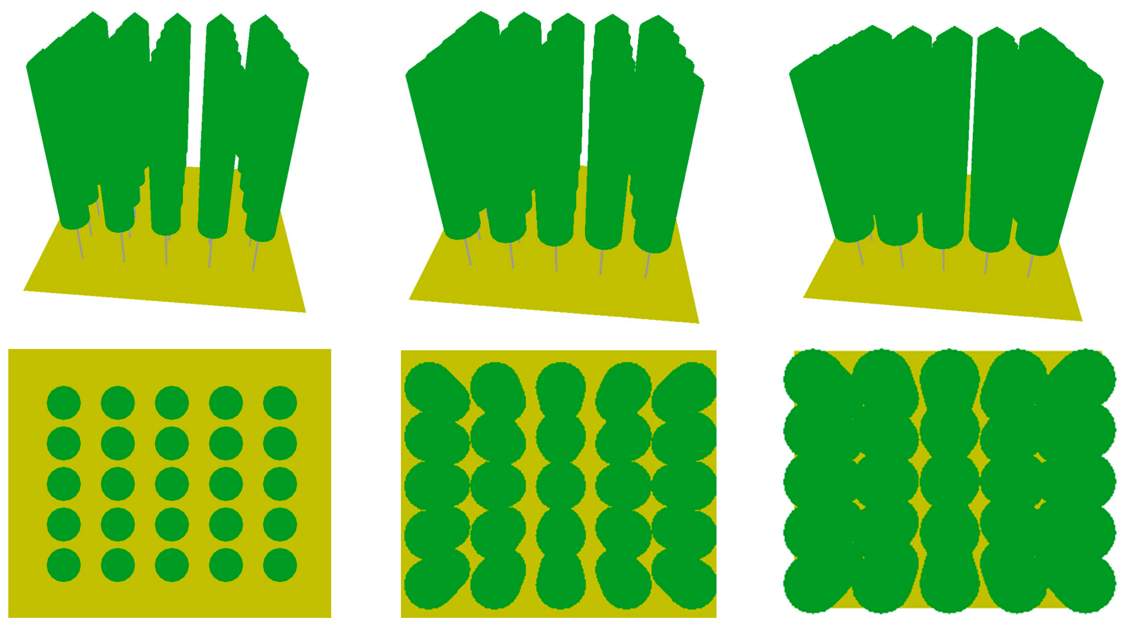
2.1. Three-Dimensional Scene Construction
2.2. SAR and Optical Parameter Settings
2.3. Sensitivity Indicator
3. Results
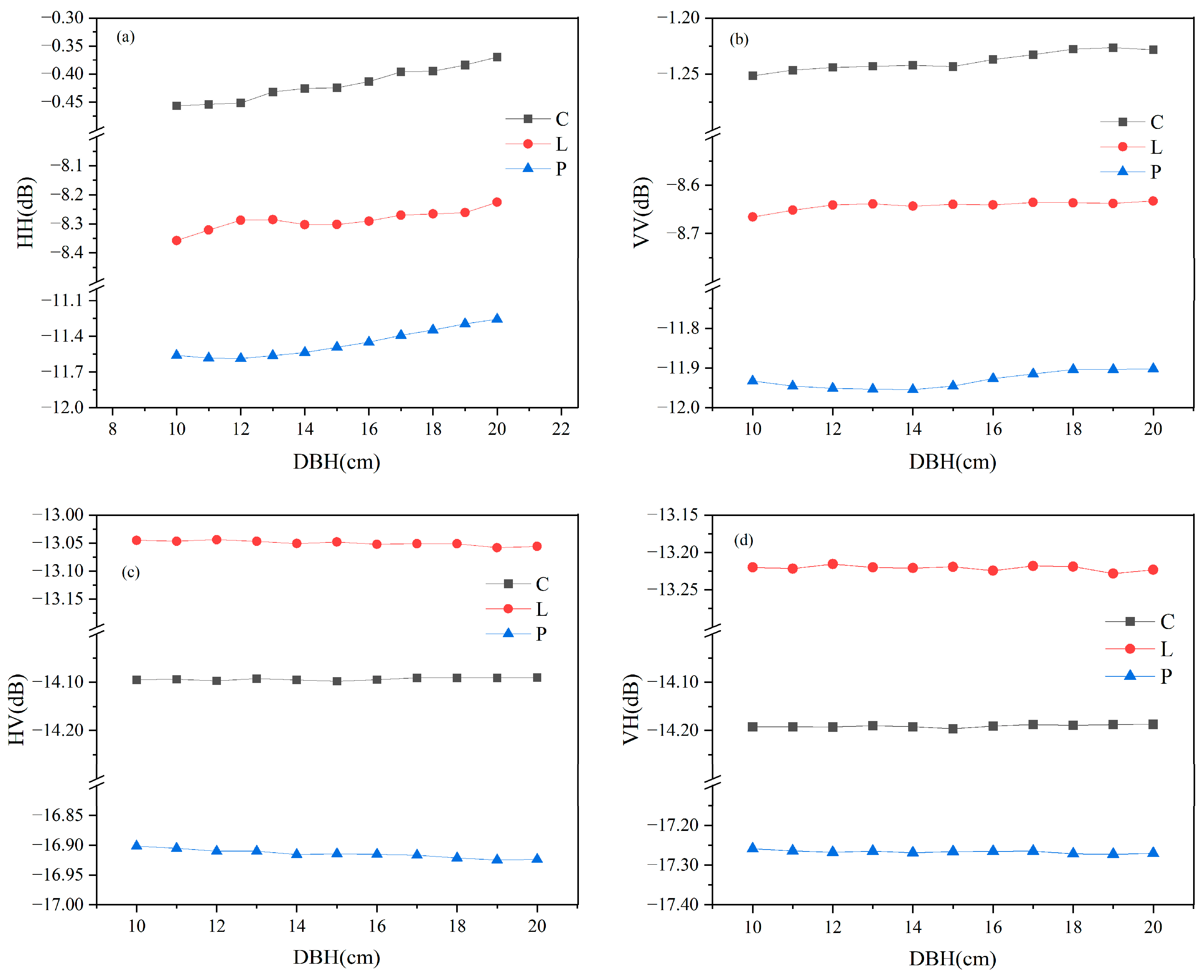
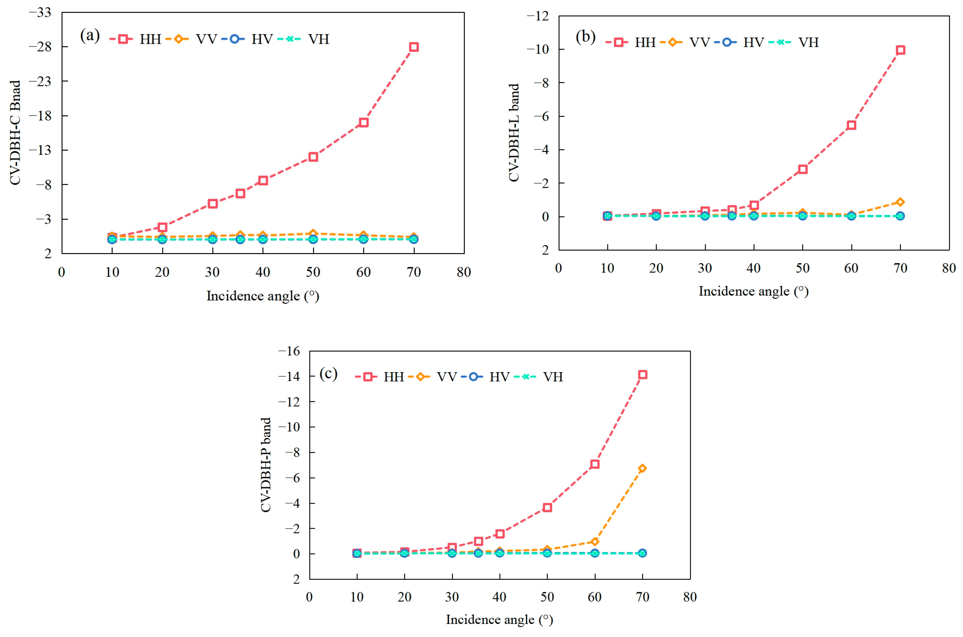
3.1. Diameter at Breast Height
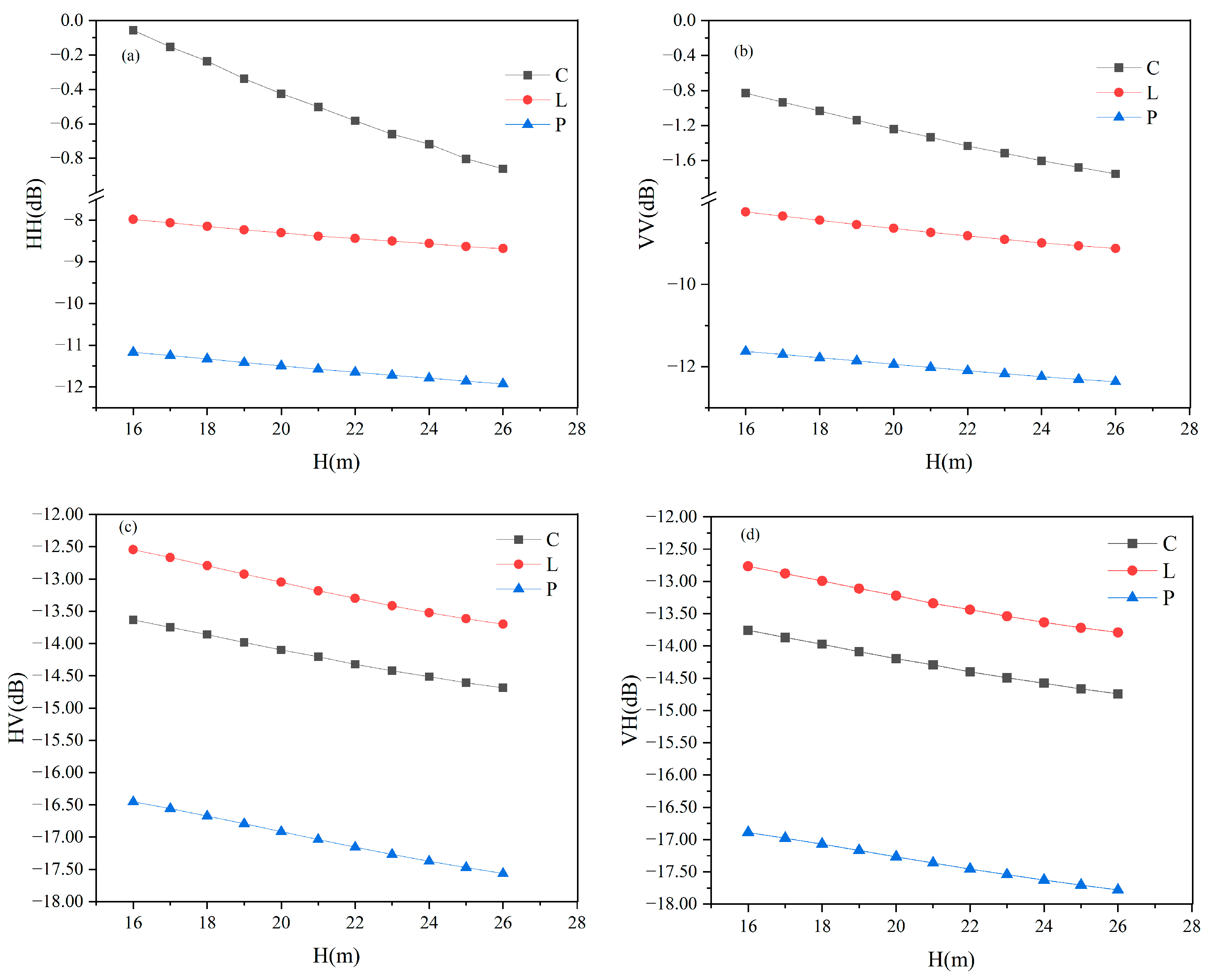
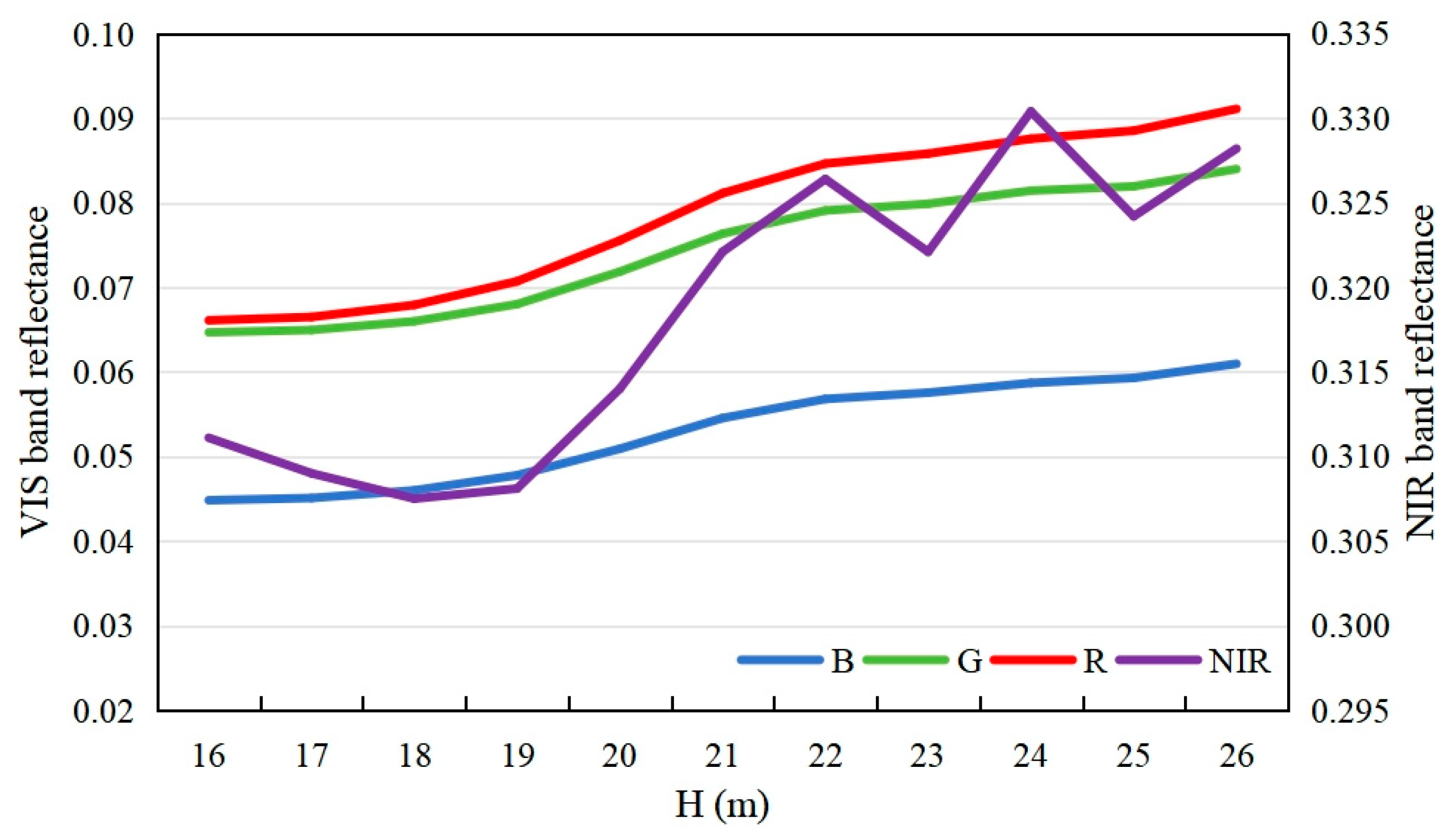
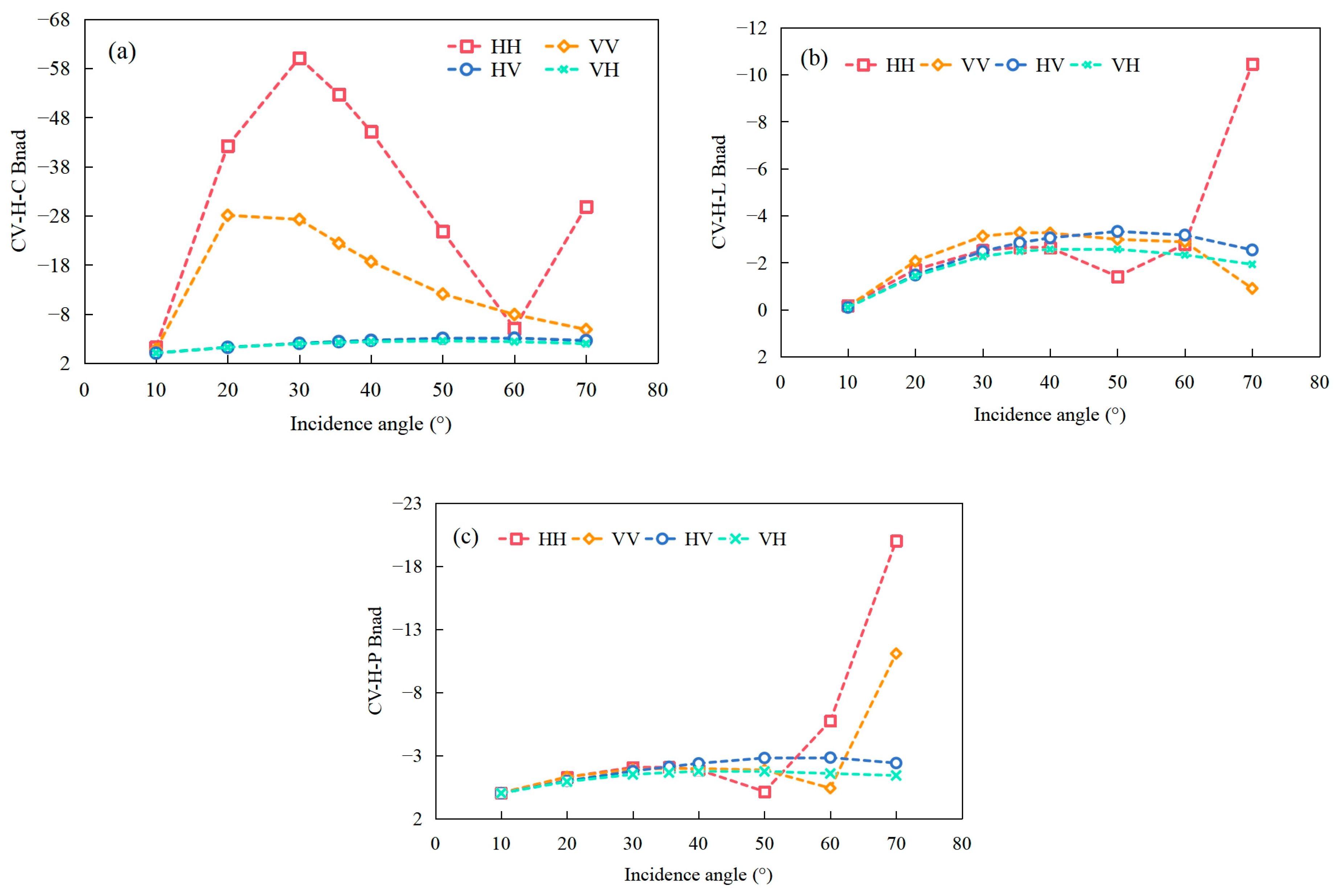
3.2. Height
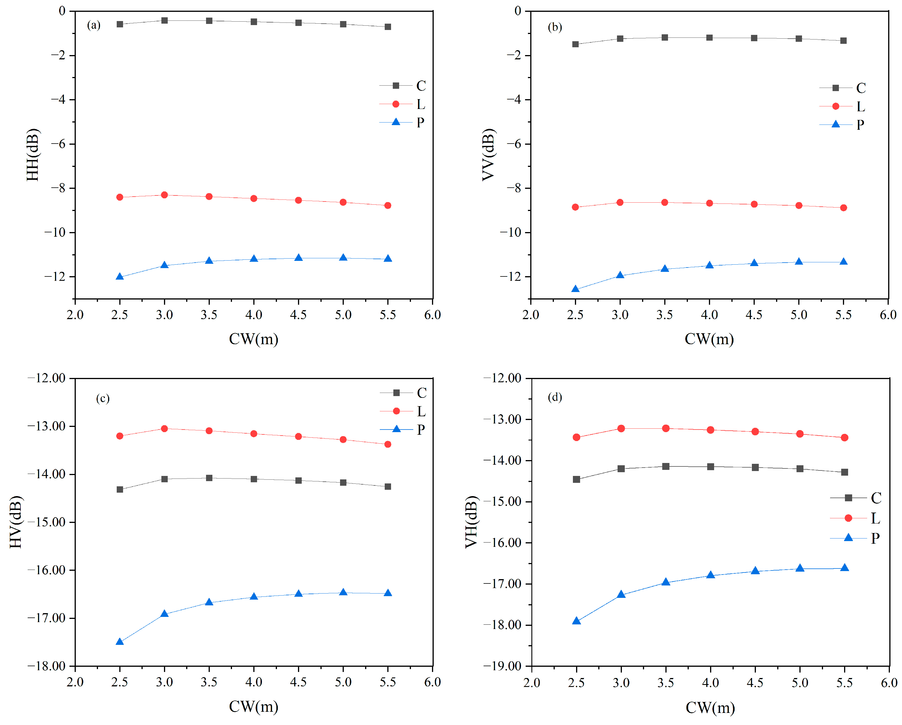
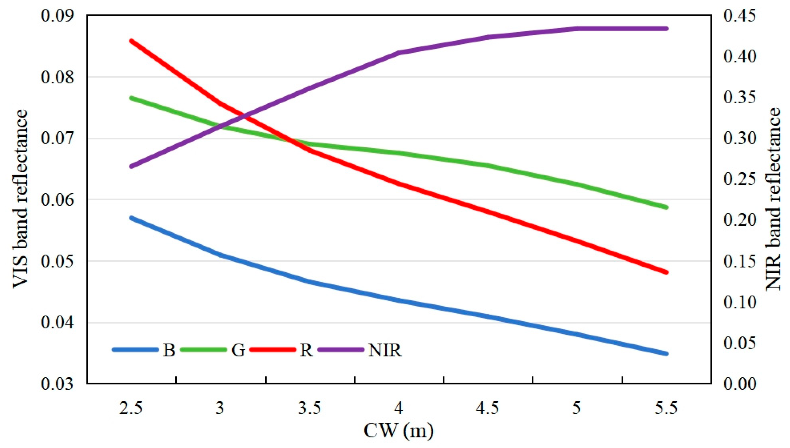
3.3. Crown Width
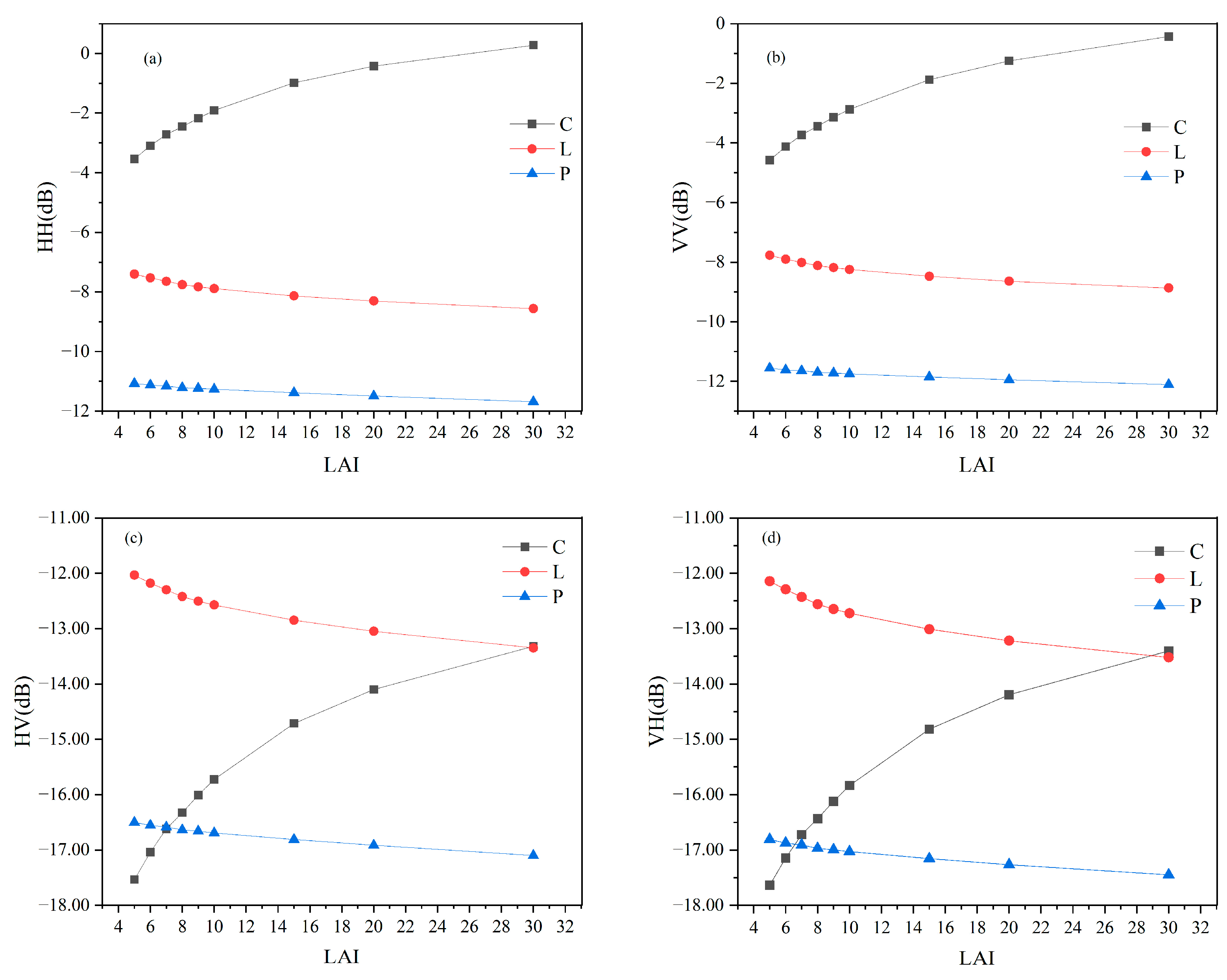
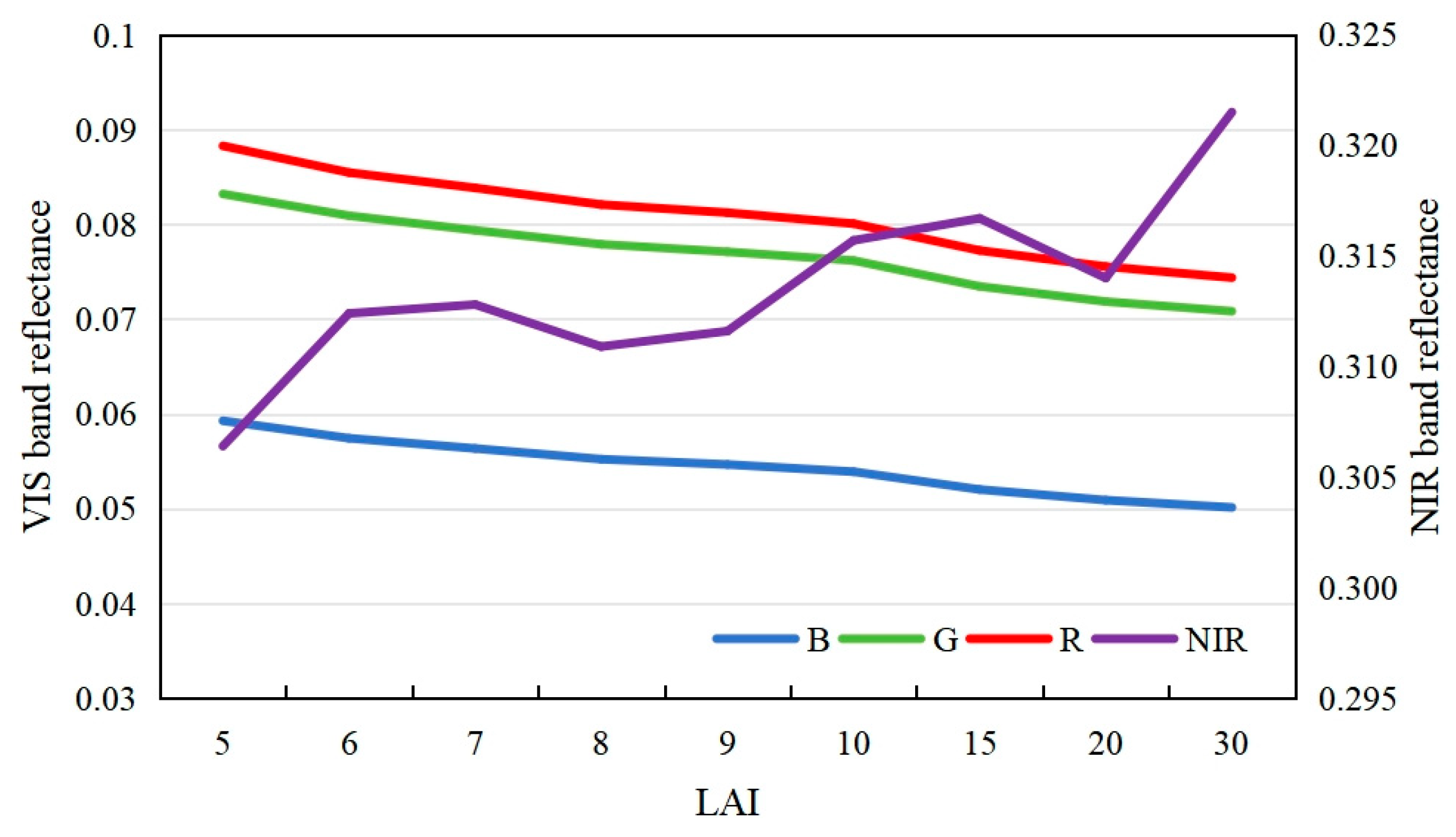
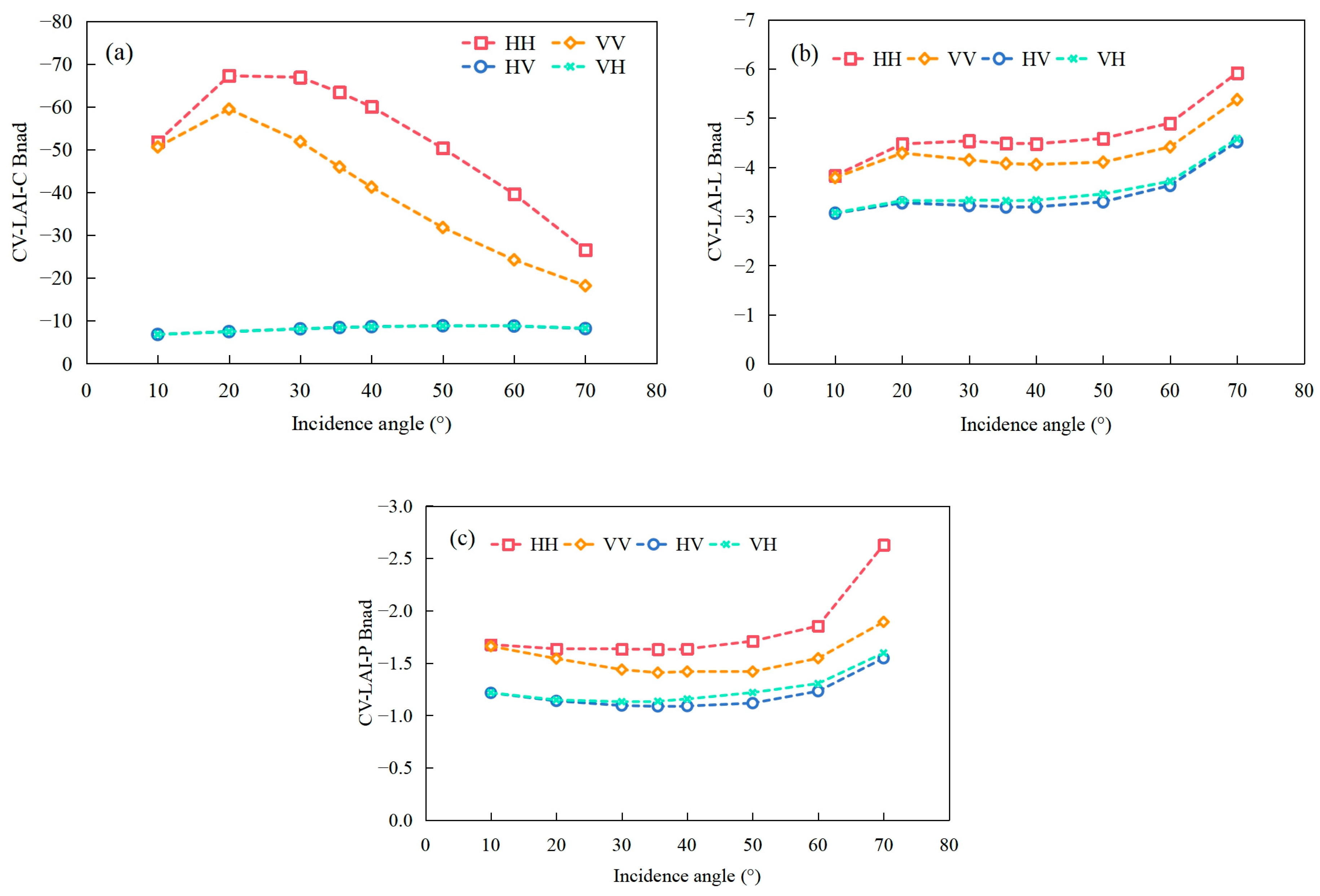
3.4. LAI
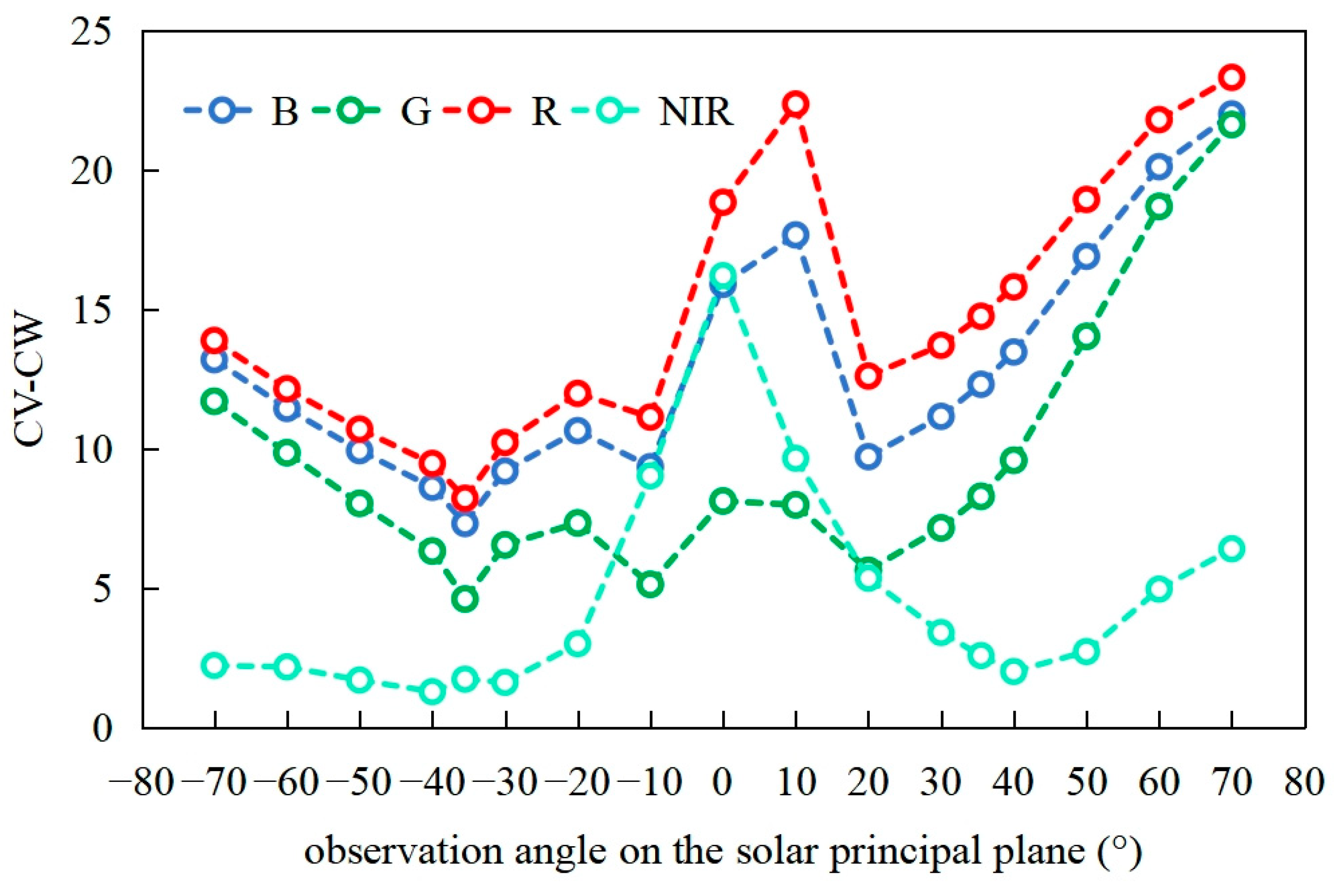
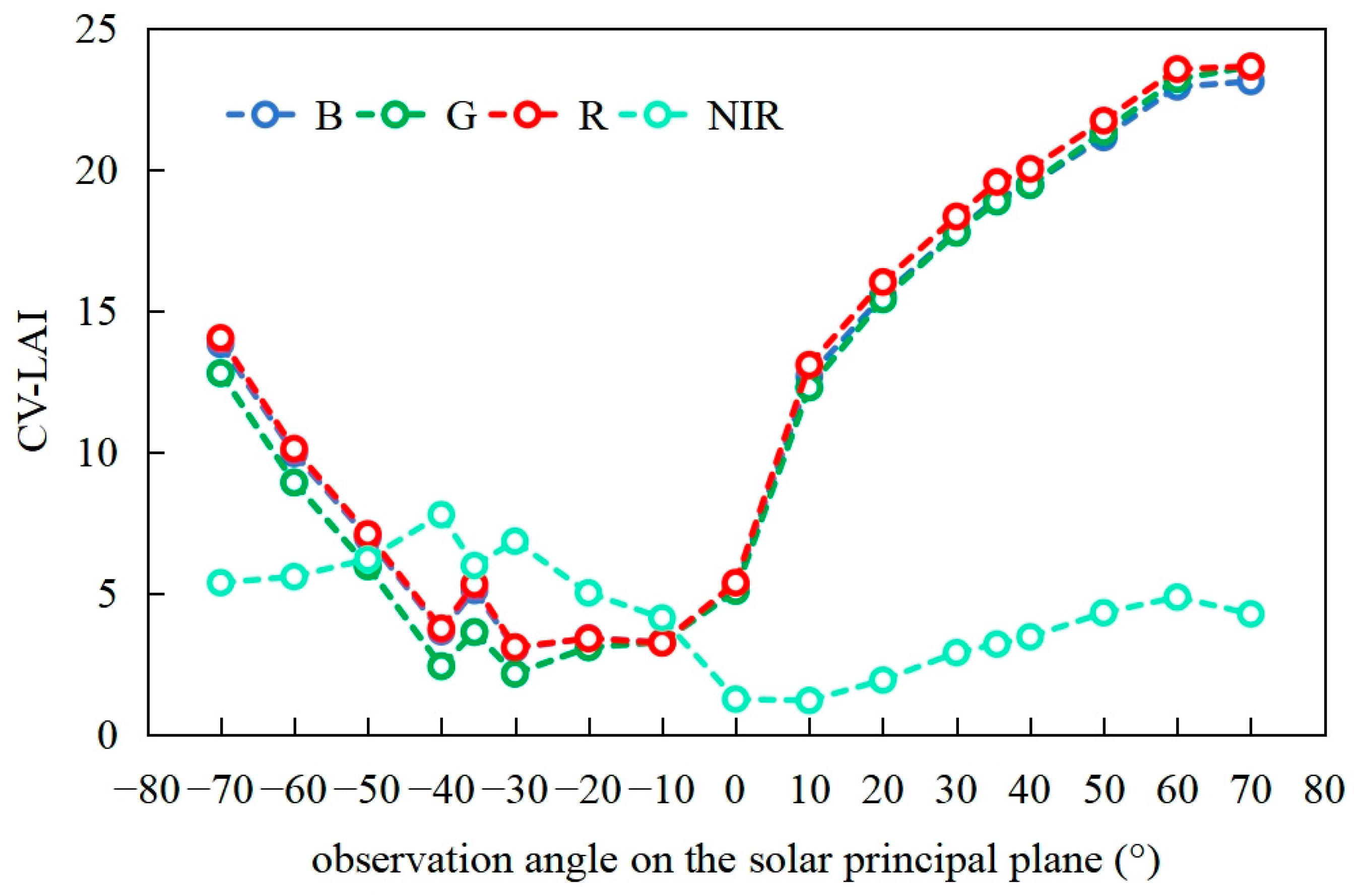
3.5. Sensitivity at Different Angles
4. Discussion
4.1. Sensitivity of SAR Band and Polarization
4.2. Influence of Optical Band Selection
4.3. Effect of SAR Incidence Angle
4.4. Impact of Optical Observation Angle
4.5. Advantages and Challenges
5. Conclusions
Author Contributions
Funding
Data Availability Statement
Acknowledgments
Conflicts of Interest
References
- Shang, R.; Chen, J.M.; Xu, M.; Lin, X.; Li, P.; Yu, G.; He, N.; Xu, L.; Gong, P.; Liu, L.; et al. China’s current forest age structure will lead to weakened carbon sinks in the near future. Innovation 2023, 4, 100515. [Google Scholar] [CrossRef] [PubMed]
- Chen, C.; Park, T.; Wang, X.; Piao, S.; Xu, B.; Chaturvedi, R.K.; Fuchs, R.; Brovkin, V.; Ciais, P.; Fensholt, R. China and India lead in greening of the world through land-use management. Nat. Sustain. 2019, 2, 122–129. [Google Scholar] [CrossRef] [PubMed]
- Wang, Q.; Putri, N.A.; Gan, Y.; Song, G. Combining both spectral and textural indices for alleviating saturation problem in forest LAI estimation using Sentinel-2 data. Geocarto Int. 2022, 37, 10511–10531. [Google Scholar] [CrossRef]
- Huang, Z.; Lv, X.; Li, X.; Chai, H. Maximum a Posteriori Inversion for Forest Height Estimation Using Spaceborne Polarimetric SAR Interferometry. IEEE Trans. Geosci. Remote Sens. 2023, 61, 1–14. [Google Scholar] [CrossRef]
- Tamiminia, H.; Salehi, B.; Mahdianpari, M.; Goulden, T. State-wide forest canopy height and aboveground biomass map for New York with 10 m resolution, integrating GEDI, Sentinel-1, and Sentinel-2 data. Ecol. Inform. 2024, 79, 102404. [Google Scholar] [CrossRef]
- Nguyen, L.V.; Tateishi, R.; Nguyen, H.T.; Sharma, R.C.; Le, S.M. Estimation of Tropical Forest Structural Characteristics Using ALOS-2 SAR Data. Adv. Remote Sens. 2016, 5, 131–144. [Google Scholar] [CrossRef]
- Ji, Y.; Huang, J.; Ju, Y.; Guo, S.; Yue, C. Forest structure dependency analysis of L-band SAR backscatter. PeerJ 2020, 8, e10055. [Google Scholar] [CrossRef]
- Kovacs, J.M.; Jiao, X.; Flores-de-Santiago, F.; Zhang, C.; Flores-Verdugo, F. Assessing relationships between Radarsat-2 C-band and structural parameters of a degraded mangrove forest. Int. J. Remote Sens. 2013, 34, 7002–7019. [Google Scholar] [CrossRef]
- Pereira, L.O.; Furtado, L.F.A.; Novo, E.M.L.M.; Sant Anna, S.J.S.; Liesenberg, V.; Silva, T.S.F. Multifrequency and Full-Polarimetric SAR Assessment for Estimating Above Ground Biomass and Leaf Area Index in the Amazon Várzea Wetlands. Remote Sens. 2018, 10, 1355. [Google Scholar] [CrossRef]
- Schlund, M.; Davidson, M. Aboveground Forest Biomass Estimation Combining L- and P-Band SAR Acquisitions. Remote Sens. 2018, 10, 1151. [Google Scholar] [CrossRef]
- Hu, Y.; Xu, X.; Wu, F.; Sun, Z.; Xia, H.; Meng, Q.; Huang, W.; Zhou, H.; Gao, J.; Li, W.; et al. Estimating Forest Stock Volume in Hunan Province, China, by Integrating In Situ Plot Data, Sentinel-2 Images, and Linear and Machine Learning Regression Models. Remote Sens. 2020, 12, 186. [Google Scholar] [CrossRef]
- Long, J.; Lin, H.; Wang, G.; Sun, H.; Yan, E. Mapping Growing Stem Volume of Chinese Fir Plantation Using a Saturation-based Multivariate Method and Quad-polarimetric SAR Images. Remote Sens. 2019, 11, 1872. [Google Scholar] [CrossRef]
- Timothy, D.; Mutanga, O.; Abdel-Rahman, E.M.; Ismail, R.; Slotow, R. Predicting Eucalyptus spp. stand volume in Zululand, South Africa: An analysis using a stochastic gradient boosting regression ensemble with multi-source data sets. Int. J. Remote Sens. 2015, 36, 3751–3772. [Google Scholar] [CrossRef]
- Dube, T.; Mutanga, O. Investigating the robustness of the new Landsat-8 Operational Land Imager derived texture metrics in estimating plantation forest aboveground biomass in resource constrained areas. ISPRS J. Photogramm. Remote Sens. 2015, 108, 12–32. [Google Scholar] [CrossRef]
- Reuveni, Y.; Dahan, E.; Anker, Y.; Sprintsin, M. Estimating forest parameters using Landsat ETM+ spectral responses and monocultured plantation fieldwork measurements data. Int. J. Remote Sens. 2018, 39, 2620–2636. [Google Scholar] [CrossRef]
- Middinti, S.; Thumaty, K.C.; Gopalakrishnan, R.; Jha, C.S.; Thatiparthi, B.R. Estimating the leaf area index in Indian tropical forests using Landsat-8 OLI data. Int. J. Remote Sens. 2017, 38, 6769–6789. [Google Scholar] [CrossRef]
- Aubry-Kientz, M.; Laybros, A.; Weinstein, B.; Ball, J.; Jackson, T.; Coomes, D.; Vincent, G. Multisensor Data Fusion for Improved Segmentation of Individual Tree Crowns in Dense Tropical Forests. IEEE J. Sel. Top. Appl. Earth Obs. Remote Sens. 2021, 14, 3927–3936. [Google Scholar] [CrossRef]
- Fang, G.; Xu, H.; Yang, S.; Lou, X.; Fang, L. Synergistic use of Sentinel-1, Sentinel-2, and Landsat 8 in predicting forest variables. Ecol. Indic. 2023, 151, 110296. [Google Scholar] [CrossRef]
- Gao, S.; Niu, Z.; Huang, N.; Hou, X. Estimating the Leaf Area Index, height and biomass of maize using HJ-1 and RADARSAT-2. Int. J. Appl. Earth Obs. 2013, 24, 1–8. [Google Scholar] [CrossRef]
- Valero, S.; Arnaud, L.; Planells, M.; Ceschia, E. Synergy of Sentinel-1 and Sentinel-2 Imagery for Early Seasonal Agricultural Crop Mapping. Remote Sens. 2021, 13, 4891. [Google Scholar] [CrossRef]
- Spracklen, B.; Spracklen, D.V. Synergistic Use of Sentinel-1 and Sentinel-2 to Map Natural Forest and Acacia Plantation and Stand Ages in North-Central Vietnam. Remote Sens. 2021, 13, 185. [Google Scholar] [CrossRef]
- Huaguo, H. Principles and Applications of the Three-dimensional Remote Sensing Mechanism Model RAPID. Remote Sens. Technol. Appl. 2019, 34, 901–913. [Google Scholar] [CrossRef]
- Huang, H.; Zhang, Z.; Ni, W.; Chai, L.; Qin, W.; Liu, G.; Xie, D.; Jiang, L.; Liu, Q. Extending RAPID model to simulate forest microwave backscattering. Remote Sens. Environ. 2018, 217, 272–291. [Google Scholar] [CrossRef]
- Gastellu-Etchegorry, J.P.; Lauret, N.; Yin, T.; Landier, L.; Kallel, A.; Malenovsky, Z.; Bitar, A.A.; Aval, J.; Benhmida, S.; Qi, J. DART: Recent Advances in Remote Sensing Data Modeling With Atmosphere, Polarization, and Chlorophyll Fluorescence. IEEE J. Sel. Top. Appl. Earth Obs. Remote Sens. 2017, 10, 2640–2649. [Google Scholar] [CrossRef]
- Huang, H.; Qin, W.; Liu, Q. RAPID: A Radiosity Applicable to Porous IndiviDual Objects for directional reflectance over complex vegetated scenes. Remote Sens. Environ. 2013, 132, 221–237. [Google Scholar] [CrossRef]
- Ferreira, M.P.; Féret, J.; Grau, E.; Gastellu-Etchegorry, J.; Do Amaral, C.H.; Shimabukuro, Y.E.; de Souza Filho, C.R. Retrieving structural and chemical properties of individual tree crowns in a highly diverse tropical forest with 3D radiative transfer modeling and imaging spectroscopy. Remote Sens. Environ. 2018, 211, 276–291. [Google Scholar] [CrossRef]
- Wang, C.; Qi, J. Biophysical estimation in tropical forests using JERS-1 SAR and VNIR imagery. II. Aboveground woody biomass. Int. J. Remote Sens. 2008, 29, 6827–6849. [Google Scholar] [CrossRef]
- Tebaldini, S.; Rocca, F. Multibaseline Polarimetric SAR Tomography of a Boreal Forest at P- and L-Bands. IEEE Trans. Geosci. Remote Sens. 2012, 50, 232–246. [Google Scholar] [CrossRef]
- Ji, Y.; Zhang, F.; Zhang, W.; Zhao, L.; Xu, K.; Shi, J.; Huang, G.; Jing, Q.; Wang, L.; Yang, F. Exploring optimal combinations of multi-frequency polarimetric SAR observations to estimate forest above-ground biomass. Geo-Spat. Inf. Sci. 2024, 28, 629–647. [Google Scholar] [CrossRef]
- Le Toan, T.; Beaudoin, A.; Riom, J.; Guyon, D. Relating forest biomass to SAR data. IEEE Trans. Geosci. Remote Sens. 1992, 30, 403–411. [Google Scholar] [CrossRef]
- Mermoz, S.; Réjou-Méchain, M.; Villard, L.; Le Toan, T.; Rossi, V.; Gourlet-Fleury, S. Decrease of L-band SAR backscatter with biomass of dense forests. Remote Sens. Environ. 2015, 159, 307–317. [Google Scholar] [CrossRef]
- Lal, P.; Kumar, A.; Saikia, P.; Das, A.; Patnaik, C.; Kumar, G.; Pandey, A.C.; Srivastava, P.; Dwivedi, C.S.; Khan, M.L. Effect of vegetation structure on above ground biomass in tropical deciduous forests of Central India. Geocarto Int. 2022, 37, 6294–6310. [Google Scholar] [CrossRef]
- Bousbih, S.; Zribi, M.; Lili-Chabaane, Z.; Baghdadi, N.; El, H.M.; Gao, Q.; Mougenot, B. Potential of Sentinel-1 Radar Data for the Assessment of Soil and Cereal Cover Parameters. Sensors 2017, 17, 2617. [Google Scholar] [CrossRef]
- Huang, W.; Sun, G.; Ni, W.; Zhang, Z.; Dubayah, R. Sensitivity of Multi-Source SAR Backscatter to Changes in Forest Aboveground Biomass. Remote Sens. 2015, 7, 9587–9609. [Google Scholar] [CrossRef]
- Zhang, T.; Lin, H.; Long, J.; Zheng, H.; Ye, Z.; Liu, Z. Evaluating the Sensitivity of Polarimetric Features Related to Rotation Domain and Mapping Chinese Fir AGB Using Quad-Polarimetric SAR Images. Remote Sens. 2023, 15, 1519. [Google Scholar] [CrossRef]
- Rahimizadeh, N.; Sahebi, M.R.; Babaie Kafaky, S.; Mataji, A. Estimation of trees height and vertical structure using SAR interferometry in uneven-aged and mixed forests. Environ. Monit. Assess. 2021, 193, 298. [Google Scholar] [CrossRef]
- He, C.; Tian, X.; Wang, H. Integrating species functional and architectural traits for improving crown width prediction in subtropical multispecies forests using nonlinear hierarchical models. Ecol. Inform. 2025, 90, 103215. [Google Scholar] [CrossRef]
- Bohlin, J.; Wallerman, J.; Fransson, J.E.S.; Sveriges, L. Forest variable estimation using photogrammetric matching of digital aerial images in combination with a high-resolution DEM. Scand. J. For. Res. 2012, 27, 692–699. [Google Scholar] [CrossRef]
- Tompalski, P.; White, J.C.; Coops, N.C.; Wulder, M.A. Quantifying the contribution of spectral metrics derived from digital aerial photogrammetry to area-based models of forest inventory attributes. Remote Sens. Environ. 2019, 234, 111434. [Google Scholar] [CrossRef]
- Mao, Z.; Lu, Z.; Wu, Y.; Deng, L. DBH Estimation for Individual Tree: Two-Dimensional Images or Three-Dimensional Point Clouds? Remote Sens. 2023, 15, 4116. [Google Scholar] [CrossRef]
- Shamsoddini, A.; Trinder, J.C.; Turner, R. Pine plantation structure mapping using WorldView-2 multispectral image. Int. J. Remote Sens. 2013, 34, 3986–4007. [Google Scholar] [CrossRef]
- Heiskanen, J. Tree cover and height estimation in the Fennoscandian tundra–taiga transition zone using multiangular MISR data. Remote Sens. Environ. 2006, 103, 97–114. [Google Scholar] [CrossRef]
- Pu, R.; Landry, S. Evaluating seasonal effect on forest leaf area index mapping using multi-seasonal high resolution satellite pleiades imagery. Int. J. Appl. Earth Obs. 2019, 80, 268–279. [Google Scholar] [CrossRef]
- Salazar-Neira, J.C.; Mialon, A.; Richaume, P.; Mermoz, S.; Kerr, Y.H.; Bouvet, A.; Le Toan, T.; Boitard, S.; Rodríguez-Fernández, N.J. Above-Ground Biomass Estimation Based on Multi-Angular L-Band Measurements of Brightness Temperatures. IEEE J. Sel. Top. Appl. Earth Obs. Remote Sens. 2023, 16, 5813–5827. [Google Scholar] [CrossRef]
- Lu, D.; Chen, Q.; Wang, G.; Liu, L.; Li, G.; Moran, E. A survey of remote sensing-based aboveground biomass estimation methods in forest ecosystems. Int. J. Digit. Earth 2014, 9, 63–105. [Google Scholar] [CrossRef]
- Yongjie, J.; Congrui, Y.; Wangfei, Z.; Peng, Z.; Fuxiang, Z.; Ya’Ni, Q. Forest above ground biomass estimation using airborne P band polarimetric SAR data. J. Zhejiang A F Univ. 2022, 39, 971–980. [Google Scholar] [CrossRef]
- Cartus, O.; Santoro, M.; Wegmueller; Rommen, B. Benchmarking the Retrieval of Biomass in Boreal Forests Using P-Band SAR Backscatter with Multi-Temporal C- and L-Band Observations. Remote Sens. 2019, 11, 1695. [Google Scholar] [CrossRef]
- Qi, F.; Erxue, C.; Zengyuan, L.; Lan, L.; Lei, Z. Forest Above-Ground Biomass Estimation Method for Rugged Terrain Based on Airborne P-Band PolSAR Data. Sci. Silvae Sin. 2016, 52, 13. [Google Scholar] [CrossRef]
- Bartalev, S.A.; Belward, A.S.; Isaev, D.V.E.A. A new SPOT4-VEGETATION derived land cover map of Northern Eurasia. Int. J. Remote Sens. 2003, 24, 1977–1982. [Google Scholar] [CrossRef]
- Deering, S.S.W. Structure Analysis and Classification of Boreal Forests Using Airborne Hyperspectral BRDF Data from ASAS. Remote Sens. Environ. 1999, 69, 281–295. [Google Scholar] [CrossRef]
- Abuelgasim, A.A.; Gopal, S.; Irons, J.R.; Strahler, A.H. Classification of ASAS multiangle and multispectral measurements using artificial neural networks. Remote Sens. Environ. 1996, 57, 79–87. [Google Scholar] [CrossRef]
- Gemmell, F. Testing the utility of multi-angle spectral data for reducing the effects of background spectral variations in forest reflectance model inversion. Remote Sens. Environ. 2000, 72, 46–63. [Google Scholar] [CrossRef]
- Disney, M.; Lewis, P.; Saich, P. 3D modelling of forest canopy structure for remote sensing simulations in the optical and microwave domains. Remote Sens. Environ. 2006, 100, 114–132. [Google Scholar] [CrossRef]
- Sexton, J.O.; Song, X.; Feng, M.; Noojipady, P.; Anand, A.; Huang, C.; Kim, D.; Collins, K.M.; Channan, S.; DiMiceli, C.; et al. Global, 30-m resolution continuous fields of tree cover: Landsat-based rescaling of MODIS vegetation continuous fields with lidar-based estimates of error. Int. J. Digit. Earth 2013, 6, 427–448. [Google Scholar] [CrossRef]
- Leng, Y.; Li, W.; Ciais, P.; Sun, M.; Zhu, L.; Yue, C.; Chang, J.; Yao, Y.; Zhang, Y.; Zhou, J.; et al. Forest aging limits future carbon sink in China. One Earth 2024, 7, 822–834. [Google Scholar] [CrossRef]
- Mermoz, S.; Le Toan, T.; Villard, L.; Réjou-Méchain, M.; Seifert-Granzin, J. Biomass assessment in the Cameroon savanna using ALOS PALSAR data. Remote Sens. Environ. 2014, 155, 109–119. [Google Scholar] [CrossRef]


| Model Input | Range | Default Value |
|---|---|---|
| DBH | 10–20 cm, step size 1 cm | 15 |
| H | 16–26 m, step size 1 m | 20 |
| CW | 2.5–5.5 m, step size 0.5 m | 3 |
| LAI | 5–10 (step size 1), 15, 20, 30 | 20 |
| DBH | C | L | P | |
|---|---|---|---|---|
| HH | min | −0.457 | −8.358 | −11.587 |
| max | −0.370 | −8.225 | −11.258 | |
| range | 0.087 | 0.132 | 0.329 | |
| CV(%) | −6.73 | −0.40 | −1.00 | |
| VV | min | −1.252 | −8.666 | −11.954 |
| max | −1.226 | −8.633 | −11.902 | |
| range | 0.025 | 0.033 | 0.052 | |
| CV(%) | −0.66 | −0.10 | −0.17 | |
| HV | min | −14.098 | −13.058 | −16.925 |
| max | −14.090 | −13.044 | −16.901 | |
| range | 0.008 | 0.014 | 0.024 | |
| CV(%) | −0.02 | −0.03 | −0.04 | |
| VH | min | −14.196 | −13.228 | −17.273 |
| max | −14.187 | −13.216 | −17.259 | |
| range | 0.009 | 0.013 | 0.014 | |
| CV(%) | −0.02 | −0.02 | −0.02 |
| H | C | L | P | |
|---|---|---|---|---|
| HH | min | −0.861 | −8.680 | −11.928 |
| max | −0.056 | −7.982 | −11.170 | |
| range | 0.805 | 0.697 | 0.758 | |
| CV(%) | −52.68 | −2.65 | −2.09 | |
| VV | min | −1.754 | −9.128 | −12.367 |
| max | −0.830 | −8.239 | −11.631 | |
| range | 0.924 | 0.889 | 0.736 | |
| CV(%) | −22.38 | −3.27 | −1.98 | |
| HV | min | −14.688 | −13.698 | −17.564 |
| max | −13.633 | −12.545 | −16.451 | |
| range | 1.054 | 1.153 | 1.113 | |
| CV(%) | −2.39 | −2.84 | −2.11 | |
| VH | min | −14.741 | −13.791 | −17.780 |
| max | −13.757 | −12.765 | −16.890 | |
| range | 0.985 | 1.026 | 0.890 | |
| CV(%) | −2.21 | −2.49 | −1.65 |
| CW | C | L | P | |
|---|---|---|---|---|
| HH | min | −0.706 | −8.777 | −12.011 |
| max | −0.425 | −8.302 | −11.154 | |
| range | 0.281 | 0.475 | 0.857 | |
| CV(%) | −17.26 | −1.79 | −2.54 | |
| VV | min | −1.495 | −8.879 | −12.571 |
| max | −1.198 | −8.639 | −11.336 | |
| range | 0.298 | 0.240 | 1.235 | |
| CV(%) | −7.74 | −1.05 | −3.57 | |
| HV | min | −14.316 | −13.374 | −17.499 |
| max | −14.076 | −13.048 | −16.468 | |
| range | 0.241 | 0.326 | 1.031 | |
| CV(%) | −0.60 | −0.77 | −2.07 | |
| VH | min | −14.457 | −13.440 | −17.913 |
| max | −14.141 | −13.216 | −16.620 | |
| range | 0.316 | 0.224 | 1.292 | |
| CV(%) | −0.73 | −0.66 | −2.56 |
| LAI | C | L | P | |
|---|---|---|---|---|
| HH | min | −3.539 | −8.559 | −11.680 |
| max | 0.279 | −7.406 | −11.072 | |
| range | 3.818 | 1.153 | 0.608 | |
| CV(%) | −63.39 | −4.48 | −1.63 | |
| VV | min | −4.577 | −8.868 | −12.107 |
| max | −0.432 | −7.771 | −11.559 | |
| range | 4.144 | 1.097 | 0.548 | |
| CV(%) | −45.95 | −4.07 | −1.41 | |
| HV | min | −17.535 | −13.347 | −17.101 |
| max | −13.321 | −12.034 | −16.502 | |
| range | 4.214 | 1.313 | 0.599 | |
| CV(%) | −8.41 | −3.19 | −1.09 | |
| VH | min | −17.640 | −13.520 | −17.449 |
| max | −13.402 | −12.145 | −16.809 | |
| range | 4.239 | 1.375 | 0.640 | |
| CV(%) | −8.39 | −3.31 | −1.13 |
Disclaimer/Publisher’s Note: The statements, opinions and data contained in all publications are solely those of the individual author(s) and contributor(s) and not of MDPI and/or the editor(s). MDPI and/or the editor(s) disclaim responsibility for any injury to people or property resulting from any ideas, methods, instructions or products referred to in the content. |
© 2025 by the authors. Licensee MDPI, Basel, Switzerland. This article is an open access article distributed under the terms and conditions of the Creative Commons Attribution (CC BY) license (https://creativecommons.org/licenses/by/4.0/).
Share and Cite
Mao, Z.; Deng, L.; Liu, X.; Wang, Y. A Comparative Analysis of SAR and Optical Remote Sensing for Sparse Forest Structure Parameters: A Simulation Study. Forests 2025, 16, 1244. https://doi.org/10.3390/f16081244
Mao Z, Deng L, Liu X, Wang Y. A Comparative Analysis of SAR and Optical Remote Sensing for Sparse Forest Structure Parameters: A Simulation Study. Forests. 2025; 16(8):1244. https://doi.org/10.3390/f16081244
Chicago/Turabian StyleMao, Zhihui, Lei Deng, Xinyi Liu, and Yueyang Wang. 2025. "A Comparative Analysis of SAR and Optical Remote Sensing for Sparse Forest Structure Parameters: A Simulation Study" Forests 16, no. 8: 1244. https://doi.org/10.3390/f16081244
APA StyleMao, Z., Deng, L., Liu, X., & Wang, Y. (2025). A Comparative Analysis of SAR and Optical Remote Sensing for Sparse Forest Structure Parameters: A Simulation Study. Forests, 16(8), 1244. https://doi.org/10.3390/f16081244