Article

Treeline Species Distribution Under Climate Change: Modelling the Current and Future Range of Nothofagus pumilio in the Southern Andes

1
Institute of Geography, Center for Earth System Research and Sustainability (CEN), University of Hamburg, Bundesstraße 55, 20146 Hamburg, Germany
2
Institute of Geography, Cluster of Excellence “Climate, Climatic Change, and Society” (CLICCS), Center for Earth System Research and Sustainability (CEN), University of Hamburg, Bundesstraße 55, 20146 Hamburg, Germany
3
Institute for Globally Distributed Open Research and Education (IGDORE), Burgunderweg 9d, 22453 Hamburg, Germany
*
Author to whom correspondence should be addressed.
Forests 2025, 16(8), 1211; https://doi.org/10.3390/f16081211
Submission received: 23 May 2025 / Revised: 18 July 2025 / Accepted: 21 July 2025 / Published: 23 July 2025
(This article belongs to the Section Forest Ecology and Management)

Abstract

Although treeline ecotones are significant components of vulnerable mountain ecosystems and key indicators of climate change, treelines of the Southern Hemisphere remain largely outside of research focus. In this study, we investigate, for the first time, the current and future distribution of the treeline species Nothofagus pumilio in the Southern Andes using a Species Distribution Modelling approach. The lack of modelling studies in this region can be contributed to missing occurrence data for the species. In a preliminary study, both point and raster data were generated using a novel Instagram ground truthing approach and remote sensing. Here we tested the performance of the two datasets: a typical binary species dataset consisting of occurrence points and pseudo-absence points and a continuous dataset where species occurrence was determined by supervised classification. We used a Random Forest (RF) classification and a RF regression approach. RF is applicable for both datasets, has a very good performance, handles multicollinearity and remains largely interpretable. We used bioclimatic variables from CHELSA as predictors. The two models differ in terms of variable importance and spatial prediction. While a temperature variable is the most important variable in the RF classification, the RF regression model was mainly modelled by precipitation variables. Heat deficiency is the most important limiting factor for tree growth at treelines. It is evident, however, that water availability and drought stress will play an increasingly important role for the future competitiveness of treeline species and their distribution. Modelling with binary presence–absence point data in the RF classification model led to an overprediction of the potential distribution of the species in summit regions and in glacier areas, while the RF regression model, trained with continuous raster data, led to a spatial prediction with small-scale details. The time-consuming and costly acquisition of complex species information should be accepted in order to provide better predictions and insights into the potential current and future distribution of a species.

1. Introduction

The application of modelling approaches, including Species Distribution Modelling (SDM), has recently rapidly increased in order to generate insights into the sensitivity and shifts in treelines in response to climate change [1]. Warming rates in high mountain regions are, on average, greater than the global mean, resulting in ecosystems being particularly stressed by changing climatic conditions [2]. The natural elevational position of the treeline is defined by heat deficiency [3] and, globally, is approximately aligned with the 6.4 °C isotherm [4]. Consequently, treeline shift in response to warming is frequently investigated and widely recognised as a key indicator of climate change [5]. However, observed responses are rather inconsistent, spanning the entire gradient from static treelines with insignificant responses to dynamic treelines with substantial treeline advance [6,7,8]. Globally, the proportion of advancing elevational treelines has been increasing from 52% [9] to 66% [10,11]. In the Northern Hemisphere, 90% of treelines are reported to be advancing [12], whereas treelines in the Southern Hemisphere are responding weakly to climatic changes [11]. Certain relationships between treeline form, which can vary between gradual and abrupt, and treeline dynamics have been suggested [13]. Factors such as seedling mortality and dieback processes play critical roles in shaping treeline form and influencing possible shifts [14]. While gradual treelines are more likely to advance to higher elevations, abrupt treelines, as formed by Nothofagus in the Southern Hemisphere, are more stable due to increased seedling mortality above closed forest stands or due to anthropogenic disturbances [14].
Treelines and the shift in treelines have extensively been studied in recent decades [1,15]; however, comparatively few studies focused on treelines of the Southern Hemisphere [10,11]. A recent review study examining the impact of climate change on Andean biomes found that those in the southern Andes remain the least studied [16]. For example, to our knowledge, there is no SDM study investigating the entire current and future distribution of important treeline species in the Southern Andes. Nothofagus pumilio (Poepp et Endl.) Krasser (southern or lenga beech) is forming an abrupt treeline over approximately 2000 km latitudinal extent from 35° S to 56° S in the Southern Andes. The treeline is naturally abrupt due to seedling dieback outside the protecting tree stands [17], and in some cases the treeline is influenced by anthropogenic disturbances like grazing, forestry or fire, resulting in more diffuse treeline ecotones [14]. The uppermost trees are often in a krummholz growth form [18]. The treeline follows a 6.6 °C isotherm [19], while increases from 1.2 to 4.0 °C in mean annual temperatures and decreases of up to 30% in mean annual precipitation are predicted for high-elevation catchments in the southern Andes [20,21]. It is therefore of interest to study the changes in the Southern Andean treeline as a result of global warming.
Recent research has explored changes at the treeline of N. pumilio through small-scale dendrochronological and experimental studies [22,23,24,25,26]. N. pumilio is highly sensitive to variations in temperature and precipitation, which are often associated with phase shifts in Antarctic Decadal Oscillation (AAO) also known as the Southern Annular Mode (SAM), the El Niño Southern Oscillation (ENSO), and Pacific Decadal Oscillation (PDO), as highlighted in recent studies [22,23,24]. Increases in radial growth due to rising temperatures have been observed when precipitation levels are sufficient [22,25,26]. Warm and dry springs lead to an increased tree growth at humid treeline sites but to a decrease in tree growth and an increase in tree mortality due to drought at drier treeline sides. Furthermore, high precipitation in late spring often connected with a prolonged snow cover results in a decrease in tree growth [22]. Accordingly, tree growth is highest at mesic sites, followed by wetter sites, while growth rates at drier sites continue to decline [25]. Suitable climatic conditions, particularly rising mean spring and summer temperatures, also promote the establishment of N. pumilio seedlings above the current treeline, on both humid and dry slopes, thereby facilitating treeline advance [23,24]. Additionally, warmer springs can improve seed quantity and quality [27] which further increases the possibility of seedlings becoming established. However, drought or soils with low water capacity are important controlling factors, causing drought stress for seedlings and adult trees [28] and ultimately preventing a treeline advance.
In this study, we model the potential current and future distribution of N. pumilio based on the species’ suitable bioclimatic conditions, following fundamental concepts of Species Distribution Modelling (SDM). SDM models are typically constructed using binary species occurrence data and environmental variables, often climate data [29]. While global climate datasets, such as the CHELSA bioclimatic variables that we use here [30,31], are readily available, the availability of unbiased species occurrence data is a major challenge for SDM studies. Field studies, which can generate reliable occurrence data, are both time-consuming and costly. Moreover, many study sites, particularly in topographic complex regions like high mountains are inaccessible. When species data are not collected through field studies, they are primarily obtained from open-source databases such as the Global Biodiversity Information Facility (GBIF). Although the quantity [32] and quality [33] of data in databases are increasing, these sources often still contain various forms of bias, as highlighted in recent studies [34,35]. Consequently, using these point occurrences in SDM approaches, without addressing these issues, can lead to inaccurate or misleading model results [36]. A promising approach for the investigation of large study areas, especially in regions with limited accessibility, is the use of remote sensing to survey species occurrences [37,38,39]. Remote sensing data on a species can provide more complex, continuous data and thus further modelling opportunities. However, there is still a need for ground truthing to verify that the species of interest are actually present in the remotely sensed area. In a previous study, we developed an Instagram ground truthing approach, that created less-biased occurrence points, that were subsequently used to validate remote sensing occurrence data of N. pumilio, resulting in two valid occurrence datasets [40].
Here, we present an initial holistic approach to model the potential distribution of N. pumilio based on two input datasets: a binary point dataset and a continuous raster occurrence dataset derived from supervised classification. While we adopted a standard modelling approach, we also test an innovative technique incorporating continuous raster data. We hypothesise that this approach will yield more detailed insights into the species’ potential current and future distribution due to the increased complexity of input data.
To investigate the effect of different species input datasets, our aims are (1) to model the current distribution of N. pumilio under prevailing climate conditions, and (2) assess potential range shifts under climate change conditions, and (3) evaluate model performance and model complexity with regard to ecological site factors.

2. Materials and Methods

2.1. Study Species and Study Area

N. pumilio is the most orophilous and widespread species of the Nothofagus genus on the South American continent, extending from 35° S to the southernmost tip of Tierra del Fuego (see Figure 1). As an indicator of the orotemperate belt, it forms mono-species forests at the treeline [41]. The species is sometimes accompanied by the morphologically and ecologically similar species N. antarctica, with which it can form mixed stands. Hybrids between the two species are also known [42]. The evergreen N. betuloides dominates in the lowlands and especially in the (hyper-) humid west.
The study area is characterised by two extreme gradients. One is the temperature gradient, which results from the elevation of the southern Andean Cordillera (up to 3000 m), and the other is the precipitation gradient, which is considered to be the most extreme precipitation gradient on Earth. While precipitation extremes of up to 10,000 mm/year occur on the windward side, west of the Andes, there is a precipitation decrease to less than 300 mm/year on the leeward side, east of the Andes [43]. Northern Patagonia has been substantially affected by the effects of climate change. Mean annual temperatures have risen by up to 1 °C since 1950. While there are no negative trends in precipitation in most areas, precipitation totals are decreasing by 5% in Northern Patagonia. Climate models predict a decrease in precipitation of up to 30% and an increase in temperature of between 1.5 and 3 °C [21].

2.2. Input Data

2.2.1. Species Data

The two species occurrence datasets used were generated in a previous study using a novel Instagram ground truthing approach (IGTA, [40]) designed to reduce sampling and spatial bias often present in existing databases [34,44]. The IGTA aimed at reducing this bias by using a very public and worldwide used social media platform (https://www.instagram.com/) and by including remote sensing data. The study species and area are particularly well-suited for an Instagram-based analysis, as deciduous N. pumilio forms mono-species forests at the treeline, making it an especially attractive photo motif in autumn and occurs in a highly touristic region, where tourists and hikers frequently take and share photos on social media. We compiled 1238 occurrence points extending from 36.88° S to 55.03° S by searching for suitable posts uploaded between 2017 and 2022 with the species and the photos’ location clearly identifiable, as well as a strict catalogue of criteria. Spatial bias commonly present in datasets derived from citizen science or social media, typically due to sampling near urban centres or in easily accessible areas [45,46], was reduced through the IGTA. This reduction in bias is primarily due to the high number of posts, which included not only intentional but also incidental records of the species. Furthermore, owing to the ecology and phenology of N. pumilio, occurrence points were identifiable not only at the exact location where the photo was taken, but also in the background, where the abrupt treeline and the species’ autumn colouring were visible. Although some spatial bias remains, since posts are still limited to human-accessible areas, analysis using the R package “sampbias” (version 2.0.0) [47] indicates that the bias was effectively reduced in comparison to 558 points (after filtering for missing coordinates and a coordinate uncertainty of 1 km) from often used open-source database Global Biodiversity Information Facility (GBIF). In addition, the manual georeferencing of occurrence points further reduced coordinate uncertainty. To minimise spatial bias, remote sensing data generated using Sentinel-2 level 2A data and supervised classification were created and subsequently validated using the IGTA occurrence points as ground truth. Training areas were defined and trained using all relevant spectral bands (bands 2 to 7, 8a, 11, and 12) at a spatial resolution of 20 m. Only vegetation raster cells were included in the supervised classification, which distinguished between three classes (deciduous vegetation/N. pumilio, evergreen vegetation, and low vegetation/grassland). An altitude correction was applied to ensure that only deciduous vegetation in high elevation was classified as N. pumilio. With this approach, two datasets were created: a point occurrence dataset and a spatial raster dataset of the species N. pumilio (Figure 1).
For the IGTA point dataset, the first step in modelling was to ensure that only one point was set in a raster cell at the target resolution of 30 arc sec, ~1 km (raster cell size of the climate data). After deleting duplicate points, 999 points remained in the model as “presence” data. For “absence” data, 2000 pseudo-absence points (PA) were generated. The number and the location of PA points have great influence on the model output [48]. We initially tested a PA ratio of 1:1 as suggested for RF models in relevant literature [49]. However, using only 1000 PA points across a large study area resulted in substantial overprediction by the RF classification model, a known issue [49]. Consequently, we adopted a ratio of 1:2 (2000 PA points). The process of PA creation involved first constructing an alpha hull around the presence points and applying a 1 km buffer, within which PA points were randomly generated. To prevent the overwriting of occurrence cells during this process, a 5 km buffer was placed around the presence points. For the final modelling dataset, values from the climate dataset were extracted for both presence and absence points. The two datasets were then merged and supplemented with a binary indicator variable specifying whether N. pumilio was present (presence = 1) or absent (absence = 0).
The second dataset was derived from a supervised classification (Kappa values: summer scenes classification 0.89, autumn scenes classification 0.96), in which occurrences of deciduous forest at the treeline were classified to represent the distribution of N. pumilio [40]. Gaps in the dataset resulted from missing Sentinel-2 data or areas affected by shadows and cloud cover. The original dataset has a spatial resolution of 20 m. For modelling purposes, N. pumilio cover values were aggregated to the target resolution (~1 km), resulting in percentage values ranging from close to 0% up to a maximum of 99.96%. The raster data covers a latitudinal range from 33.49° S to 56.27° S.

2.2.2. Bioclimatic Predictors

Global climatological datasets such as CHELSA [30,31] and Worldclim [50,51] are standards for large-scale SDM studies. Due to their free accessibility, the datasets are widely used and cited, allowing for some comparability of modelling studies. Since other studies suggest that the CHELSA dataset performs better in topographically highly complex areas such as high mountains [52,53], we decided to use this dataset. We utilised the 19 Bioclim variables from version 2.1 with a 30 arc sec (~1 km) resolution [30,31]. The dataset includes temperature and precipitation variables calculated on a daily, monthly, or annual basis, averaged from climate records for the period 1981 to 2010. The “ClimDatDownloadR” R package was used to download and pre-process the data (version 0.1.7.6) [54,55]. As the Bioclim variables were highly multicollinear, we decided to use a subset of the data. To enhance ecological interpretability, we included only variables derived for quarters. This allows for a better ecological understanding of the bioclimatic conditions at the treeline than variables for individual months or annual averages, as conclusions can be drawn about seasonality [56]. At high elevations, the growth and survival of treeline species are primarily determined by conditions during the short growing season [1]. Quarterly variables can isolate this critical period, whereas annual means combine summer and winter extremes, potentially obscuring the actual limiting factors. To further mitigate multicollinearity and exclude irrelevant variables, we applied the “VSURF” R package (version 1.2.0), which follows a two-step procedure. First, it identifies variables relevant for interpretation, and subsequently, it eliminates redundant variables for prediction [57]. Through this approach, two additional variables were removed from the initial subset. The variables used in the model are listed and described in Table 1.
For future prediction, CHELSA version 2.1 provides selected CMIP6 scenarios of the bioclimatic variables. Future Bioclim variables were created using representative concentration pathway (RCP) scenarios, that represent a range of potential greenhouse gas emission pathways, from a low-emission (RCP2.6) to a high-emission development (RCP8.5). We used the SSP126 (RCP2.6), SSP370 (RCP7), and SSP585 (RCP8.5) scenarios for the years 2041 to 2070 and 2071 to 2100 from the MPIESM1-2HR model [31].

2.3. Model Approach and Model Algorithm

We follow the basic concepts of Species Distribution Modelling (SDM) to analyse the relationship between the species’ current distribution and suitable abiotic conditions, as well as its potential future distribution under climate change scenarios [58,59].
Several algorithms have been established for SDMs. In addition to linear regression approaches such as Generalised Linear Models (GLMs), Generalised Additive Models (GAMs), and Multivariate Adaptive Regression Splines (MARS), machine learning algorithms such as Random Forest (RF), Maximum Entropy (MaxEnt), and Artificial Neural Networks (ANN) are established methods [60]. We chose RF because it can be used for classifying binary data (Random Forest Classification), as well as for regression approaches with continuous data (Random Forest Regression) [61]. Although other algorithms would also be suitable for modelling the point occurrences, using the same algorithm for both datasets allows for direct comparison of the approach, subsequent analyses, and consistent interpretation of the results. Furthermore, machine learning approaches such as RF not only demonstrate strong predictive power and model performance but are also unaffected by multicollinearity, making them particularly well-suited for climatic datasets with many highly correlated variables [62]. However, some authors criticise that the interpretability of the models decreases as machine learning methods are “black boxes” compared to simpler linear approaches (e.g., GLMs) [56,60,62]. Random Forest combines both strengths: it is a robust and powerful approach that remains largely interpretable. In the following, we analysed two models: (1) RF classification with the point dataset and (2) RF Regression with continuous data from the raster dataset. We apply k-fold spatial cross-validation to identify the optimal model, using appropriate validation metrics for each modelling approach. Model outcomes are interpreted using variable importance measures, partial dependence plots, and SHAP (Shapley Additive Explanations) analysis. The results of the models are subsequently compared visually.
Data processing and modelling were conducted in R (version 4.4.1 [63]). Maps were created using SAGA GIS (version 9.3.2 [64]) and ArcGIS Pro (version 2.7.0 [65]).

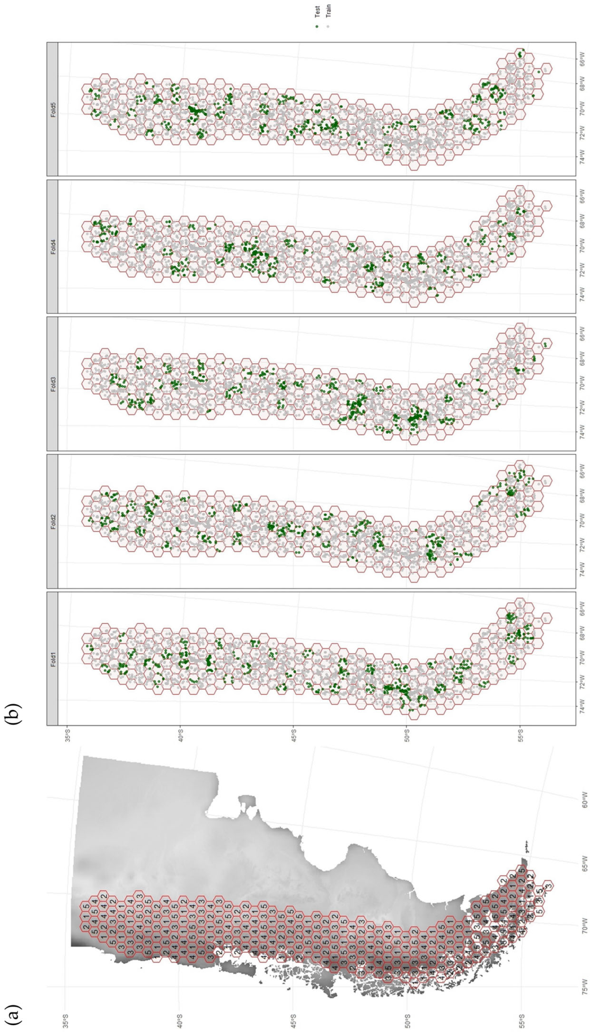
2.4. Model Calibration and Evaluation

Spatial data, such as species and climate data, are often spatially autocorrelated [66,67]. Consequently, when spatial dependence is present in a dataset, spatial (or block) cross-validation is recommended [68]. We performed spatial cross-validation using the R package “blockCV” (version 3.1.5) [69]. For 5-fold cross-validation, the data is initially partitioned into spatial blocks of a predefined size, and each block is randomly assigned to one of five folds (k = 5). The model is then trained on four folds (k - 1) and evaluated on the remaining fold. This procedure is repeated five times, ensuring that each fold serves as both a training and a testing set. To determine an appropriate block size, we initially used the function “cv_spatial_autocor” to calculate the spatial autocorrelation of our species data. Spatial autocorrelation differed slightly between the two datasets (29.6 km for the point dataset and 24.4 km for the raster dataset). Therefore, we opted for a larger block size of 50 km to minimise potential autocorrelation effects and to ensure comparability between the two datasets. The spatial arrangement of the hexagonal blocks is displayed in the Appendix A (Figure A1). To validate the models, we used threshold-independent metrics such as AUC and overall accuracy, as well as threshold-dependent metrics like the True Skill Statistic (TSS), using the maximum sensitivity plus specificity threshold, for the RF classification approach. For the RF regression approach, the root mean square error (RMSE) and the coefficient of determination (R2) were used as validation metrics. In addition to evaluating model performance on the cross-validation splits, we also assessed the models’ hyperparameters. We evaluated models with different numbers of variables considered at each split (mtry: 2, 3, 4) and varying numbers of trees (ntree: 100, 300, 500). Through hyperparameter tuning in combination with spatial cross-validation, we were able to identify the optimal model while minimising the risk of spatial overfitting. The model with the highest average AUC resp. R2 was selected and subsequently used to predict the potential current and future distribution of N. pumilio across the entire dataset.

3. Results

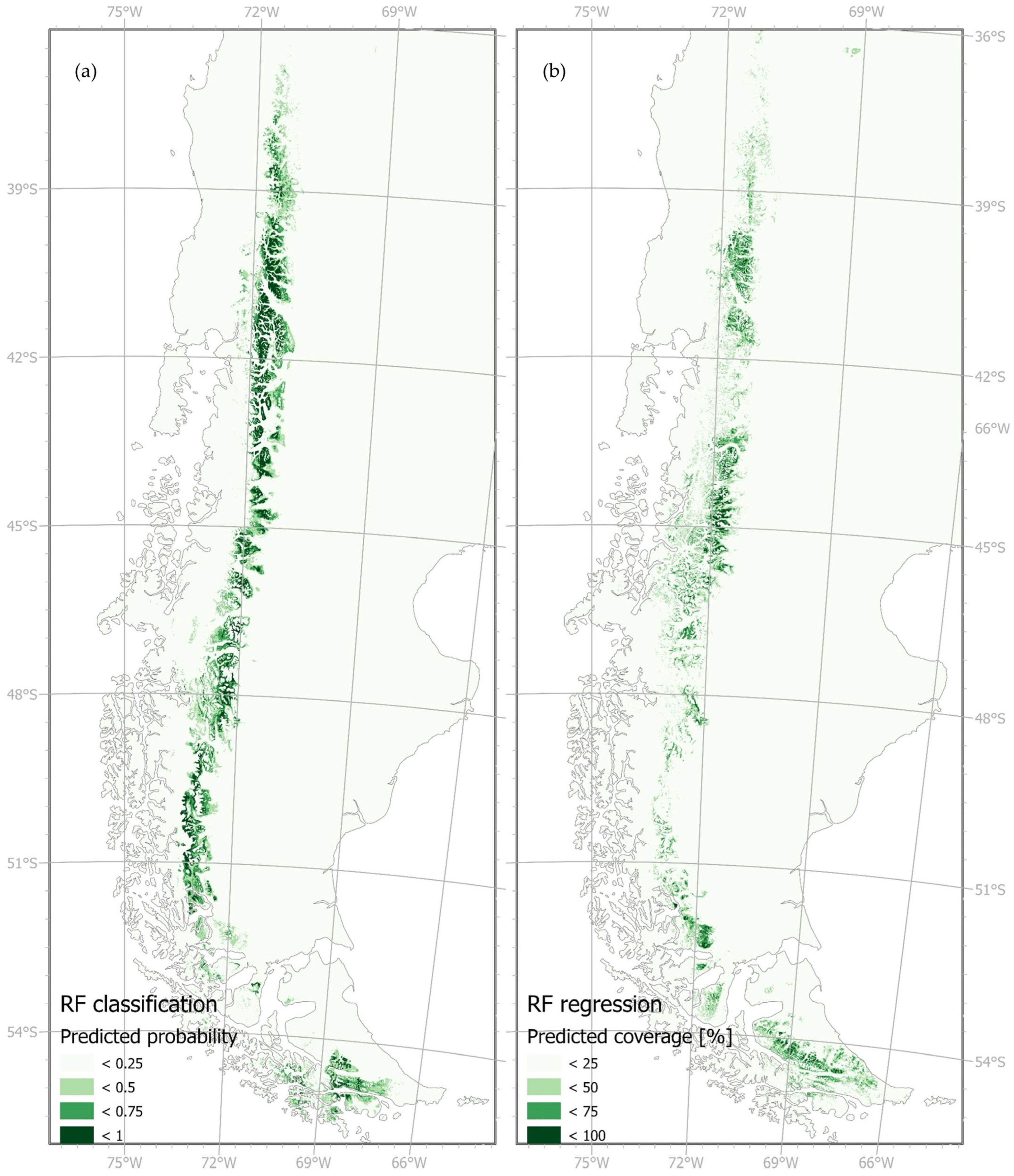
3.1. Current Distribution Range of N. pumilio

The optimal model for predicting the current distribution of N. pumilio was identified using 5-fold spatial cross-validation. The cross-validation results for both models are presented in Table A1 and Table A2 in the Appendix A. Model quality was assessed based on the mean validation metrics across all five folds (for the RF classification model, the optimal model was selected based on the highest AUC; for the RF regression model, selection was based on the highest R2). For the RF classification model, the best-performing model, with hyperparameters mtry = 2 and ntree = 500, achieved the highest mean AUC of 0.9279 (±0.0257, 95% confidence interval (CI): 0.8960–0.9599), an overall accuracy of 0.8466 (±0.0537, 95% CI: 0.7799–0.9132), and a TSS of 0.6148 (±0.1582, 95% CI: 0.4183–0.8112). The final model was subsequently trained using these hyperparameters on the entire dataset. For the RF regression model, the highest mean R2 determined by spatial cross-validation was 0.3933 (±0.0409, 95% CI: 0.3425–0.4441), also indicating mtry = 2 and ntree = 500 as the optimal hyperparameters. The models trained with the optimal hyperparameters and on the complete datasets were then used for variable importance analysis as well as for spatial predictions of current and future distributions.
Bioclimatic variables bio 8 (mean daily mean air temperature of the wettest quarter) and bio 19 (mean monthly precipitation amount of the coldest quarter) emerged as the most influential predictors for model accuracy of the RF classification model (Accuracy Importance ranking, from most to least important bioclimatic variable: bio 8 (mean daily mean air temperatures of the wettest quarter), bio 19 (mean monthly precipitation amount of the coldest quarter), bio 15 (precipitation seasonality), bio 17 (mean monthly precipitation amount of the driest quarter), bio 4 (temperature seasonality), bio 10 (mean daily mean air temperatures of the warmest quarter), bio 18 (mean monthly precipitation amount of the warmest quarter), and bio 11 (mean daily mean air temperatures of the coldest quarter)). Additionally, Gini Importance was calculated to assess the most frequently used variables for decision at nodes, with bio 11 (mean daily mean air temperatures of the coldest quarter) and bio 8 (mean daily mean air temperatures of the wettest quarter) emerging as the primary split criteria for the RF classification model (Gini Importance ranking: bio 11, bio 17, bio 8, bio 10, bio 18, bio 19, bio 4, bio 15). While a temperature variable was the most important predictor in the RF classification model, precipitation-related variables, particularly bio 15 (precipitation seasonality) and bio 19 (mean monthly precipitation amount of the coldest quarter), played a dominant role in the RF regression model (Accuracy Importance ranking: bio 15, bio 19, bio 4, bio 11, bio 10, bio 8, bio 18, bio 17). Gini Importance analysis for the RF regression model indicated that bio 11 (mean daily mean air temperatures of the coldest quarter) was the most critical variable for splits, followed by bio 15 (precipitation seasonality) (Gini Importance ranking: bio 11, bio 15, bio 8, bio 18, bio 4, bio 10, bio 19, bio 17).
A RF model consists of multiple individual decision trees, making it challenging to interpret the specific thresholds used at each node. However, the extraction of partial dependence plots (PDP) for individual variables allows for an interpretation of the influence of specific bioclimatic predictors within the RF model. We employed the “partialPlot” function from the “randomForest” R package (version 4.7-1.2, [70]) to assess the influence of the most important variable in each model. The resulting PDPs are presented in Figure 2a,c. For the RF classification model, the x-axis displays the values of the bioclimatic variable bio 8 (mean daily mean air temperatures of the wettest quarter), while the y-axis represents the predicted probability for class 1 (i.e., presence of N. pumilio). At low temperatures in the wettest quarter (below −5 °C), the predicted probability of occurrence is high, clearly decreasing towards 5 °C and remaining consistently low above this threshold. This indicates that the model predicts the presence of N. pumilio primarily in colder environments during the wettest quarter. In the RF regression model, the x-axis shows the values of bio 15 (precipitation seasonality), and the y-axis represents the predicted cover values of N. pumilio. The plot reveals greater variability, but cover values are relatively high in areas with moderate precipitation seasonality (0% to 30%). However, there is a marked decline in predicted cover values in regions with high precipitation seasonality (70% to 100%). Two key assumptions emerge: cover values are greater in areas with lower precipitation seasonality, suggesting that N. pumilio prefers regions with more stable precipitation patterns and the species is less likely to occur in areas with highly variable precipitation, e.g., with phases of drought.
These effects are also evident in the SHAP summary (bee swarm) plots, created using the “fastshap” R package (version 0.1.1) [71]. SHAP (Shapley Additive Explanation) analysis, which originates from cooperative game theory, provides a comprehensive overview of the contribution of each predictor to the model outcome (see Figure 2b,d) [72]. In the RF classification model, the influence of temperature variables is consistent: high temperatures have a negative effect on the model (indicating absence), while low temperatures have a positive effect (indicating presence). In the RF regression model, the influence of temperature variables varies. For bio 8 (mean daily mean air temperatures of the wettest quarter) and bio 11 (mean daily mean air temperatures of the coldest quarter), low temperatures also have a positive influence on the model outcome (higher cover values), whereas this effect is reversed for bio 10. For bio 10 (mean temperature of the warmest quarter), low temperatures result in a decrease in cover values, while intermediate temperatures lead to an increase. Bio 11, particularly in the RF regression model, exhibits a wide range, indicating a strong influence on both models. This is further supported by the variable importance analysis, which identifies bio 11 as the most important splitting criterion at nodes based on Gini importance. The pattern for precipitation variables is less distinct; however, the trend is similar in both models: low to medium precipitation totals have a positive effect on the model. A similar trend can also be observed for seasonality variables bio 4 (temperature seasonality) and bio 15 (precipitation seasonality). Low to moderate values of these variables are associated with species occurrence, whereas very low or very high values result in a reduced probability of presence and lower cover values.
The spatial predictions of the two models revealed a more compact distribution in the RF classification model, with a slightly broader extent towards the west and east for the RF regression model. The binary RF classification model predicted a northern extent of up to 36.35° S and a southern extent of 55.45° S, whereas the RF regression model extended from 35.24° S to 55.24° S (Figure 3). In the southern regions, including Tierra del Fuego, the RF regression model depicted a more homogeneous distribution. IGTA points were lacking in this area resulting in gaps in the predicted occurrence. While the RF classification model tended to overpredict in unvegetated summit regions and glaciated areas, the RF regression model provided a more fine-grained representation, capturing vegetated valleys more accurately. When compared with a digital surface model (DSM, ALOS Global Digital Surface Model, 30 m), it was evident that the RF classification model predicted suitable climatic conditions in higher (unvegetated) areas as distribution areas, while in the RF regression model they were omitted. The described small-scale differences between the models are illustrated in Figure 4.
To further validate the spatial predictions of the models, we conducted two additional comparisons. First, we performed a visual comparison of the model outputs with independent data provided by the Argentinian forestry authority (Secretaría de Ambiente y Desarrollo Sustentable de la Nación, [73]). Second, we compared the elevation of high-altitude raster cells from both models with reported treeline elevations from 48 plots across 13 locations, as published by Lara et al. (2005) [74]. Figure 5 presents the visual comparison between the raster outputs of the models and the N. pumilio forest polygons. The RF classification model shows slightly more deviation and tends to extend beyond the polygon boundaries, while the RF regression model closely matches the reference polygons. Table 2 compares the treeline elevations from on-site measurements [74] with the elevations of the highest raster cells predicted by the models (based on a DSM resampled to 1 km), which are intended to approximate the treeline position. To identify these treeline raster cells, a threshold is required. Based on the range of definitions compiled in the literature, the treeline can be defined as the elevation at which tree canopy cover declines to approximately 30%, representing the uppermost margin of closed forest [18]. Accordingly, we applied a threshold of 30% (resp. 0.3 for RF classification) to the model outputs. In the RF classification model, treeline elevations are, in some cases, significantly higher than the treeline elevations measured on site. However, in the southern regions, the predicted treeline aligns well with the literature. In contrast, the RF regression model predicts treeline elevations that are only slightly higher in the north and overall correspond closely to the reported values.

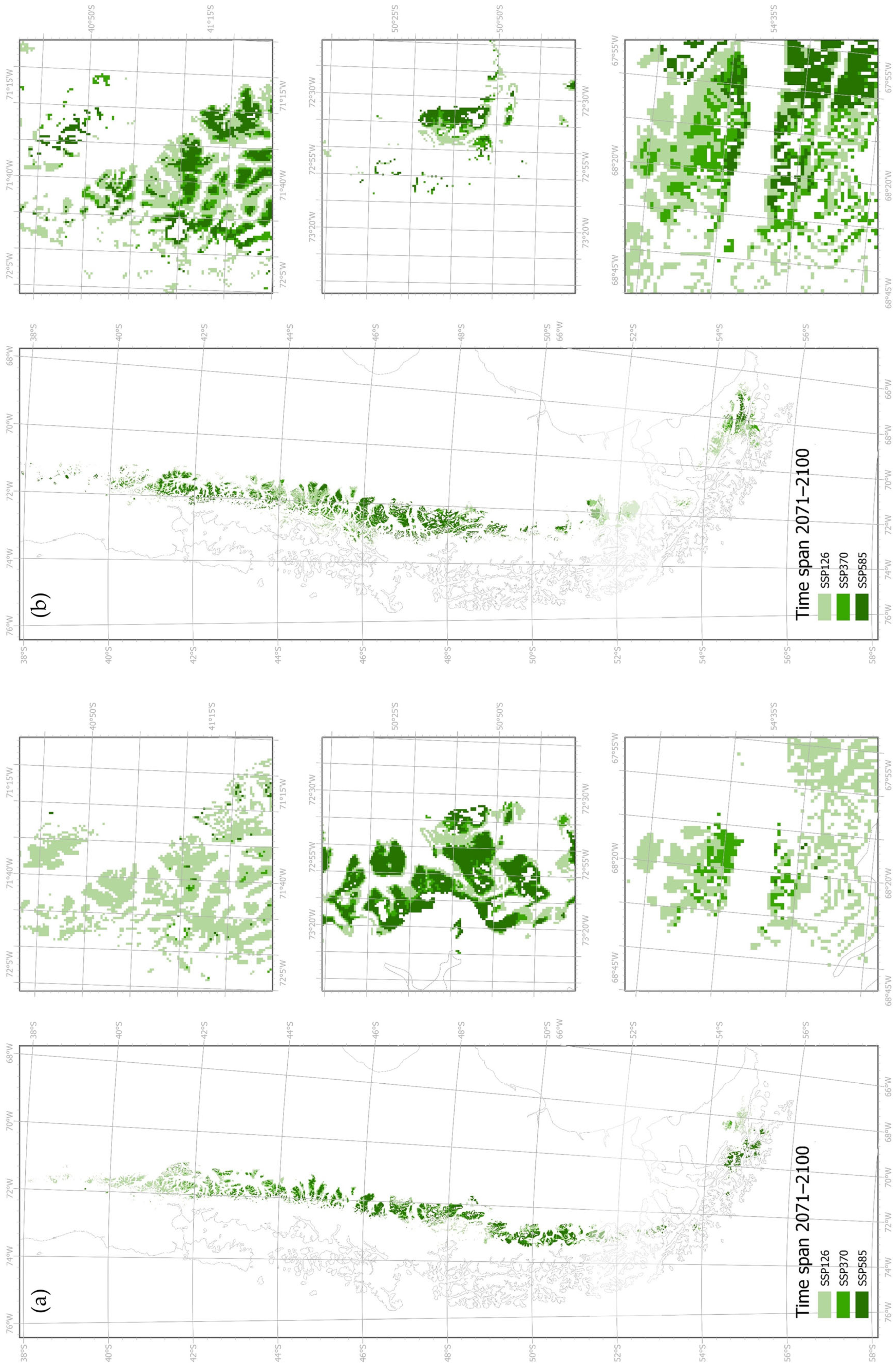
3.2. Future Distribution Range of N. pumilio

Using CMIP6 data provided by CHELSA for the SSP scenarios, we predicted the potential future distribution of N. pumilio with both models. Predictions were generated for the SSP126, SSP370, and SSP585 scenarios for two future periods: 2041–2070 and 2071–2100. Figure 6a,b illustrate the potential distribution of N. pumilio for 2041–2070, while Figure A2a,b in the Appendix A depict projections for 2071–2100. For the RF classification model, the SSP scenarios for the period 2041–2070 already indicate a potential shift in distribution towards currently unvegetated summit areas. This upward shift to higher elevations becomes more pronounced with increasingly severe scenarios (SSP370, SSP585). Simultaneously, there is a progressive decline in occurrences throughout the northern part of the species’ range, and a slight decrease in the southernmost distribution areas. Additionally, the occurrences are predicted to shift towards the more humid western regions. These trends become even more marked in the period from 2071 to 2100. During this later time span, a decrease in occurrence area is evident, particularly at lower elevations, resulting in an overall stronger decline in the north. Both models consistently indicate a reduction in occurrences in northern regions. However, in contrast to the RF classification model, the RF regression model suggests that N. pumilio is more likely to persist at higher elevations in the north, and that the decline in occurrences in the southernmost parts of the range is less pronounced. The total decreases in distribution area and the westward shift are less marked in the RF regression model, with eastern occurrences more likely to remain stable. Nevertheless, the trend of occurrences shifting towards higher elevations is observed in both models, and this trend intensifies with the severity of the scenario and over time. While the RF classification model predicts an expansion into higher, currently snow- and ice-covered areas of the Southern Patagonian Icefield, the RF regression model forecasts a decline in occurrences in this region. Despite this, under the scenarios for 2071–2100, the RF regression model also projects a reduction in occurrences at lower elevations, which ultimately results in a net decrease in the total distribution area of the species. Thus, both modelling approaches reveal potential changes in the distribution of N. pumilio under future climate scenarios, particularly in lowland and northern areas, but they differ slightly with respect to the potential persistence of the species at higher elevations in the north and in the southern part of its range.
To assess treeline shifts in numbers, we again refer to the comparison of treeline elevations at the 13 locations. In Table 3, we compare the elevation of the highest raster cells at the treeline sites under current climatic conditions and under the SSP scenarios for the period 2041–2070 (for the time span 2071–2100, please refer to Table A3 in the Appendix A). Even under current climatic conditions, no occurrence was recorded at the northernmost site (site no. 1), and this remains the case across all scenarios. The predicted decline in the northern distribution range continues, with no remaining occurrences at the second site under the SSP370 scenario. Overall, the estimated treeline elevations in the RF classification model are generally higher than those predicted by the RF regression model. As climate scenarios progress, a general upward shift in treeline elevation is observed, with a few exceptions where treeline elevation either stagnates, mainly due to already having reached the highest local topography, or shows a slight decrease. These trends are also evident in the period 2071–2100, with even higher treeline elevations in most cases, or occasional decreases due to an overall loss of suitable area in the region.

4. Discussion

The treeline species Nothofagus pumilio is highly sensitive to climate variations, as reflected in its radial growth patterns and seedling establishment above the treeline. Consequently, research into the species’ treeline dynamics in response to climate change has already gained some attention. Many studies have examined growth variations using dendrochronology, providing insights into the species’ response to climate variations, mostly related to expressions in ENSO, PDO, and AAO/SAM over the past century [22,25,26]. Other research has focused on seedling establishment [23,24,75] or assessed the quantity and quality of N. pumilio seeds [17,75,76]. However, large-scale Species Distribution Modelling (SDM) approaches investigating the current and future development of the species are lacking. In this study, we calculated two Random Forest (RF) models using a binary and a continuous species dataset to model the current and future potential distribution of the species.
Both models, RF classification and RF regression, achieved reasonable results and good performance values. The RF classification model achieved an AUC of 0.93 (95% CI: 0.90–0.96), whereas the RF regression model explained R2 = 0.39 (95% CI: 0.34–0.44) of the variance. This discrepancy is primarily due to the greater noise and structural complexity inherent in the continuous response variable, as well as the inherently stricter nature of R2 as a performance metric. The use of spatially blocked cross-validation further amplifies this issue, because the model must extrapolate beyond clusters of spatially autocorrelated observations along the treeline. Consequently, an R2 of around 0.4 can already be considered good performance in ecological regression tasks. The RF algorithm is well-suited for this study due to its strong predictive power and, more importantly, its applicability to both datasets, enabling direct comparability. Moreover, RF is a well-established algorithm that facilitates comparisons between different modelling approaches within the field of SDM [60,77]. While binary approaches are mainly used in SDM, the use of a continuous target variable generated from remote sensing, rather than the generation of abiotic predictors, is still a novel approach. The continuous data were derived from 20 m raster cells, with coverage aggregated to the target resolution of 1 km. While the binary variable contains only information on presence or absence, the continuous data reflect additional influences from land cover and species composition, which affect cover values and provide ecologically meaningful information. Other studies investigating topographic complex regions have already discussed the loss of knowledge due to the use of binary data at 1 km spatial resolution [56]. Here, we demonstrated an information gain using 1 km resolution data while incorporating continuous variables.
It should be noted that the scales of the modelling approaches (RF classification and RF regression) differ. However, we compare the model outputs, predicted probability and predicted cover values, on the basis that both a low predicted probability and a low cover value indicate largely unsuitable bioclimatic conditions, whereas high probability values and cover values point to suitable conditions. Nevertheless, it is important to acknowledge that a probability of 0.01 reflects only a very low likelihood of the species occurring at all, whereas 1% cover implies the species is present, albeit in low abundance. Although the models differ in their spatial predictions and variable importance, the correlation between predicted probability and cover values is relatively high, with a Pearson’s r of 0.6. We therefore treat the two metrics as complementary, not interchangeable, and interpret model outputs jointly.

4.1. Current Distribution Range of N. pumilio

Differences between the two models were apparent across all analyses. In terms of spatial prediction, the RF regression model captured fine-scale details more accurately and was less prone to overprediction at high elevations. Additionally, the key predictors for the RF models varied. While a temperature variable had the highest importance (Accuracy Importance) in the RF classification model, precipitation variables had the highest importance in the RF regression model. Although the SHAP plots differ slightly in their expression between the models, the suitable bioclimatic conditions for N. pumilio are clearly evident in both. The species benefits from cold winters (bio 11, mean daily mean air temperatures of the coldest quarter) combined with moderate levels of precipitation, presumably in the form of protective snow cover (bio 19, mean monthly precipitation amount of the coldest quarter), and cool summers (moderate values of bio 10 (mean daily mean air temperatures of the warmest quarter)). Moreover, N. pumilio tends to occur in regions with sufficient overall precipitation and low precipitation seasonality, reflected by low to medium values for bio 17 (mean monthly precipitation amount of the driest quarter), bio 18 (mean monthly precipitation amount of the warmest quarter), and bio 15 (precipitation seasonality). Extreme heat or pronounced drought conditions inhibit the species’ presence. Both temperature and precipitation seasonality are low, indicating that the species does not occur in areas characterised by extreme temperature fluctuations or erratic precipitation patterns, such as extended dry periods. The orophilous species N. pumilio is particularly adapted to the harsh climatic conditions of high mountain ecosystems. The species shows high phenotypic plasticity. While occurring at lower elevations as an erect tree up to a height of 35 m, it shows krummholz growth forms at the treeline [78]. As a deciduous species, it reduces transpiration in the months when frost-drought can be a problem [79]. Heat deficiency is considered to be the most important site factor for treeline formation worldwide. The treeline of N. pumilio follows an isotherm of 6.6 °C [19]. The influence of temperature was shown in the RF classification model by the high importance of bio 8 (mean daily air temperature of the wettest quarter), by the fact that the variable bio 11 (mean daily mean air temperatures of the coldest quarter) has a very important influence on the decisions at the nodes of both models (Gini Importance), and in the SHAP plots. However, when modelling a species in high mountains, the influence of elevation can also be represented by temperature variables. In the SHAP plot of the RF classification model, only very high temperature values in the warmest quarter (bio 10) result in a reduction in predicted probability. In contrast, in the RF regression model, very low temperatures during the warmest quarter lead to a decrease in predicted cover values. This difference is also reflected in the spatial predictions, with the RF classification model showing slight overprediction in summit regions. However, high temperatures during the warmest quarter can also lead to drought events, particularly in high mountain ecosystems where insolation and consequently evapotranspiration is very high. Authors analysing the sensitivity of N. pumilio to climate change using changes in tree rings have found a correlation with precipitation regimes in addition to temperatures. The species occurs in humid to arid regions and is well adapted to medium to low precipitation sums that occur at high elevations due to advective precipitation. This is also shown by its occurrence as far as the arid east, where it sometimes forms two treelines: an alpine treeline and a xeric treeline towards the arid steppes [80]. Very low values for precipitation variables (bio 17, 18 and 19) and precipitation seasonality (bio 15) define the limits in the core range and the eastern boundary of the species. However, particularly in northern Patagonia, increasingly low precipitation during the spring and summer months negatively affects tree growth [22,81]. In more southerly regions, high spring precipitation is primarily associated with prolonged snow cover, leading to a shortened growing season, which in turn also hinders tree growth [22,82,83]. Between 1900 and 2020, tree growth was found to correlate most strongly with rising temperatures on mesic sites, followed by wetter sites, while growth rates declined on drier sites [25]. Some authors state that all treelines in southern South America have experienced a negative growth trend due to drought since the 1980s and even suggest that the limitation at the treeline has changed from cold-limited to drought-limited [26,84]. Our results of the RF regression model seem plausible in this context, as the precipitation variables bio 15 (precipitation seasonality) and bio 19 (mean monthly precipitation of the coldest quarter) played an important role. Both variables reflect annual precipitation distribution patterns. Bio 15 suggests that N. pumilio is unlikely to occur in regions with high precipitation seasonality, which may be associated with periods of drought. Bio 19, on the other hand, may be linked to precipitation in the form of snow, the resulting snow cover, and water availability following thaw.

4.2. Future Distribution Range of N. pumilio

Abrupt treelines respond less to global warming than diffuse treelines, primarily due to higher seedling mortality outside the protecting forest stand climate [14]. The emergence and establishment of seedlings represent the most critical life stage for trees at the treeline, with the availability of species-specific safe sites being the basic precondition for seedling recruitment [85,86]. Seed production, fruit dispersal, seed viability, and seedling establishment all decline with increasing elevation [17]. Higher temperatures and an extension of the growing season can thus facilitate seedling emergence and survival [19,23,24,75,81], a precondition for a future treeline advance. However, the comparatively slow advance or persistence of the treeline in the southern Andes is also linked to multi-faceted interactions with edaphic, topographic, biotic, and other factors, including the development of alpine mats [24,28]. Demographic constraints across different life stages have been highlighted in previous studies examining the relationship between climate change and tree habitats. As treelines shift to higher elevations, trees are exposed to new climate–habitat interactions, and different life stages may respond in distinct ways [87,88]. For instance, tree fertility is primarily influenced by temperature, whereas seedling establishment depends more heavily on moisture availability and soil water content [87]. In fact, seedling survival declines with increasing drought at both high and low elevations, although at some high elevation stands this effect can be mitigated by spring snow cover [75]. A deterioration in growth conditions due to drought is also predicted for adult trees at lower elevations as well as at the treeline, based on studies of radial growth patterns [26,84,89]. However, even if temperature and precipitation conditions are favourable for seedling establishment, local factors such as steep topography and the absence of herbaceous vegetation can inhibit treeline advance [24,28]. While this study focuses on assessing the effects of key climatic drivers on the treeline, future modelling efforts should consider incorporating additional variables such as topography, wind exposure, soil characteristics, and vegetation cover.
The use of CMIP6 SSP scenarios from CHELSA showed an advance to higher elevations in both models, as indicated by spatial predictions and treeline elevation estimates derived from a digital surface model (DSM). The scenarios are based on global circulation models and CO2 concentration estimates. It should be noted that less periodic variations caused by different phases of ENSO, PDO, and AAO/SAM cannot be fully modelled in the scenarios [90]. While the RF classification model showed a significant decrease in the northern range, lower cover values of the RF regression model remained at higher elevations. The result that N. pumilio occurrences decreased at lower elevations is consistent with previous findings [75], highlighting a decrease in the number of seedlings and a reduction in survival at lower-elevated sites. A review study modelling biome-level changes predicts a reduction in area with suitable climatic conditions for temperate deciduous forests of approximately 30% under the RCP8.5 scenario for the period 2040–2070 [16]. Our results seem congruent with these findings, whereas the RF classification model predicts a greater decline than the RF regression model. In particular, the RF classification model predicted a shift towards the wetter western region. It will be necessary to investigate the future competitive relationships with dominant tree species in this area (e.g., N. betuloides). In summary, precipitation conditions/drought stress will play a significant role in future competitive relationships and successful regeneration of Nothofagus species in the southern Andes.

5. Conclusions

To our knowledge, this is the first SDM study that models the current and future distribution of N. pumilio across its entire distribution range in the southern Andes. Even though the distribution range encompasses two extreme climatic gradients, both models were able to comprehensively predict the current potential distribution and its future development. The direct comparison of model approaches highlighted major differences in the model results and the advantages of using more complex, continuous data. Continuous data can provide better insights into suitable bioclimatic conditions for N. pumilio occurrence leading to more detailed spatial predictions and meaningful predictors based on variable importance. In contrast to presence–absence data, which can only take values of 0 or 1, continuous cover values can reflect subtle or unknown effects of land cover, topography, and species composition, thereby providing model results of greater ecological value. However, we acknowledge that remote sensing data across a large geographic extent are rarely available, difficult to obtain in very high resolution, and may still contain gaps that introduce bias. Climatic parameters represent the principal limiting factors at the alpine treeline, and bioclimatic variables have already proven effective in capturing the climatic conditions at the treeline of the southern Andes. It will be of great interest to further model the conditions at the treeline with more complex abiotic predictors, like topography, wind and soil variables as well as to embed biotic and anthropogenic variables to model the influences of vegetation composition, fire, grazing, and forestry.

Author Contributions

Conceptualization, M.W., J.B., J.O., U.S., J.W. and M.B.; methodology, M.W., J.O., J.W. and M.B.; validation, M.W., J.O. and M.B.; formal analysis, M.W.; investigation, M.W.; data curation, M.W.; writing—original draft preparation, M.W.; writing—review and editing, M.W., J.B., J.O., U.S. and M.B.; visualisation, M.W.; supervision, J.B. and U.S. All authors have read and agreed to the published version of the manuscript.

Funding

This research received no external funding.

Data Availability Statement

The species input data used in this study are online available at the free data provider of University of Hamburg: http://doi.org/10.25592/uhhfdm.16239, accessed on 7 June 2025.

Conflicts of Interest

The authors declare no conflicts of interest.

Appendix A

Appendix A.1

Figure A1. (a) Hexagonal spatial blocks with the allocation of folds (1–5), created using the “blockCV” R package, and (b) the five folds showing test data points (dark green) and training data points (grey) for the Random Forest classification model.
Forests 16 01211 g0a1

Appendix A.2

Figure A2. Potential future distribution of Nothofagus pumilio modelled by (a) the Random Forest classification and (b) RF regression model using CMIP6 SSP Scenarios for CHELSA Bioclim variables for the time span of 2071 to 2100.
Forests 16 01211 g0a2

Appendix A.3

Table A1. Results of the 5-fold spatial cross-validation of the Random Forest classification model. The table presents the mean values across all five models for the various hyperparameter settings (45 models in total). The hyperparameter setting for the final model, highlighted in bold, was selected based on the highest mean AUC.
No.mtryntreeAUC MeanAUC 95% CI 1Acc. MeanAcc. 95% CI 1TSS MeanTSS 95% CI 1
121000.92700.8908–0.96320.84600.7782–0.91390.61250.4169–0.8081
231000.92040.8785–0.96230.84070.7803–0.90110.59680.4164–0.7772
341000.91920.8821–0.95640.84540.7761–0.91470.61060.4025–0.8187
423000.92680.8943–0.95920.84410.7767–0.91150.60530.4063–0.8043
533000.92370.8884–0.95900.84730.7827–0.91180.61630.4212–0.8114
643000.92280.8898–0.95570.84610.7831–0.90920.61270.4265–0.7988
725000.92790.8960–0.95990.84660.7799–0.91320.61480.4183–0.8112
835000.92330.8881–0.95850.84380.7765–0.91110.60250.4015–0.8035
945000.92240.8837–0.96100.84290.7756–0.91020.60500.4082–0.8019
1 Confidence intervals.
Table A2. Results of the 5-fold spatial cross-validation of the Random Forest regression model. Hyperparameter for the final model, highlighted in bold, were selected based on the highest mean R2.
No.mtryntreeR2 Mean95% CI 1
121000.39100.3419–0.4400
231000.38680.3366–0.4369
341000.38350.3323–0.4348
423000.39330.3432–0.4433
533000.38920.3378–0.4407
643000.38730.3362–0.4384
725000.39330.3425–0.4441
835000.38980.3386–0.4410
945000.38690.3357–0.4381
1 Confidence intervals.
Table A3. Treeline elevation estimates based on the highest raster cells from the model outputs (Random Forest classification and RF regression) under current climatic conditions and SSP scenarios for the future period 2071–2100. NA = not available (no data recorded).
CoordinatesTreeline Elevation [m] Current ClimateTreeline Elevation [m] SSP126 (2071–2100)Treeline Elevation [m] SSP370 (2071–2100)Treeline Elevation [m] SSP585 (2071–2100)
XYRF Class.RF Reg.RF Class.RF Reg.RF Class.RF Reg.RF Class.RF Reg.
−71.00−35.36NANANANANANANANA
−71.11−37.27198819492328NANANANA2530
−71.33−38.4218541789207117001780187124602035
−72.15−40.4215911437167916362026197120262026
−72.19−41.4815001201155515101917174319171730
71.45−43.0718391440195515452059195520592059
−71.42−44.3913201216170315951952159319521427
−72.24−47.1213611197143913461742165119011840
−72.30−48.3015221074139910981578117116981340
−72.54−50.571176956131710001457122915371287
−71.00−53.00543560592728NANANANA
−68.45−54.17544520648616615757NANA
−67.30−54.57610610609614NA614NA614

References

  1. Holtmeier, F.-K.; Broll, G. Treeline Research—From the Roots of the Past to Present Time. A Review. Forests 2020, 11, 38. [Google Scholar] [CrossRef]
  2. Schickhoff, U.; Bobrowski, M.; Mal, S.; Schwab, N.; Singh, R.B. The World’s Mountains in the Anthropocene. In Mountain Landscapes in Transition; Schickhoff, U., Singh, R.B., Mal, S., Eds.; Springer International Publishing: Cham, Switzerland, 2022; pp. 1–144. ISBN 978-3-030-70237-3. [Google Scholar]
  3. Körner, C. Climatic Controls of the Global High Elevation Treelines. In Encyclopedia of the World’s Biomes; Elsevier: Amsterdam, The Netherlands, 2020; pp. 275–281. ISBN 9780128160978. [Google Scholar]
  4. Paulsen, J.; Körner, C. A climate-based model to predict potential treeline position around the globe. Alp. Bot. 2014, 124, 1–12. [Google Scholar] [CrossRef]
  5. Qiu, J.; Feng, S.; Yuan, W. Upward-moving mountain treelines: An indicator of changing climate. Glob. Change Biol. 2023, 29, 6832–6833. [Google Scholar] [CrossRef]
  6. Schickhoff, U.; Bobrowski, M.; Böhner, J.; Bürzle, B.; Chaudhary, R.P.; Gerlitz, L.; Heyken, H.; Lange, J.; Müller, M.; Scholten, T.; et al. Do Himalayan treelines respond to recent climate change? An evaluation of sensitivity indicators. Earth Syst. Dynam. 2015, 6, 245–265. [Google Scholar] [CrossRef]
  7. Schickhoff, U.; Bobrowski, M.; Böhner, J.; Bürzle, B.; Chaudhary, R.P.; Müller, M.; Scholten, T.; Schwab, N.; Weidinger, J. The Treeline Ecotone in Rolwaling Himal, Nepal: Pattern-Process Relationships and Treeline Shift Potential. In Ecology of Himalayan Treeline Ecotone; Singh, S.P., Reshi, Z.A., Joshi, R., Eds.; Springer Nature: Singapore, 2023; pp. 95–145. ISBN 978-981-19-4475-8. [Google Scholar]
  8. Treml, V.; Veblen, T.T. Does tree growth sensitivity to warming trends vary according to treeline form? J. Biogeogr. 2017, 44, 1469–1480. [Google Scholar] [CrossRef]
  9. Harsch, M.A.; Hulme, P.E.; McGlone, M.S.; Duncan, R.P. Are treelines advancing? A global meta-analysis of treeline response to climate warming. Ecol. Lett. 2009, 12, 1040–1049. [Google Scholar] [CrossRef]
  10. Hansson, A.; Dargusch, P.; Shulmeister, J. A review of modern treeline migration, the factors controlling it and the implications for carbon storage. J. Mt. Sci. 2021, 18, 291–306. [Google Scholar] [CrossRef]
  11. Hansson, A.; Shulmeister, J.; Dargusch, P.; Hill, G. A review of factors controlling Southern Hemisphere treelines and the implications of climate change on future treeline dynamics. Agric. For. Meteorol. 2023, 332, 109375. [Google Scholar] [CrossRef]
  12. Lu, X.; Liang, E.; Wang, Y.; Babst, F.; Camarero, J.J. Mountain treelines climb slowly despite rapid climate warming. Glob. Ecol. Biogeogr. 2021, 30, 305–315. [Google Scholar] [CrossRef]
  13. Harsch, M.A.; Bader, M.Y. Treeline form—A potential key to understanding treeline dynamics. Glob. Ecol. Biogeogr. 2011, 20, 582–596. [Google Scholar] [CrossRef]
  14. Bader, M.Y.; Llambí, L.D.; Case, B.S.; Buckley, H.L.; Toivonen, J.M.; Camarero, J.J.; Cairns, D.M.; Brown, C.D.; Wiegand, T.; Resler, L.M. A global framework for linking alpine-treeline ecotone patterns to underlying processes. Ecography 2021, 44, 265–292. [Google Scholar] [CrossRef]
  15. Körner, C. Alpine Treelines; Springer: Basel, Switzerland, 2012; ISBN 978-3-0348-0395-3. [Google Scholar]
  16. Tovar, C.; Carril, A.F.; Gutiérrez, A.G.; Ahrends, A.; Fita, L.; Zaninelli, P.; Flombaum, P.; Abarzúa, A.M.; Alarcón, D.; Aschero, V.; et al. Understanding climate change impacts on biome and plant distributions in the Andes: Challenges and opportunities. J. Biogeogr. 2022, 49, 1420–1442. [Google Scholar] [CrossRef] [PubMed]
  17. Cuevas, J.G. Tree recruitment at the Nothofagus pumilio alpine timberline in Tierra del Fuego, Chile. J. Ecol. 2000, 88, 840–855. [Google Scholar] [CrossRef]
  18. Holtmeier, F.-K. Mountain Timberlines: Ecology, Patchiness, and Dynamics; Springer: Dordrecht, The Netherlands, 2009; ISBN 978-1-4020-9704-1. [Google Scholar]
  19. Fajardo, A.; Piper, F.I. An experimental approach to explain the southern Andes elevational treeline. Am. J. Bot. 2014, 101, 788–795. [Google Scholar] [CrossRef] [PubMed]
  20. Bozkurt, D.; Rojas, M.; Boisier, J.P.; Valdivieso, J. Projected hydroclimate changes over Andean basins in central Chile from downscaled CMIP5 models under the low and high emission scenarios. Clim. Change 2018, 150, 131–147. [Google Scholar] [CrossRef]
  21. Pessacg, N.; Flaherty, S.; Solman, S.; Pascual, M. Climate change in northern Patagonia: Critical decrease in water resources. Theor. Appl. Clim. 2020, 140, 807–822. [Google Scholar] [CrossRef]
  22. Álvarez, C.; Veblen, T.T.; Christie, D.A.; González-Reyes, Á. Relationships between climate variability and radial growth of Nothofagus pumilio near altitudinal treeline in the Andes of northern Patagonia, Chile. For. Ecol. Manag. 2015, 342, 112–121. [Google Scholar] [CrossRef]
  23. Srur, A.M.; Villalba, R.; Rodríguez-Catón, M.; Amoroso, M.M.; Marcotti, E. Establishment of Nothofagus pumilio at Upper Treelines Across a Precipitation Gradient in the Northern Patagonian Andes. Arct. Antarct. Alp. Res. 2016, 48, 755–766. [Google Scholar] [CrossRef]
  24. Srur, A.M.; Villalba, R.; Rodríguez-Catón, M.; Amoroso, M.M.; Marcotti, E. Climate and Nothofagus pumilio Establishment at Upper Treelines in the Patagonian Andes. Front. Earth Sci. 2018, 6, 57. [Google Scholar] [CrossRef]
  25. Brand, R.; Srur, A.M.; Villalba, R. Contrasting growth trends in Nothofagus pumilio upper-elevation forests induced by climate warming in the Southern Andes. Agric. For. Meteorol. 2022, 323, 109083. [Google Scholar] [CrossRef]
  26. Reiter, E.J.; Weigel, R.; Walentowski, H.; Loguercio, G.A.; Fierke, J.; Winter, A.F.N.; Simon, A.; Kotowska, M.M.; Joelson, N.Z.; Caselli, M.; et al. Climate vulnerability of Nothofagus pumilio, Nothofagus dombeyi and Austrocedrus chilensis in northern Patagonia’s temperate forests. For. Ecol. Manag. 2024, 572, 122261. [Google Scholar] [CrossRef]
  27. Rodriguez-Souilla, J.; Cellini, J.M.; Roig, F.A.; Lencinas, M.V.; Chaves, J.E.; Peri, P.L.; Martínez Pastur, G.J. Climate influence seed production in managed and unmanaged Nothofagus pumilio forests of Southern Patagonia. NZJFS 2024, 54, 1–14. [Google Scholar] [CrossRef]
  28. Pissolito, C. Sucesión Primaria de la Vegetación en Bosques de Nothofagus spp. en los Andes Patagónicos: Patrones Espacio Temporales de Establecimiento de Plantas e Implicancias Para la Restauración. Ph.D. Thesis, Universidad Nacional de Cuyo, Mendoza, Argentina, 2016. [Google Scholar]
  29. Feng, X.; Park, D.S.; Walker, C.; Peterson, A.T.; Merow, C.; Papeş, M. A checklist for maximizing reproducibility of ecological niche models. Nat. Ecol. Evol. 2019, 3, 1382–1395. [Google Scholar] [CrossRef]
  30. Karger, D.N.; Conrad, O.; Böhner, J.; Kawohl, T.; Kreft, H.; Soria-Auza, R.W.; Zimmermann, N.E.; Linder, H.P.; Kessler, M. Climatologies at high resolution for the earth’s land surface areas. Sci. Data 2017, 4, 170122. [Google Scholar] [CrossRef] [PubMed]
  31. Karger, D.N.; Wilson, A.M.; Mahony, C.; Zimmermann, N.E.; Jetz, W. Global daily 1 km land surface precipitation based on cloud cover-informed downscaling. Sci. Data 2021, 8, 307. [Google Scholar] [CrossRef] [PubMed]
  32. Pocock, M.J.O.; Tweddle, J.C.; Savage, J.; Robinson, L.D.; Roy, H.E. The diversity and evolution of ecological and environmental citizen science. PLoS ONE 2017, 12, e0172579. [Google Scholar] [CrossRef] [PubMed]
  33. Aceves-Bueno, E.; Adeleye, A.S.; Feraud, M.; Huang, Y.; Tao, M.; Yang, Y.; Anderson, S.E. The Accuracy of Citizen Science Data: A Quantitative Review. Bull. Ecol. Soc. Am. 2017, 98, 278–290. [Google Scholar] [CrossRef]
  34. Beck, J.; Böller, M.; Erhardt, A.; Schwanghart, W. Spatial bias in the GBIF database and its effect on modeling species’ geographic distributions. Ecol. Inform. 2014, 19, 10–15. [Google Scholar] [CrossRef]
  35. Marcer, A.; Chapman, A.D.; Wieczorek, J.R.; Xavier Picó, F.; Uribe, F.; Waller, J.; Ariño, A.H. Uncertainty matters: Ascertaining where specimens in natural history collections come from and its implications for predicting species distributions. Ecography 2022, 2022, e06025. [Google Scholar] [CrossRef]
  36. Chauvier, Y.; Zimmermann, N.E.; Poggiato, G.; Bystrova, D.; Brun, P.; Thuiller, W. Novel methods to correct for observer and sampling bias in presence-only species distribution models. Glob. Ecol. Biogeogr. 2021, 30, 2312–2325. [Google Scholar] [CrossRef]
  37. Rocchini, D.; Boyd, D.S.; Féret, J.-B.; Foody, G.M.; He, K.S.; Lausch, A.; Nagendra, H.; Wegmann, M.; Pettorelli, N. Satellite remote sensing to monitor species diversity: Potential and pitfalls. Remote Sens. Ecol. Conserv. 2016, 2, 25–36. [Google Scholar] [CrossRef]
  38. Reddy, C.S. Remote sensing of biodiversity: What to measure and monitor from space to species? Biodivers. Conserv. 2021, 30, 2617–2631. [Google Scholar] [CrossRef]
  39. Wang, L.; Diao, C.; Lu, Y. The role of remote sensing in species distribution models: A review. Int. J. Remote Sens. 2025, 46, 661–685. [Google Scholar] [CrossRef]
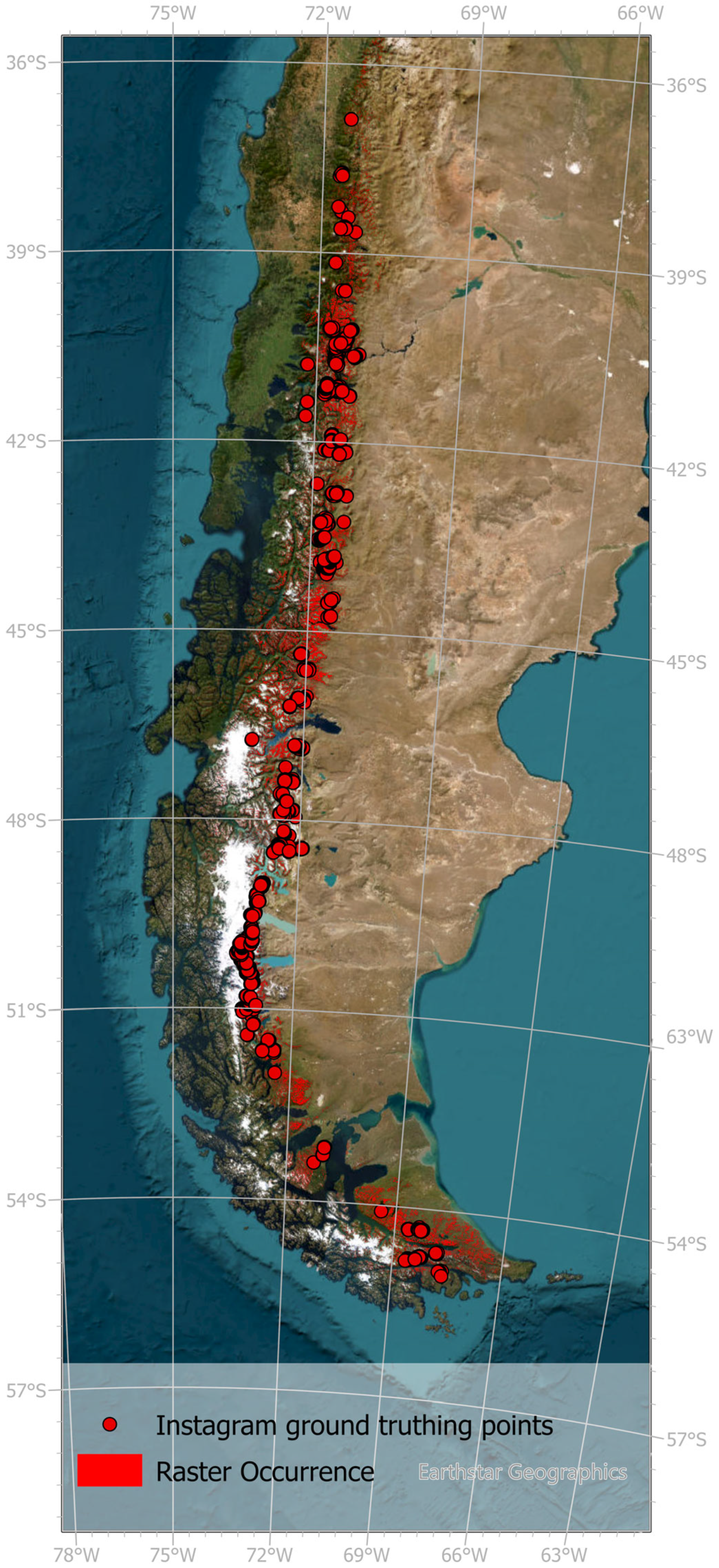
  40. Werner, M.; Weidinger, J.; Böhner, J.; Schickhoff, U.; Bobrowski, M. Instagram data for validating Nothofagus pumilio distribution mapping in the Southern Andes: A novel ground truthing approach. Biogeography 2024, 17, e140606. [Google Scholar] [CrossRef]
  41. Amigo Vázquez, F.J.; Rodríguez Guitián, M.A. Bioclimatic and phytosociological diagnosis of the species of the Nothofagus genus (Nothofagaceae) in South America. IJGR 2011, 1, 1–20. [Google Scholar] [CrossRef]
  42. Soliani, C.; Tsuda, Y.; Bagnoli, F.; Gallo, L.A.; Vendramin, G.G.; Marchelli, P. Halfway encounters: Meeting points of colonization routes among the southern beeches Nothofagus pumilio and N. antarctica. Mol. Phylogenet. Evol. 2015, 85, 197–207. [Google Scholar] [CrossRef]
  43. Garreaud, R.; Lopez, P.; Minvielle, M.; Rojas, M. Large-Scale Control on the Patagonian Climate. J. Clim. 2013, 26, 215–230. [Google Scholar] [CrossRef]
  44. Meyer, C.; Weigelt, P.; Kreft, H. Multidimensional biases, gaps and uncertainties in global plant occurrence information. Ecol. Lett. 2016, 19, 992–1006. [Google Scholar] [CrossRef]
  45. Ward, D.F. Understanding sampling and taxonomic biases recorded by citizen scientists. J. Insect Conserv. 2014, 18, 753–756. [Google Scholar] [CrossRef]
  46. Bird, T.J.; Bates, A.E.; Lefcheck, J.S.; Hill, N.A.; Thomson, R.J.; Edgar, G.J.; Stuart-Smith, R.D.; Wotherspoon, S.; Krkosek, M.; Stuart-Smith, J.F.; et al. Statistical solutions for error and bias in global citizen science datasets. Biol. Conserv. 2014, 173, 144–154. [Google Scholar] [CrossRef]
  47. Zizka, A.; Antonelli, A.; Silvestro, D. Sampbias, a method for quantifying geographic sampling biases in species distribution data. Ecography 2021, 44, 25–32. [Google Scholar] [CrossRef]
  48. Phillips, S.J.; Dudík, M.; Elith, J.; Graham, C.H.; Lehmann, A.; Leathwick, J.; Ferrier, S. Sample selection bias and presence-only distribution models: Implications for background and pseudo-absence data. Ecol. Appl. 2009, 19, 181–197. [Google Scholar] [CrossRef] [PubMed]
  49. Barbet-Massin, M.; Jiguet, F.; Albert, C.H.; Thuiller, W. Selecting pseudo-absences for species distribution models: How, where and how many? Methods Ecol. Evol. 2012, 3, 327–338. [Google Scholar] [CrossRef]
  50. Hijmans, R.J.; Cameron, S.E.; Parra, J.L.; Jones, P.G.; Jarvis, A. Very high resolution interpolated climate surfaces for global land areas. Intl. J. Climatol. 2005, 25, 1965–1978. [Google Scholar] [CrossRef]
  51. Fick, S.E.; Hijmans, R.J. WorldClim 2: New 1-km spatial resolution climate surfaces for global land areas. Intl. J. Climatol. 2017, 37, 4302–4315. [Google Scholar] [CrossRef]
  52. Soria-Auza, R.W.; Kessler, M.; Bach, K.; Barajas-Barbosa, P.M.; Lehnert, M.; Herzog, S.K.; Böhner, J. Impact of the quality of climate models for modelling species occurrences in countries with poor climatic documentation: A case study from Bolivia. Ecol. Model. 2010, 221, 1221–1229. [Google Scholar] [CrossRef]
  53. Bobrowski, M.; Weidinger, J.; Schickhoff, U. Is New Always Better? Frontiers in Global Climate Datasets for Modeling Treeline Species in the Himalayas. Atmosphere 2021, 12, 543. [Google Scholar] [CrossRef]
  54. Jentsch, H.; Weidinger, J.; Bobrowski, M. ClimDatDownloadR: Downloads Climate Data from Chelsa and WorldClim; Zenodo: Geneva, Switzerland, 2023. [Google Scholar] [CrossRef]
  55. Jentsch, H. ClimDatDownloadR. GitHub, Inc., 2025. Available online: https://github.com/HelgeJentsch/ClimDatDownloadR (accessed on 7 June 2025).
  56. Bobrowski, M.; Gerlitz, L.; Schickhoff, U. Modelling the potential distribution of Betula utilis in the Himalaya. Glob. Ecol. Conserv. 2017, 11, 69–83. [Google Scholar] [CrossRef]
  57. Genuer, R.; Poggi, J.-M.; Tuleau-Malot, C. VSURF: An R Package for Variable Selection Using Random Forests. R J. 2015, 7, 19–33. [Google Scholar] [CrossRef]
  58. Franklin, J. Mapping Species Distributions; Cambridge University Press: Cambridge, UK, 2012; ISBN 9780521876353. [Google Scholar]
  59. Miller, J. Species Distribution Modeling. Geogr. Compass 2010, 4, 490–509. [Google Scholar] [CrossRef]
  60. Li, X.; Wang, Y. Applying various algorithms for species distribution modelling. Integr. Zool. 2013, 8, 124–135. [Google Scholar] [CrossRef]
  61. Breiman, L. Random Forests. Mach. Learn. 2001, 45, 5–32. [Google Scholar] [CrossRef]
  62. Breiman, L. Statistical Modeling: The Two Cultures. Stat. Sci. 2001, 16, 199–215. [Google Scholar] [CrossRef]
  63. R Core Team. A Language and Environment for Statistical Computing. Available online: https://www.R-project.org/ (accessed on 11 September 2024).
  64. Conrad, O.; Bechtel, B.; Bock, M.; Dietrich, H.; Fischer, E.; Gerlitz, L.; Wehberg, J.; Wichmann, V.; Böhner, J. System for Automated Geoscientific Analyses (SAGA) v. 2.1.4. Geosci. Model Dev. 2015, 8, 1991–2007. [Google Scholar] [CrossRef]
  65. ESRI. ArcGIS Pro, Version 2.7.0. Available online: https://www.esri.com/en-us/arcgis/products/arcgis-pro/overview (accessed on 12 February 2024).
  66. Legendre, P. Spatial Autocorrelation: Trouble or New Paradigm? Ecology 1993, 74, 1659–1673. [Google Scholar] [CrossRef]
  67. Dormann, C.F.; McPherson, J.M.; Araújo, M.B.; Bivand, R.; Bolliger, J.; Carl, G.; Davies, R.G.; Hirzel, A.; Jetz, W.; Daniel Kissling, W.; et al. Methods to account for spatial autocorrelation in the analysis of species distributional data: A review. Ecography 2007, 30, 609–628. [Google Scholar] [CrossRef]
  68. Roberts, D.R.; Bahn, V.; Ciuti, S.; Boyce, M.S.; Elith, J.; Guillera-Arroita, G.; Hauenstein, S.; Lahoz-Monfort, J.J.; Schröder, B.; Thuiller, W.; et al. Cross-validation strategies for data with temporal, spatial, hierarchical, or phylogenetic structure. Ecography 2017, 40, 913–929. [Google Scholar] [CrossRef]
  69. Valavi, R.; Elith, J.; Lahoz-Monfort, J.J.; Guillera-Arroita, G. blockCV: An r package for generating spatially or environmentally separated folds for k-fold cross-validation of species distribution models. Methods Ecol. Evol. 2019, 10, 225–232. [Google Scholar] [CrossRef]
  70. Liaw, A.; Wiener, M. Classification and Regression by randomForest. R News 2002, 2, 18–22. [Google Scholar]
  71. Greenwell, B. Fastshap: Fast Approximate Shapley Values; R Package Version 0.1.1; The R Foundation: Vienna, Austria, 2024. [Google Scholar]
  72. Li, M.; Sun, H.; Huang, Y.; Chen, H. Shapley value: From cooperative game to explainable artificial intelligence. Auton. Intell. Syst. 2024, 4, 2. [Google Scholar] [CrossRef]
  73. Mohr-Bell, D.; Díaz, G.; Príncipe, R.; Gonzalez, C.; Bono, J.; Ciuffoli, L.; Strada, M.; Parmuchi, G.; Chomnalez, F.; Montenegro, C.; et al. Monitoreo de la Superficie de Bosque Nativo de la República Argentina, Región Forestal Bosque Andino Patagónico; Tomo I Informe; Secretaría de Ambiente y Desarrollo Sustentable de la Nación: Esquel, CHU, Argentina, 2019; p. 87. [Google Scholar]
  74. Lara, A.; Villalba, R.; Wolodarsky-Franke, A.; Aravena, J.C.; Luckman, B.H.; Cuq, E. Spatial and temporal variation in Nothofagus pumilio growth at tree line along its latitudinal range (35°40′–55° S) in the Chilean Andes. J. Biogeogr. 2005, 32, 879–893. [Google Scholar] [CrossRef]
  75. Aschero, V.; Srur, A.M.; Guerrido, C.; Villalba, R. Contrasting climate influences on Nothofagus pumilio establishment along elevational gradients. Plant Ecol. 2022, 223, 369–380. [Google Scholar] [CrossRef]
  76. Toro-Manríquez, M.D.; Huertas Herrera, A.; Soler, R.M.; Lencinas, M.V.; Martínez Pastur, G.J. Combined effects of tree canopy composition, landscape location, and growing season on Nothofagus forest seeding patterns in Southern Patagonia. For. Ecol. Manag. 2023, 529, 120708. [Google Scholar] [CrossRef]
  77. Elith, J.; Franklin, J. Species Distribution Modeling. In Encyclopedia of Biodiversity; Elsevier: Amsterdam, The Netherlands, 2013; pp. 692–705. ISBN 9780123847201. [Google Scholar]
  78. Stecconi, M.; Puntieri, J.G.; Barthélémy, D. An architectural approach to the growth forms of Nothofagus pumilio (Nothofagaceae) along an altitudinal gradient. Botany 2010, 88, 699–709. [Google Scholar] [CrossRef]
  79. Körner, C. Alpine Plant Life; Springer International Publishing: Cham, Switzerland, 2021; ISBN 978-3-030-59537-1. [Google Scholar]
  80. Hertel, D.; Therburg, A.; Villalba, R. Above- and below-ground response by Nothofagus pumilio to climatic conditions at the transition from the steppe–forest boundary to the alpine treeline in southern Patagonia, Argentina. Plant Ecol. Divers. 2008, 1, 21–33. [Google Scholar] [CrossRef]
  81. Daniels, L.D.; Veblen, T.T. Spatiotemporal Influences of Climate on Altitudinal Treeline in Northern Patagonia. Ecology 2004, 85, 1284–1296. [Google Scholar] [CrossRef]
  82. Villalba, R.; Boninsegna, J.A.; Veblen, T.T.; Schmelter, A.; Rubulis, S. Recent Trends in Tree-Ring Records from high elevation Sites in the Andes of Northern Patagonia. Clim. Change 1997, 36, 425–454. [Google Scholar] [CrossRef]
  83. Lara, A.; Aravena, J.C.; Villalba, R.; Wolodarsky-Franke, A.; Luckman, B.; Wilson, R. Dendroclimatology of high-elevation Nothofagus pumilio forests at their northern distribution limit in the central Andes of Chile. Can. J. For. Res. 2001, 31, 925–936. [Google Scholar] [CrossRef]
  84. Fajardo, A.; Gazol, A.; Mayr, C.; Camarero, J.J. Recent decadal drought reverts warming-triggered growth enhancement in contrasting climates in the southern Andes tree line. J. Biogeogr. 2019, 46, 1367–1379. [Google Scholar] [CrossRef]
  85. Batllori, E.; Camarero, J.J.; Ninot, J.M.; Gutiérrez, E. Seedling recruitment, survival and facilitation in alpine Pinus uncinata tree line ecotones. Implications and potential responses to climate warming. Glob. Ecol. Biogeogr. 2009, 18, 460–472. [Google Scholar] [CrossRef]
  86. Bürzle, B.; Schickhoff, U.; Schwab, N.; Wernicke, L.M.; Müller, Y.K.; Böhner, J.; Chaudhary, R.P.; Scholten, T.; Oldeland, J. Seedling recruitment and facilitation dependence on safe site characteristics in a Himalayan treeline ecotone. Plant Ecol. 2018, 219, 115–132. [Google Scholar] [CrossRef]
  87. Qiu, T.; Sharma, S.; Woodall, C.W.; Clark, J.S. Niche Shifts from Trees to Fecundity to Recruitment That Determine Species Response to Climate Change. Front. Ecol. Evol. 2021, 9, 719141. [Google Scholar] [CrossRef]
  88. Lett, S.; Dorrepaal, E. Global drivers of tree seedling establishment at alpine treelines in a changing climate. Funct. Ecol. 2018, 32, 1666–1680. [Google Scholar] [CrossRef]
  89. Rodríguez-Catón, M.; Villalba, R.; Morales, M.; Srur, A. Influence of droughts on Nothofagus pumilio forest decline across northern Patagonia, Argentina. Ecosphere 2016, 7, e01390. [Google Scholar] [CrossRef]
  90. Karger, D.N.; Schmatz, D.R.; Dettling, G.; Zimmermann, N.E. High-resolution monthly precipitation and temperature time series from 2006 to 2100. Sci. Data 2020, 7, 248. [Google Scholar] [CrossRef]
Figure 1. Point and raster occurrence data of Nothofagus pumilio created by a novel Instagram ground truthing approach [40].
Forests 16 01211 g001
Figure 2. Partial Dependence Plot (PDP) of (a) bio 8 (mean daily mean air temperatures of the wettest quarter) for the Random Forest Classification model and (c) bio 15 (precipitation seasonality) for Random Forest regression model indicating the influence of the most important variables. SHAP summary plots (b,d) indicate the contribution of each predictor/feature to the model outcome. Feature values were normalised (breaks: 0, 0.5, 1) due to different units of temperature and precipitation variables.
Forests 16 01211 g002
Figure 3. Predicted probability of Nothofagus pumilio occurrence of (a) the Random Forest classification model and (b) predicted cover values of N. pumilio of the RF regression model.
Forests 16 01211 g003
Figure 4. Small-scale details of the Random Forest classification model and Random Forest regression model compared with a satellite basemap (centre) and a Digital Surface Model (DSM), which shows the elevation of the raster cells covered by the model results.
Forests 16 01211 g004
Figure 5. Comparison of the model results with Nothofagus pumilio forest polygons (red, centre) from Argentinian forestry authority (Secretaría de Ambiente y Desarrollo Sustentable de la Nación, [73]).
Forests 16 01211 g005
Figure 6. Potential future distribution of Nothofagus pumilio modelled by (a) the Random Forest classification and (b) RF regression model using CMIP6 SSP Scenarios for CHELSA Bioclim variables for the time span of 2041 to 2070.
Forests 16 01211 g006
Table 1. CHELSA Bioclim variables calculated for quarters and seasonality variables used in the analysis (X). The variables bio 9 and bio 16 have been excluded by the VSURF analysis.
Short NameLong NameUsed in Analysis
bio 4temperature seasonality [°C/100] 1X
bio 8mean daily mean air temperatures of the wettest quarter [°C]X
bio 9mean daily mean air temperatures of the driest quarter [°C]excluded by VSURF
bio 10mean daily mean air temperatures of the warmest quarter [°C]X
bio 11mean daily mean air temperatures of the coldest quarter [°C]X
bio 15precipitation seasonality [kg m−2] 2X
bio 16mean monthly precipitation amount of the wettest quarter [kg m−2 month−1]excluded by VSURF
bio 17mean monthly precipitation amount of the driest quarter [kg m−2 month−1]X
bio 18mean monthly precipitation amount of the warmest quarter [kg m−2 month−1]X
bio 19mean monthly precipitation amount of the coldest quarter [kg m−2 month−1]X
1 standard deviation of the monthly mean temperatures; 2 the coefficient of variation is the standard deviation of the monthly precipitation estimates expressed as a percentage of the mean of those estimates.
Table 2. Treeline positions based on field data from 48 plots at 13 locations [74], compared with the elevation of the highest raster cell from the model outputs (Random Forest classification and RF regression) in the adjacent mountain range corresponding to each plot location. NA = not available (no data recorded).
Treeline Position and Elevation [m]
After Lara et al., 2005 [74]
Treeline Elevation [m]
Current Climate
IDXYElevation RangeRF Class.RF Reg.
1−71.00−35.361530NANA
2−71.11−37.271500–172019881949
3−71.33−38.421490–165018541789
4−72.15−40.421000–130015911437
5−72.19−41.48130015001201
671.45−43.071230–135018391440
7−71.42−44.391000–120013201216
8−72.24−47.12800–118013611197
9−72.30−48.30120015221074
10−72.54−50.57650–9801176956
11−71.00−53.00350–600543560
12−68.45−54.17200–600544520
13−67.30−54.57300–600610610
Table 3. Treeline elevation estimates based on the highest raster cells from the model outputs (Random Forest classification and RF regression) under current climatic conditions and CMIP6 SSP scenarios for the future period 2041–2070. NA = not available (no data recorded).
CoordinatesTreeline Elevation [m] Current ClimateTreeline Elevation [m] SSP126 (2041–2070)Treeline Elevation [m] SSP370 (2041–2070)Treeline Elevation [m] SSP585 (2041–2070)
XYRF Class.RF Reg.RF Class.RF Reg.RF Class.RF Reg.RF Class.RF Reg.
−71.00−35.36NANANANANANANANA
−71.11−37.27198819492214NANANANANA
−71.33−38.4218541789220117092186192022272045
−72.15−40.4215911437169916361768167420261674
−72.19−41.4815001201156014641730163817301720
71.45−43.0718391440191815452059172519181725
−71.42−44.3913201216170413241852150918521591
−72.24−47.1213611197150014231651143915381500
−72.30−48.3015221074134010981473109815861209
−72.54−50.57117695612969611313110313491124
−71.00−53.00543560592721NA783592783
−68.45−54.17544520648615667547607607
−67.30−54.57610610614492557614NA614
Disclaimer/Publisher’s Note: The statements, opinions and data contained in all publications are solely those of the individual author(s) and contributor(s) and not of MDPI and/or the editor(s). MDPI and/or the editor(s) disclaim responsibility for any injury to people or property resulting from any ideas, methods, instructions or products referred to in the content.

