Non-Linear Regression with Repeated Data—A New Approach to Bark Thickness Modelling

Abstract

Broader use of multioperational machines in forestry requires efficient methods for determining various timber parameters. Here, we present a novel approach to model the bark thickness (BT) as a function of stem diameter. Stem diameter (D) is any diameter measured along the bole, not a specific one. The following four regression models were tested: marginal model (MM; reference), classical nonlinear regression with independent residuals (M1), nonlinear regression with residuals correlated within a single tree (M2), and nonlinear regression with the correlation of residuals and random components, taking into account random changes between the trees (M3). Empirical data consisted of larch (Larix sp. Mill.) BT measurements carried out at two sites in northern Poland. Relative root square mean error (RMSE%) and adjusted R-squared (R2adj) served to compare the fitted models. Model fit was tested for each tree separately, and all trees were combined. Of the analysed models, M3 turned out to be the best fit for both the individual tree and all tree levels. The fit of the regression function M3 for SITE1 (50-year-old, pure stand located in northern Poland) was 87.44% (R2adj), and for SITE2 (63-year-old, pure stand situated in the north of Poland) it was 80.6%. Taking into account the values of RMSE%, at the individual tree level the M3 model fit at location SITE1 was closest to the MM, while at SITE2 it was better than the MM. For the most comprehensive regression model, M3, it was checked how the error of the bark thickness estimate varied with stem diameter at different heights (from the base of the trees to the top). In general, the model’s accuracy increased with greater tree height.

1. Introduction

In forestry practice, timber is harvested as the trees stand in the forest, i.e., with bark, but value calculation utilises under-bark volume when it comes to the sale. That is why precisely determining the bark thickness (BT) is crucial for forest operations. Nowadays, when multi-operational machines are increasingly used, specific models can be used to estimate BT based on other parameters, usually stem diameter (D) in any location within the stem or just diameter at breast height (DBH).

Two approaches to bark thickness modelling can be observed in forest research. The first one applies relatively simple models for specific purposes. Studies from the other approach focus on searching for complex models that will fit well for the data, both at the individual tree (ITL) and/or all trees together (ATL) levels. The previous approach includes analysis of the bark thickness as a function of stem diameter and distance from the stem base (tree length) [1,2]. Linear or nonlinear (but linearizable) regression models were used for modelling. The elaborated models should be simple enough to be easily applied in practice. Such an approach was also used to estimate other tree parameters. Amidon [3] used stem diameter and height measurements as two variables to accurately and precisely predict stem volume for five conifer species. Logistic regression was used to evaluate fire-induced tree mortality [4]. The proposed models were applicable for assessing fire-caused mortality in individual trees and mixed conifer stands. Hengst and Dowson [5] addressed a similar topic, determining selected physical, thermal, and chemical properties of the bark of 16 deciduous tree species to assess their potential to protect the vascular cambium from fire damage. For this purpose, the relationship between D and BT was modelled for each tree species separately. A linear mixed effects model was also used to determine the relationship between BT and DBH for Scots pine [6]. Simple nonlinear regression models were used to model the diameter over and under bark and the thickness of the bark along the black locust stem [7].

With access to more developed statistical software, more explanatory variables and more complex functions began to be used for modelling, which decreased the unexplained variation in the dependent variable. Since the 1990s, there has been a shift from mechanistic models, in which oversimplification resulted in a high proportion of unexplained variability [8]. Poor matches and uncertain estimation errors were treated as occupational risks [9]. Attention shifted to unstructured random components, such as spatial dependence and autocorrelation, or temporal dependence and autocorrelation [10]. Multiple nonlinear mixed-effects models have begun to be used to simultaneously describe several characteristics of wood quantity at the plot level [11]. Previously used models were tested in studies of bark resources on a regional scale, and new models were proposed for optimizing bark estimation in the forest-wood sector [12]. A single model has been proposed to predict the bark volume of different species using two approaches [13,14]. In the first one, it was verified that if a model existed but was not adapted to the species under study then it should be readapted. In the other case, if a suitable model had not existed, a new one had to be developed regardless of its complexity. Modifications of the models were also dealt with in a study on the variability of bark thickness of silver fir [15]. The predictive performance of models known from the literature was compared to estimate the effect of size on the precision of predictions. A similar study was performed for Norway spruce, where random effects in generalised additive mixed models were used to compare regression models [14]. A study [16] of sap flow in the stem of Scots pine trees as a function of temperature under the canopy of the stand used nonlinear mixed-effects regression models for repeated data.

The studies above prove that linear or nonlinear (linearizable) regression models often estimate various tree parameters. The methodology of their application is well described [17,18]. Both publications provide practical examples of using different regression models as well. Conducting regression diagnostics concerning model residuals is essential when fitting a regression model. Special attention should be paid to the outliers [19]. Statistical software made it possible to use nonlinear models with mixed effects. These complex models were explained in detail, and calculations were performed on procedures of the SAS system [20]. The most complex model we propose in this work deals with correlated data, as explained by Vonesh [21].

We aimed to model stem diameter-dependent stem bark thickness using regression models with random effects for repeated data. So far, such models have not been used to model bark thickness. We hypothesise that their use will make it possible to obtain good estimates of bark thickness in the analysis of each tree separately and in the combined analysis of all trees. We will present the methodology for selecting regression models to estimate bark thickness based on the stem diameter measured at different heights. Regression models with random effects for repeated data will be compared with classical regression models.

2. Materials and Methods

2.1. Empirical Data

Bark thickness (BT) and stem diameter (D) data used to test the models mentioned above were collected in two larch (Larix sp. Mill.) pure stands located in northern Poland (Figure 1). Both stands grew in eutrophic site conditions and exhibited excellent growth. Site1 (N 54.315028, E 22.356378) was established in a 50-year-old stand, while the age of trees at Site2 (N 54.280444, E 20.706988) equalled 63 years. The two sites look very similar but differ in age, and because of this difference we have analysed the sites separately in one of the main features of forestry.

At each site, 9 trees representing the diameter distribution in the given stand were felled and measured section-wise. Stem diameter was measured with a calliper twice in perpendicular directions with 0.1 cm accuracy. The obtained results were then averaged. Bark thickness was determined with a bark gauge in the same places as diameter, with the same precision. Also, two measurements were taken, but their results were summed up in this case. BT and D were measured at the tree base, at breast height (marked before falling), and in the middle of the sections, and were determined depending on the height (length) of the felled tree. For specimens up to 15 m, we used 1 m-long sections, while for longer trees, 2 m-long sections were applied.

2.2. Modelling Approach

Regression analysis was used to model bark thickness in relation to stem diameter. In the first stage, the fit of 25 linear and nonlinear but linearized regression models were checked for each tree (individual tree level) at each location (

Table 1. Comparison of linearised models for trees from both locations, for which the weakest fitting of the regression function was obtained for the double reciprocal model (row with a grey background).

SITE1, Tree 1			SITE2, Tree 6
The Form of y and x in the Model		R-Squared [%]	The Form of y and x in the Model		R-Squared [%]
1/y	$\sqrt{x}$	89.05	1/y	x	87.25
1/y	x	88.61	Exponential model		85.03
1/y	ln(x)	88.48	$\sqrt{y}$	x2	84.99
Exponential model		87.88	y	x2	84.71
ln(y)	$\sqrt{x}$	87.04	ln(y)	x2	84.20
$\sqrt{y}$	x	86.90	$\sqrt{y}$	x	82.45
$\sqrt{y}$	x2	86.80	y2	x2	81.63
ln(y)	x2	86.75	ln(y)	$\sqrt{x}$	79.42
y	x2	86.46	1/y	x2	79.18
y	x (linear)	85.59	y	x (linear)	79.18
$\sqrt{y}$	$\sqrt{x}$	85.49	$\sqrt{y}$	$\sqrt{x}$	74.85
1/y	x2	85.30	y2	x	71.47
Multiplicative model		85.17	y	$\sqrt{x}$	69.96
y2	x2	84.81	Multiplicative model		68.70
1/y	1/x	84.43	$\sqrt{y}$	ln(x)	62.62
y	$\sqrt{x}$	83.65	1/y	1/x	60.90
$\sqrt{y}$	ln(x)	83.04	y2	$\sqrt{x}$	60.16
y2	x	82.26	y	ln(x)	56.67
y	ln(x)	80.68	S-curve model		46.34
y2	$\sqrt{x}$	79.43	y2	ln(x)	45.90
S-curve model		78.71	$\sqrt{y}$	1/x	39.65
y2	ln(x)	75.61	y	1/x	33.67
$\sqrt{y}$	1/x	75.54	y2	1/x	24.07
y	1/x	72.30	1/y	$\sqrt{x}$	no fit
y2	1/x	65.86	1/y	ln(x)	no fit

). The selection of the 25 regression models was related to simple transformations of the x and y variables to linearise the model. Based on the value of the coefficient of determination (R-squared), the fit rankings of the regression models were obtained. The model that most often won the ranking for a single tree at each location was selected and was the double reciprocal model 1/y = 1/(a + b/x) (

Table 2. Double reciprocal model fitting for single trees in both locations. The position of the double reciprocal regression model is shown in the ranking of linearizable functions and the R-squared value.

SITE1			SITE2
Tree Number	Position in the Ranking	R-Squared [%]	Tree Number	Position in the Ranking	R-Squared [%]
1	15	84.43	1	1	96.06
2	1	99.80	2	7	86.93
3	1	99.74	3	1	93.89
4	3	77.91	4	1	98.55
5	1	99.16	5	3	92.59
6	1	95.41	6	16	60.90
7	14	93.22	7	1	92.81
8	2	86.36	8	1	99.91
9	1	86.34	9	1	97.48

). This model will be used in all analyses discussed further. The REG procedure in SAS/STAT ^® 14.3 software [22] was used for the calculations.

In the second stage of the analysis, the quality of the model fit was examined. For this purpose, outlier observations were checked for the double-inverse model (for each tree). The tolerance interval was the −/+3 sigma interval for the standardised residuals. The standardised residuals were counted using the REG procedure. If the residual value was outside the −/+3 sigma area, it was an outlier, and this observation could significantly impact the estimated parameters of the regression function. To test for this effect on the regression function, R2 values were considered. If removing the outlier improved the fit of the double-inverse model by at least one percent, such a value was removed. Otherwise, it was not removed and was found to have no significant effect.

The third stage of the study used four nonlinear regression models, described below.

2.2.1. Models MM and M1

Both models use a classical approach, in which measurements for the same tree taken at different heights are independent, and are depicted as follows:

$$\mathit{y}=\mathit{X}\mathit{\beta }+\mathit{ϵ},\mathit{ϵ}~N(\mathbf{0},{\sigma }^2{\mathit{I}}_n),$$

(1)

where y is response vector across n = 9 independent experimental units (trees), X is a 9 × 3 design matrix, β is a 3 × 1 unknown parameter vector, and ϵ is a 9 × 1 random error vector with ϵ_i~iid N(0, σ²), I = 1, …, 9. In model 1, the residuals are uncorrelated. The classical approach used two methods to determine the regression functions. The first method involved applying a marginal model (MM). Initially, each tree’s regression functions were determined separately (in each site). Then, the parameter values of the nine regression functions were averaged, thus establishing the marginal model MM for all the analysed trees in each site. The second method consisted of determining a single regression function based on measurements for all trees (ATL) in each site (model M1). Subsequently, the goodness-of-fit of the regression functions to individual trees was examined (ITL). Parameter estimation in models MM and M1 was performed using ordinary least squares implemented in REG and NLIN [21] procedures in SAS/STAT^® 14.3 software [22].

2.2.2. Model M2

In our research, measurements for each tree were taken at different heights. To account for the serial nature of the measurements, the M2 model was applied, which considers the possible correlation of residuals within a single tree as follows:

$${\mathit{y}}_{\mathit{i}}={\mathit{X}}_{\mathit{i}}\mathit{\beta }+{\mathit{ϵ}}_i,i=1,\dots 9,{\mathit{ϵ}}_{\mathit{i}}~N_{p_i}\left(\mathbf{0},{\mathit{\Sigma }}_{\mathit{i}}\left(\mathit{\theta }\right)\right)$$

(2)

where y_i is a p_i x1 response vector, y_i = (y_i1, …, y_ipi)’ on the ith unit (tree), X_i is a p_i x3 design matrix of within- and between-unit (tree) covariates, β is a 3 × 1 unknown parameter vector, and ϵ_i is a p_i x1 random error vector with ϵ_i~ind N_pi (0, Σ_i (θ)) where i = 1, …, 9 and θ is a dx1 vector of variance–covariance parameters that defines the variability and correlation across and within individual units (trees) [21].

The key difference between models M1 and M2 is that in M2 the residual vector ϵ_i is assumed to be independent across units (trees), but within-unit (tree) residuals may be correlated. In model M2, as in M1, a regression function was estimated based on measurements for all trees (ATL), and then the fit of this function to individual trees (ITL) was checked. Estimation under such models was performed using the NLMIXED procedure in SAS/STAT^® 14.3 software [22,23].

2.2.3. Model M3

In the fourth M3 model, a random component has been added, taking into account random changes between trees in the location. The model is as follows:

$${\mathit{y}}_{\mathit{i}}={\mathit{X}}_{\mathit{i}}\mathit{\beta }+{\mathit{Z}}_{\mathit{i}}{\mathit{b}}_{\mathit{i}}+{\mathit{ϵ}}_i,i=1,\dots 9$$

(3)

where y_i is a p_i × 1 response vector, y_i = (y_i1, …, y_ipi)’ on the ith subjects (trees), β is a 3 × 1 unknown parameter vector, b_i is a v × 1 vector of subject-specific random effects, and the b_i’s are assumed to be independent and identically distributed as b_i~iid N(0, Ψ(θ_b)) with a covariance matrix Ψ(θ_b) that depends on a vector of between-subject covariance parameters θ_b.

The computational methods for determining nonlinear regression functions for models M2 and M3 are iterative [24,25]. Iterative methods require good starting values to avoid convergence issues. For both models M2 and M3, the same starting values were used for the fixed effects β. In model M3, a total analysis of all trees was first conducted, yielding regression results that included both random components related to each tree and the correlation matrix of residuals for each tree. Subsequently, an individual tree analysis (ITL) was performed, utilising the estimated random effects for each tree. Random effects in regression, as opposed to fixed effects, are variables whose values are random and vary between observations in a group: in our case the group is a single tree. They usually represent the effects of unobserved factors or random variance in the data. The estimated random effects are different for each tree. When selecting random components in the M3 regression model, the BIC (Bayesian Information Criterion) [26] was used, and simulation plots were presented. The computations were carried out using the NLMIXED procedure [21,27,28] in SAS/STAT^® 14.3 software [22]. For model M3, the coefficient of determination, adjusted R-squared (R2adj), was additionally determined. The classical R-squared coefficient calculated for linear models is inappropriate in the case of nonlinear regression [29,30]. As we wanted the ability to compare our results with previous works that used nonlinear (but linearizable) regression functions, we estimated an alternative R-square measure of goodness-of-fit, i.e., adjusted R-square. For this purpose, we employed the SAS macro %GOF (Goodness of Fit) [28,31].

The computational methods for determining nonlinear regression functions for models M2 and M3 are iterative [24,25]. Iterative methods require good starting values to avoid convergence issues. For both models M2 and M3, the same starting values were used for the fixed effects β. In model M3, a total analysis of all trees was first conducted, yielding regression results that included both random components related to each tree and the correlation matrix of residuals for each tree. Subsequently, an individual tree analysis (ITL) was performed, utilising the estimated random effects for each tree. Random effects in regression, as opposed to fixed effects, are variables whose values are random and vary between observations in a group: in our case the group is a single tree. They usually represent the effects of unobserved factors or random variance in the data. The estimated random effects are different for each tree. When selecting random components in the M3 regression model, the BIC (Bayesian Information Criterion) [26] was used, and simulation plots were presented. The computations were carried out using the NLMIXED procedure [21,27,28] in SAS/STAT^® 14.3 software [22]. For model M3, the coefficient of determination, adjusted R-squared (R2adj), was additionally determined. The classical R-squared coefficient calculated for linear models is inappropriate in the case of nonlinear regression [29,30]. As we wanted the ability to compare our results with previous works that used nonlinear (but linearizable) regression functions, we estimated an alternative R-square measure of goodness-of-fit, i.e., adjusted R-square. For this purpose, we employed the SAS macro %GOF (Goodness of Fit) [28,31].

The fourth research stage involved comparing the designated regression functions for four models. In the first and second stages of the research, R-squared was used as a goodness-of-fit measure for linear regression models. The RMSE (Root Mean Squared Error) coefficient was utilised to compare the fit of regression models (MM, M1, M2, and M3). The ratio of RMSE to the average forecast value, expressed as a percentage, was calculated as follows:

$$\mathrm{RMSE}=\sqrt{{\displaystyle \frac{\sum (y_i-{\widehat{y}}_i)}{n}}}$$

(4)

$$\mathrm{RMSE}\%={\displaystyle \frac{RMSE}{\overline{y}}}·100\mathrm{\%}$$

(5)

where $y_i$ is the response value, i is the observation’s number, ${\widehat{y}}_i$ is the estimated value, and $\overline{y}$is the mean predicted value. According to the conclusions from [29], the ex-post percentage error can be compared.

The fifth stage of the research involved proposing practical applications of the M3 regression function to assess the accuracy of bark thickness estimates at various heights. To this end, the confidence interval for the M3 regression function was calculated. Subsequently, half of the confidence intervals for the bark thickness estimates at the measured heights were taken into account. A one-way analysis of variance was applied to test the significance of differences between the estimates. The analysis of variance was conducted using the ANOVA procedure in SAS/STAT^® 14.3 software [22].

3. Results

In the first stage of the research, among 25 regression models (Table 1) the regression model that most frequently topped the fitting rankings for individual trees was selected. This was the double reciprocal model 1/(y = 1/(a + b/x) (Table 2). At this stage of the research, all regression functions were functions subject to linearisation transformation. All fitted regression functions had high and similar R-squared values. Table 1 presents the transformations of the explanatory (stem diameter D) and response variables (bark thickness BT) and the R-squared values at the weakest fit. In addition, the model fit ranking, obtained from the sum of the ranks, is shown in

Table A1. Comparing linearised models for the trees from both locations, the smallest sum of ranks for all trees in a location shows the best-fitting regression model: the double inverse model (row with grey background). ‘No fit’ means that the model for at least one tree has not been fitted.

The Form of y and x in the Model		The Sum of the Ranks of the Model
		SITE1	SITE2
1/y	1/x	41	32
$\sqrt{y}$	$\sqrt{x}$	72	63
y2	x2	127	90
Exponential model		84	91
y	x (linear)	95	74
y	ln(x)	102	120
ln(y)	$\sqrt{x}$	65	55
ln(y)	x2	136	144
Multiplicative model		61	48
y	1/x	151	185
1/y	x	No fit	No fit
1/y	ln(x)	No fit	No fit
1/y	$\sqrt{x}$	No fit	No fit
1/y	x2	170	183
S-curve model		109	93
y	$\sqrt{x}$	97	89
$\sqrt{y}$	x	95	74
$\sqrt{y}$	ln(x)	87	82
$\sqrt{y}$	1/x	No fit	No fit
$\sqrt{y}$	x2	134	113
y	x2	130	78
y2	x	136	113
y2	ln(x)	155	181
y2	1/x	No fit	207
y2	$\sqrt{x}$	No fit	150

.

In the second stage of the research, the values of studentised residuals were checked to improve the regression function fit quality and eliminate outliers. Linear regression, like nonlinear regression, assumes that the spread of the data around an ideal curve has a Gaussian or normal distribution. This assumption leads to the known goal of regression: to minimise the sum of squares of the vertical distances or Y-values between points and the curve. In our measurements, an outlier is a data point whose BT value does not follow the general trend of the rest of the data. Such a data point can affect any part of the regression analysis. It can affect the predicted values of the regression coefficients, the R-square value, i.e., the fit of the regression function to the data, or the results of a hypothesis test on the significance of the regression model. At this stage of statistical analyses, we have simple methods to pick out outliers. However, we are unaware of any practical and straightforward method to routinely identify outliers during curve fitting using nonlinear regression [32]. The results shown in Table 1 and Table 2 are the final values after the second stage of the research.

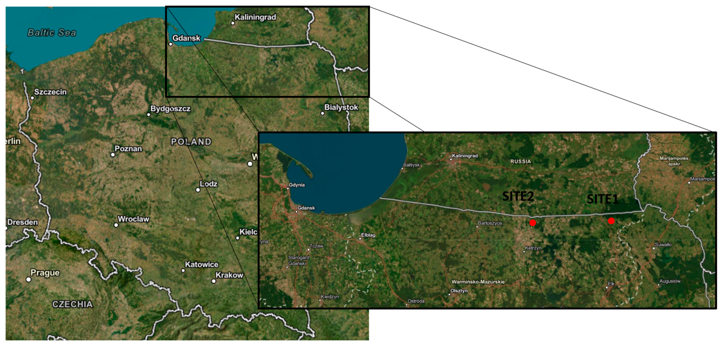
For location SITE1, outlier observations have been removed for the following trees: for tree 1 (height 18 m), the measurement at 0 m has been removed; for tree 5 (height 32 m), measurements at 28 m and 30 m have been removed; for tree 6 (height 16 m), the measurement at 8 m has been removed; and for tree 7 (height 28 m), the measurement at 28 m has been removed. For the second location SITE2, outlier observations have been removed for tree 1 (height 30 m) at the 30 m level; for tree 4 (height 26 m), the measurements at 0 m, 20 m, and 26 m have been removed; for tree 8 (height 26 m), the measurement at 24 m has been removed; and for tree 9 (height 26 m), the measurement at 24 m has been removed. The prepared data was used in subsequent stages. The removal of the observations above was performed for a linearised regression model, which in practice makes it easy from the computational side to check if a given observation is an outlier and effectively influential and if it changes the model fit by at least 1% (R-squared).

At this analysis stage, the two following nonlinear regression functions were obtained: the first, MM, calculated at the ITL level and with the values of the regression function parameters averaged, and the second, M1, calculated at the ATL level. Each approach depends on the goal the researcher has set for themself. Suppose the researcher is interested in individual trees and estimates of different tree parameters. In that case, they will choose the MM, but if the researcher is interested in a large forest area and overall estimates of the whole stand then they will select the M1 model.

In the third stage, the classic model of the nonlinear regression function was initially fitted to each tree separately (ITL). Based on the regression coefficients for individual trees, an overall regression model for all trees was calculated (

Table A2. Fixed effects in the MM for individual trees.

Fixed Effects in the MM	SITE1			SITE2
	${\mathit{\beta }}_{\mathbf{1}}$	${\mathit{\beta }}_{\mathbf{2}}$	${\mathit{\beta }}_{\mathbf{3}}$	${\mathit{\beta }}_{\mathbf{1}}$	${\mathit{\beta }}_{\mathbf{2}}$	${\mathit{\beta }}_{\mathbf{3}}$
tree 1	146	25.99	553	146.5	7.69	1364.9
tree 2	153.8	23.05	559.3	80.52	−1.02	1091.9
tree 3	84.01	21	162.2	177	15.02	1028.2
tree 4	109.8	21	339	83.92	11.31	553
tree 5	146.2	21	611.2	72.26	4.28	553
tree 6	126.5	34.66	553	83.92	11.31	553
tree 7	83.96	4.74	553	138.6	21	519.7
tree 8	57.17	−2.77	553	121.8	26.98	496.6
tree 9	131.7	46.12	394.9	149.6	−23.16	1966.2

), resulting in the marginal model MM (also known as the population-averaged model). The MM was then compared to the nonlinear regression function determined from the values for all trees combined (model M1). Both functions for both locations are shown in Figure 2, and the estimated regression coefficients are given in

Table A4. Random effects in the model M3 for individual trees.

Random Effects in the Model M3	SITE1	SITE2
	${\mathit{b}}_{\mathbf{3}}$	${\mathit{b}}_{\mathbf{1}}$	${\mathit{b}}_{\mathbf{3}}$
tree 1	−24.83	−0.84	0.08
tree 2	−110.62	−1.89	0.16
tree 3	−18.67	0.79	−0.1
tree 4	−48.82	−0.44	0.05
tree 5	−76.56	−0.13	0.02
tree 6	120.13	1.3	−0.18
tree 7	−45.48	0.63	−0.07
tree 8	71.78	−0.02	0.002
tree 9	99.31	0.7	−0.08

.

To compare the fitting of nonlinear regression models, the error ratio to the mean forecast size was expressed in percentage terms as RMSE% (Equation (5)). For SITE1, the fit of the MM was 18.52%, while for the M1 model it was 14.84%. Meanwhile, for SITE2 these values were 24.8% and 24.2%, respectively. The fit of the MM is poorer than that of M1, particularly for SITE1 (Figure 2).

Because the research aimed to find a model that best fits all the trees collectively and each tree individually, the fit of the MM and M1 functions was compared for individual trees (

Table 3. The RMSE% values [%] show the fit of the four analysed regression models to each tree individually in both locations.

SITE1						SITE2
Tree No.	MM	M1	M2	M3	Avg.M3	Tree No.	MM	M1	M2	M3	Avg.M3
1	7.59	8.62	8.33	7.71	9.29	1	10.18	13.76	14.11	10.39	12.98
2	6.91	13.89	9.91	7.18	9.68	2	18.42	32.18	32.32	19.86	21.96
3	7.28	16.76	15.93	13.99	19.2	3	23.54	30.36	30.09	24.14	23.89
4	12.66	14.87	13.87	13.38	16.24	4	6.46	10.08	9.74	7.18	7.03
5	7.53	8.95	7.62	7.73	8.32	5	10.76	10.91	10.75	10.79	11.26
6	12.76	23.45	27.34	14.97	15.11	6	31.15	25.00	26.31	13.26	12.5
7	9.18	12.13	11.80	12.64	10.11	7	21.20	27.50	27.31	23.29	22.29
8	17.43	20.63	22.75	20.83	19.54	8	7.88	10.46	10.74	10.93	9.41
9	8.75	18.74	22.91	13.39	14.69	9	13.56	26.18	25.77	20.77	23.26
Average	10.01	15.34	16.61	12.42	13.58	Average	15.91	20.71	20.79	15.62	16.06

).

The fit of MM to individual trees compared to model M1 was better (the exception being tree 6 in SITE2). However, the fit of MM for all trees combined was worse than that of model M1.

Subsequently, an M2 regression model was specified to account for the possible correlation of residuals within a single tree. The MM and M1 models do not consider the correlation between measurements, i.e., by taking measurements at, e.g., 1.3 m and 2 m or higher, we do not think each second measurement depends on the previous one.

The overall fit of the regression function according to model M2 for all trees was for SITE1, 14.88%, and SITE2, 24.12%, which is comparable to model M1 for both locations. However, the fit of model M2 for individual trees (Table 3) was most often between the fitting results for models MM and M1.

We have three regression functions at this research stage: MM, M1, and M2. We know that the MM function best fits at the ITL level and M1 at the ATL level. However, neither has a good fit at the ITL and ATL levels. Considering the correlations between measurements at successive heights, we found a function M2, whose values at the ITL level are better than M1 but worse than MM, and whose values at the ATL level are close to M1. Considering both ITL and ATL levels, the M2 function is the most universal.

The fourth and most complicated and complex regression function is the M3 model, which considers random effects specific to the given tree in addition to the correlation of residuals (as in the M2 model). In practice, the regression function for the M3 model will have fixed and random coefficients. It should combine the advantages of the MM and M1 functions and consider the correlations between the results of the M2 function. The random components in the regression model should consider the tree’s nature. By taking measurements, the researcher does not see differences between trees of the same age growing in a similar forest environment. One may only notice that one tree is slightly thinner or thicker. It is only possible to talk about BT when all the measurements are taken together. To account for these slight differences in tree characteristics, we introduce random effects into the regression model, which should show us the individual characteristics of each tree in a single universal regression function.

The first problem with such a complex function is determining good starting values, as the methods for determining the parameters of the nonlinear regression function are iterative. When determining the model’s parameters, known boundary values or asymptotes of the regression function can be used [24,25,28]. In practice, we most often do not see the boundary values of the dependent variable (the asymptote of the model). Due to the model’s complex form, we cannot provide starting values. In such a situation, fitting models with different random effects, b_i (Equation (3)), remains. Although this is a monotonous method, with computers and good statistical software at one’s disposal it is possible to check all combinations of random effects and select the best-fitting model based on, for example, the Schwarz BIC. Schwarz’s BIC was used to compare the fit quality of regression functions with different random effects (

Table 4. Fitting regression models with a different number of random components, b_i, based on BIC values (models with lower BICs are preferred) and the convergence of the iterative method.

Random Components			BIC SITE1	The Convergence	BIC SITE2	The Convergence
b1	b2	b3	123.7	yes	228.8	yes
b1	b2		123.7	yes	228.8	yes
b1		b3	139.4	non-convergence	223.2	yes
	b2	b3	125.2	yes	230.2	yes
		b3	123.5	yes	225.9	yes
	b2		127.5	non-convergence	232.4	non-convergence
b1			123.6	non-convergence	225.4	non-convergence

). Schwarz proposed a Bayesian information criterion (BIC) that provides a criterion for model selection: models with lower BICs are preferred. The Bayesian information criterion (BIC) measures model performance by considering model complexity. The large availability of procedures for calculating BIC values provides a quick and easy way to compare models.

To fit the M3 model, the following were considered: 1. various combinations of the three random components b_i (Equation (3)); 2. convergence of the iterative method; 3. the value of the BIC (Table 4). For the location SITE1 the best combination of random components was the combination with only b₃ (Equation (6)), while for SITE2 it was the combination of the two components b₁ and b₃ (Equation (7)). These are represented as follows:

$$BT={\displaystyle \frac{{\beta }_1}{{\beta }_2+\frac{{\beta }_3+b_3}{SD}}},\text{ M3 regression function for SITE1}$$

(6)

$$BT={\displaystyle \frac{{\beta }_1+b_1}{{\beta }_2+\frac{{\beta }_3+b3}{SD}}},\text{ M3 regression function for SITE2}$$

(7)

where ${\beta }_i$ when I = 1,2,3 are fixed effects and b_j when j = 1, 3 are random effects. The estimated fixed and random regression effects are given in

Table A3. Fixed effects in the models MM, M1, M2, and M3 for all trees in each site.

Fixed Effects	SITE1				SITE2
	MM	M1	M2	M3	MM	M1	M2	M3
${\beta }_1$	115.46	113.4	23.12	118.79	117.12	143.2	22.91	7.85
${\beta }_2$	21.64	14.95	3.3	19.02	8.16	12.58	1.82	0.56
${\beta }_3$	475.4	553	98.7	520.7	902.94	983.4	162.64	56.73

and Table A4.

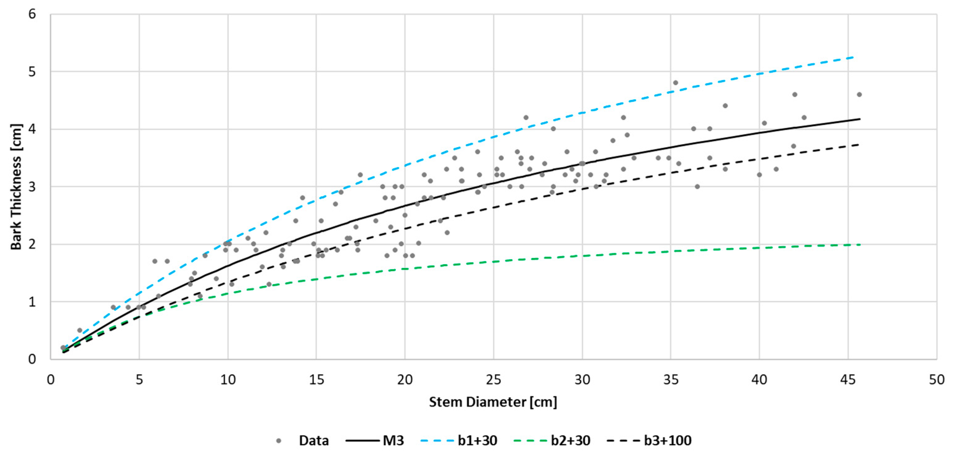
One can also use graphs when selecting random effect components for the M3 model. It is necessary to compare the trajectory of the averaged regression function M3 with the simulation graphs (Figure 3). The simulation graphs show how the trajectory of the averaged M3 model changes depending on variations in the values of the random effect coefficients b₁, b₂, and b₃. In our case, a shift in b₁ increases the estimates of BT at high D values, while a change in b₂ decreases the BT estimates at high D values. Meanwhile, a change in b₃ causes a parallel shift in the graph across nearly the entire trajectory of the regression function.

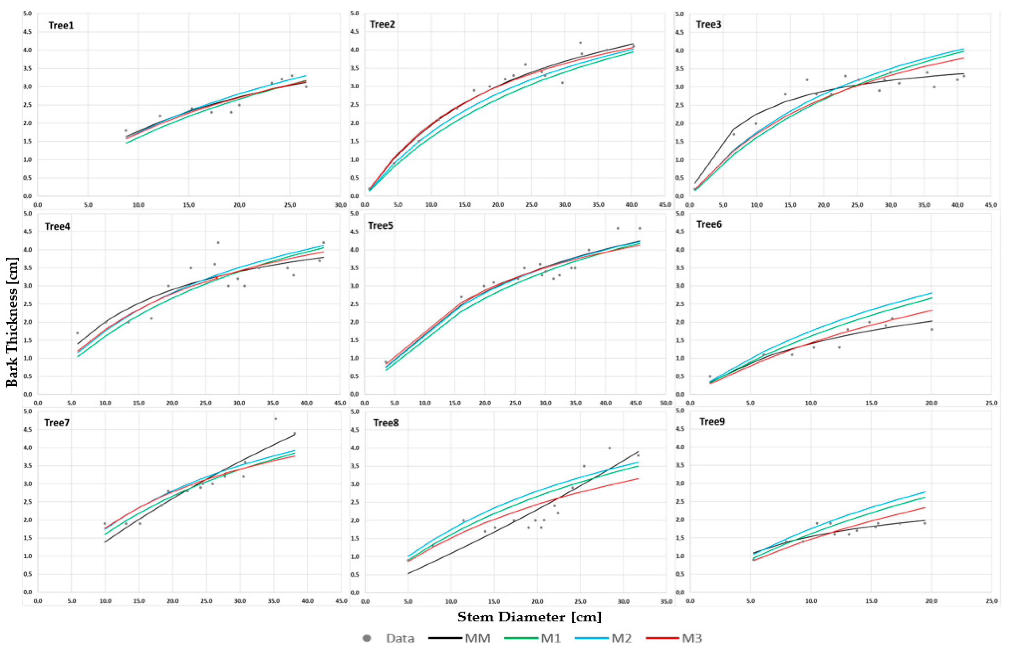
To determine which random effects are significant for individual trees (ITL), it is necessary to compare the shift in the estimated function M3 against the position of the regression function without random effects, namely model M2 (Figure 4 and Figure 5, model M3—red, M2—blue). In SITE1 (Figure 4) for trees 1, 3, 6, 8, and 9, the position of function M2 is above that of function M3, indicating an overestimation of BT values. Conversely, for tree 2 the position of M2 is below that of model M3, indicating an underestimation of BT. In SITE2 (Figure 5) the position of function M2 for trees 1, 2, and 4 is above that of function M3, whilst for trees 3, 6, 7, and 9 it is below the function for model M3. The shift in the graph close to parallel corresponds to the random effect b₃. However, it is harder to notice the influence of the impact of b₁ on the graphs, which is observable if the parallel shift in graph M2 compared to M3 is disturbed upwards or downwards. The graphs for trees 2, 3, 4, 6, 7, and 9 in SITE2 exhibit such a disturbance, which is confirmed by the low BIC value for model M3 with random effect b₁. In SITE1 such a disturbance can only be observed for two trees (3 and 6), which confirms that the selection of model M3, with only the random component b₃ obtained through BIC, was appropriate.

The fit of model M3 to all trees (ATL) for the location SITE1 was 12.49%, and for SITE2 it was 19.05%. Compared to previous models, these were the best fits. However, the fit of model M3 for individual trees (ITL), compared to MM, was slightly worse, but in most cases it was better than models M1 and M2 (Table 3). Considering the differences between the average RMSE% (Table 3) in the individual fit to trees at location SITE1, it is evident that model M1 had a worse fit than MM by an average of 5.33%, model M2 by 5.6%, and model M3 by 2.41%. Meanwhile, at SITE2, compared to MM, worse fits were obtained for M1 by 4.8%, M2 by 4.88%, and for M3 a better fit was obtained by 0.29%. At location SITE2 the exception was tree 6, for which the fits, compared to MM, were better: M1 by 6.15%, M2 by 4.84%, and M3 by 17.98%.

In Figure 4 and Figure 5 the fit for individual trees can be traced. For models M1 and M2 about MM there is often an overestimation, meaning that the graphs for M1 and M2 lie above MM (for SITE1: tree 6 and tree 9, for SITE2: tree 1, tree 2, tree 4, and tree 6) or an underestimation, meaning that the graphs for M1 and M2 lie below MM (for SITE1: tree 2 and tree 5, for SITE2: tree 3 and tree 7). For the remaining trees the regression function graphs for M1 and M2 intersect with MM. However, the regression function graph for M3 runs between MM and M1 or M2 and is always close to the points representing the data.

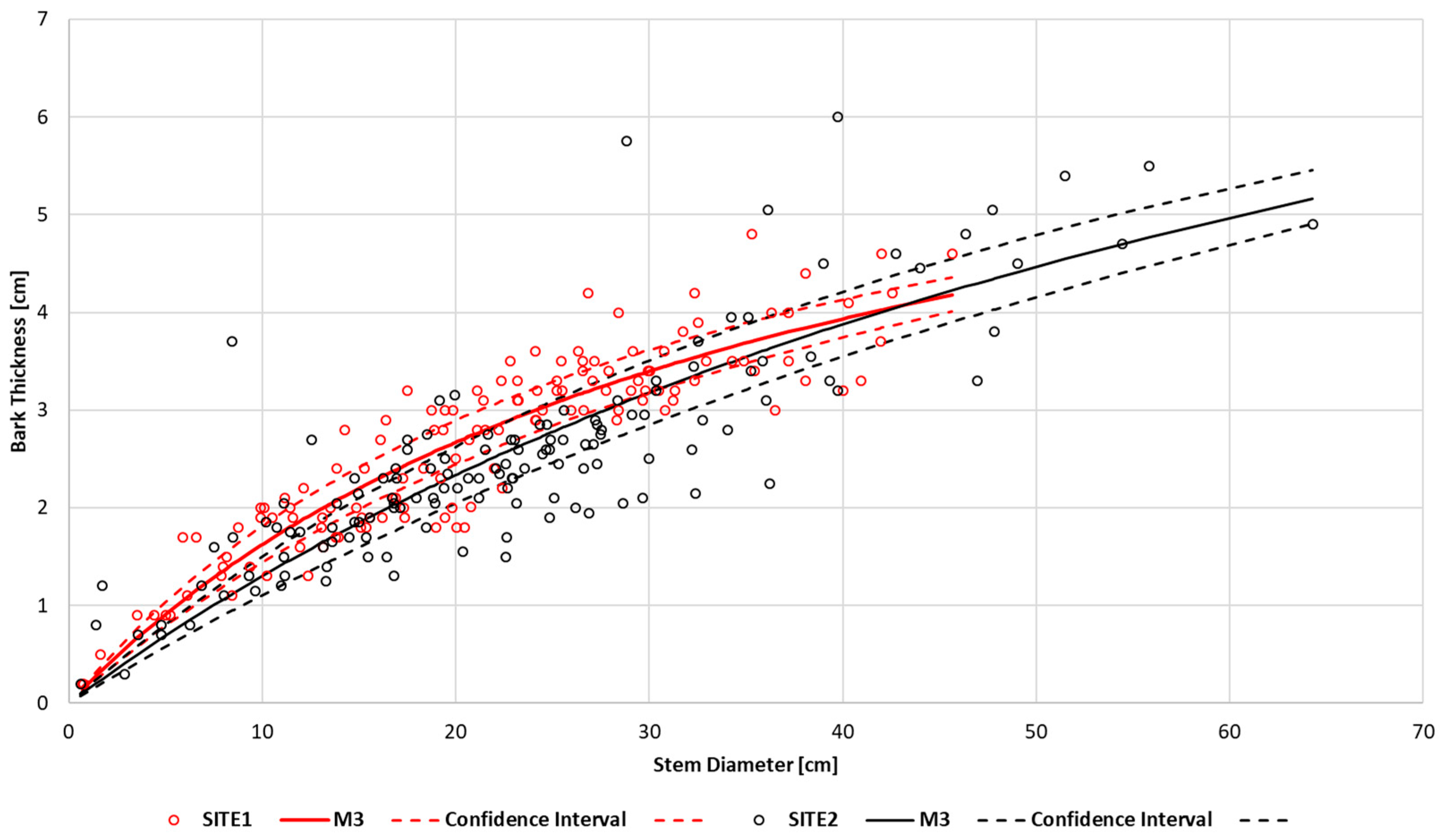
To demonstrate the regression functions of M3 for each location, it is necessary to average them as the values of the random effects differ for each tree. Figure 6 presents the regression functions of M3 along with confidence intervals for locations SITE1 and SITE2. By comparing the course of the confidence interval graphs, it can be concluded that there are no significant differences between the average bark thicknesses at both locations. For this reason, we calculated the averaged regression function for both locations (Figure 6, Table 3). The overall fit of the resulting regression function is at a level of 19.67% (ATL). Regarding the analysis for individual trees, considering the differences between the average RMSE%, the average regression function’s fit compared to the MM for SITE1 was worse by 3.56% and for SITE2 by 2.51% (Table 3). However, the individual fit of this function is worse than that of the M3 model but better than the fit of models M1 and M2.

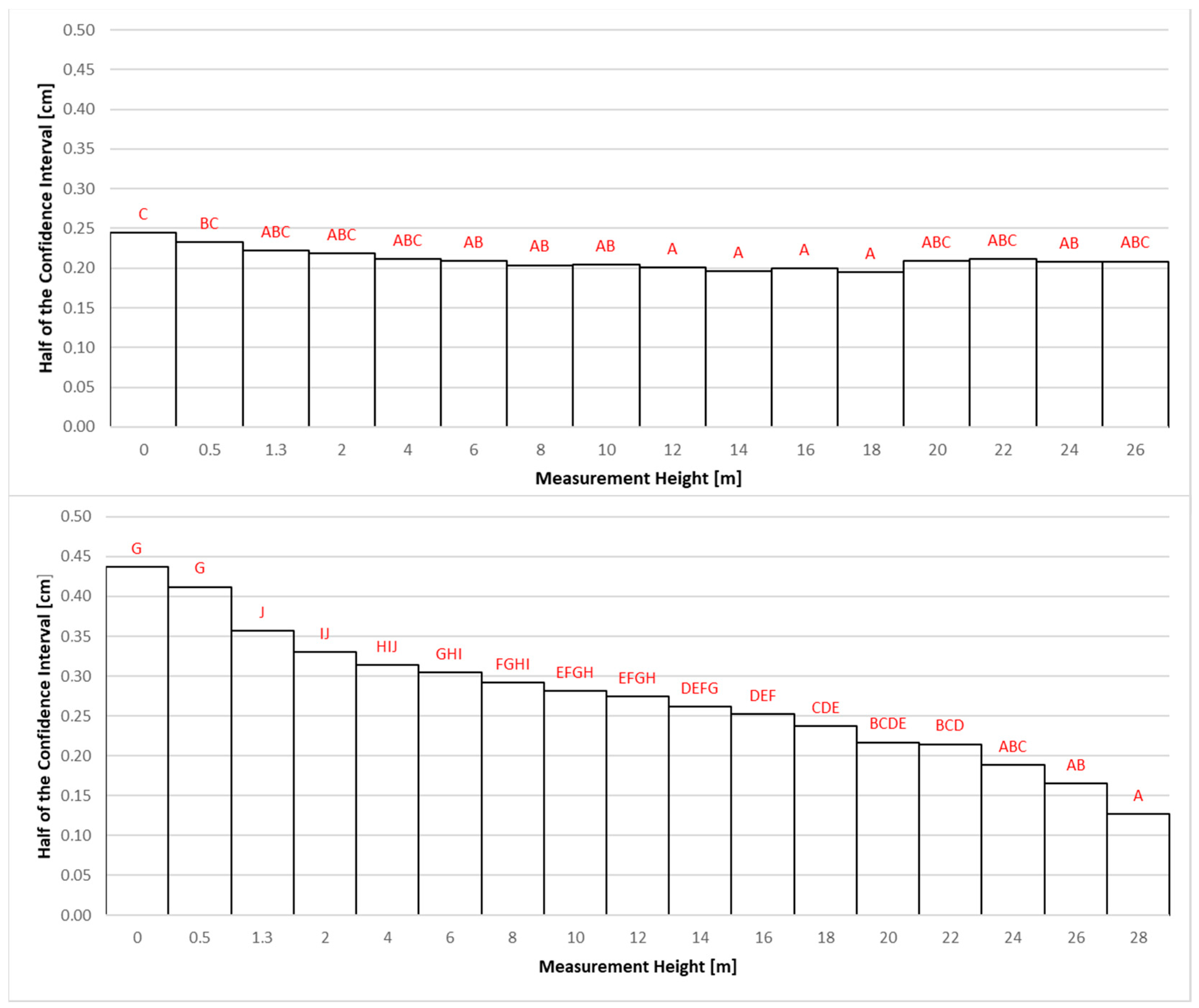
The final stage of the research was to check the accuracy of estimating the average thickness of bark at different measurement heights. For this purpose, at each height where the bark thickness was measured (0, 0.5, 1.3, 2 m, and then every 2 m up to the top), confidence interval halves were determined for the M3 regression function for both locations. Treating each tree as a replicate, a one-way analysis of variance was conducted. Homogeneous groups were established using Tukey’s test (Figure 7).

In location SITE1, the largest deviations (the greatest prediction error of the average) from the estimated mean bark thickness were recorded at the base of the tree (0 m) and a height of 0.5 m (Figure 7). The smallest deviations (the least prediction error of the average) were obtained at heights between 12 and 18 m. For location SITE2, a decrease in deviations from the estimated mean bark thickness (continuous improvement in average predictions) with an increase in measurement height can be observed. The largest deviations occurred at the tree’s base and heights of 0.5 m and 1.3 m, while the smallest were at 26 and 28 m heights. The observed differences in the precision of BT estimation between analysed sites may result from the difference in the age of the investigated trees (50 vs. 63 years). However, a clear pattern in which the lowest parts of the tree exhibit the highest inaccuracy is shared between the studied plots.

4. Discussion

In research on the variability of bark thickness (BT), the most commonly used explanatory variable is stem diameter (D), typically measured at a height of 1.3 m (DBH). Rosell [33], using a linear regression function, demonstrated that stem diameter can explain 72% (calculated using R-squared) of the overall variability in BT. In our studies, due to the comparison of simple nonlinear models and nonlinearizable models (MM and M1) with complex nonlinear models (M2, M3), we could not apply the R-squared coefficient of determination. Instead, we used the RMSE% measure for model comparison. However, for model M3 we calculated the adjusted R-squared to compare our results with those obtained in other studies. The fit of our proposed regression function M3 for SITE1 was 87.44%, and for SITE2 it was 80.6%, indicating a significantly better explanation of BT variability by D compared to earlier works. Another advantage of the M3 regression model is that it estimates BT at any measurement height, not just at a height of 1.3 m (DBH).

Considering the complexity of the bark thickness models, modelling has two directions. In the first, simple linear regression models are used. In a study [1], an analysis of bark thickness was conducted depending on stem diameter and the distance from the base of the stem. Simple models, referred to in our work as MM and M1, were utilised, and they are easy to apply in practice. At this study stage, we must know we will not obtain a universal regression function at ITL and ATL levels. Choosing the MM will result in significant errors in feature estimates for whole stands, and choosing M1 will not be a good choice for characterisation and comparisons at the ITL level.

Forecasting uses measurements at a single height to eliminate issues with repeated data (M2), i.e., DBH [2,5,6]. This direction includes studies on tree mortality assessment (depending on BT) caused by fire [4]. The applied simple logistic regression models were substitutes for more complex nonlinear models, M1, and did not require estimating starting values for iterative calculations. In modelling bark thickness, with the help of simple models MM or M1, an attempt was made to achieve more than 70% variability in BT as explained by R-squared. The downside of this approach was modelling BT based on a single D measurement at 1.3 m (DBH). Our proposed M3 regression model allows BT to be predicted from a D measurement at any tree height. The percentage of explained variation based on the M3 model can be more than 80% (the adjusted R-squared).

Models with more variables were selected, or artificial/transformed variables were introduced to explain as much variability as possible. In another study [34], the thickness of the bark of Pinus radiata D. Don was predicted based on the diameter above the bark, position up the stem, tree height, and diameter above the bark at breast height, as well as an artificial variable of the type (h/H)—level of measurement above ground [m]/total tree height [m]. Similarly, in another study [35], the thickness of the bark at any point along the stem of Eucalyptus pilularis, E. obliqua, E. andrewsii, E. saligna, and Corymbia maculata was estimated depending on the diameter above the bark at that point, the height above the ground at the measurement point along the stem, total tree height, and breast height above the bark. Similarly, some studies [36,37] present several variables related to differences in the structure of the bark and the proportions of the inner and outer bark. The strength of the MM function was its good individual fit for trees (ITL) and the use of only one D variable. Using a single explanatory variable makes it very easy to describe the characteristics of the tree, and good model fitting guarantees minor errors. The determined models MM, M1, M2, and M3 share the common feature of having only one explanatory variable.

Since our four presented models differ in calculating and considering correlations between measurements and random changes between trees, we show the advantages and disadvantages. The MM became a benchmark when comparing results for the more complex models M2 and M3 concerning individual fitting for each tree. In contrast, the advantage of the M1 model was its good overall fitting to all trees (ATL). As a result, the M1 model became the benchmark for the more complex models M2 and M3 regarding overall fitting to all trees. In contrast, the M3 model proved to be the most universal.

In the second direction of the research, complex regression models are used. The study in [10] examined spatial dependencies or spatial autocorrelations. Relatively simple functions from the M2 model group were applied. Among the complex models, nonlinear regression functions with mixed effects were used [11,14]. However, these models did not consider the influence of correlations resulting from repeated measurements, meaning they were simple models serving as the basis for deriving the formula for the M3 model. A similar situation occurred in the studies [38], where nonlinear regression functions used in harvesters to estimate the diameter under the bark were examined and modified based on bark measurements. The modifications to these functions [39] were so complicated that SAS system 8.02 procedures [40] NLIN, MIXED, and REG were used for the calculations. Considering the SAS system 8.02 procedures set, models such as M2 and M3 were complicated. A good example of the application of the complex M3 model is found in the study in [16], which demonstrates how straightforward the results obtained from the complex M3 regression functions can be in practice. The application we present in this paper may suggest another direction of M3-like model usage, i.e., determination of the various parameters along the stem, which might be performed, e.g., by harvesters.

This research follows a similar trajectory to historical growth curve modelling studies (e.g., orange trees), where models evolved from simple functions to complex mixed-effects approaches [18]. The results were re-evaluated in works [41,42], where a more complex logistic model of the growth curve was proposed. The last proposal for analysing this data was a model with repeated measures and random effects calculated using the NLINMIXED procedure in the SAS system in the study from [21]. The NLINMIXED procedure was initially written to implement the algorithm of Lindstrom and Bates [43]. Our research may reflect the described historical process of improving the regression model of the growth curve of orange trees.

We started with simple nonlinear MM and M1 models, whose advantages were a good fit at the ITL level for the MM and a good fit at the ATL level for the M1 model. Unfortunately, none of these models were nulliparous, meaning they fit well at both levels.

The second step was to use repeated measurements in the M2 model, i.e., we considered the correlations between measurements at different tree heights. The results obtained for model M2 indicated that considering the correlation between observations was a valid assumption. The M2 model at the ITL level was worse than the MM but better than the M1, and at the ATL level it was comparable to the M1 model.

In the third step of the model M2 we added random effects, resulting in the model M3. Model M3 accounted for random variations between the trees. For model M3 (ITL) at SITE1 the RMSE% coefficient obtained was on average 2.41% worse than MM, while at SITE2 it was 0.29% better (Table 3). For all trees (ATL) the RMSE% for model M3 was 12.49% at SITE1 and 19.05% at SITE2, and it was better than the RMSE% of model M2 (SITE1 14.84% and SITE2 24.2%). Considering the above results, it can be said that the regression functions determined for model M3 (Equations (6) and (7)) meet both conditions set out for the work as they are well fitted both individually and overall for all trees, indicating that the objective of the work has been achieved.

In the final stage of the research, the regression functions designated according to the M3 model were used to check how the estimation error of bark thickness (the midpoint of the 95% confidence interval for the regression function) varies at different measurement heights (Figure 7). The obtained results may indicate at which heights to measure the diameter to achieve the most accurate estimates of bark thickness. Due to our observation of a decrease in deviations from the forecasted average bark thickness with an increase in height, it is worthwhile to consider additional measurements at greater heights than DBH in practice. An elaborate model construction methodology may be used for programming algorithms in harvesters so that the under-bark volume of a stem or log could be calculated directly during its manipulation by the machine. It might also provide valuable solutions, e.g., biomass estimation modelling, so that the biomass of the bark component can be more easily calculated. However, those prospective applications require further studies on accuracy and workload.

References

1. Konôpka, B.; Pajtík, J.; Šebeň, V.; Merganičová, K. Modeling Bark Thickness and Bark Biomass on Stems of Four Broadleaved Tree Species. Plants 2022, 11, 1148. [Google Scholar] [CrossRef]
2. Biging, G.S. Taper equations for second-growth mixed conifers of Northern California. For. Sci. 1984, 30, 1103–1117. [Google Scholar]
3. Amidon, E.L. A general taper functional form to predict bole volume for five mixed-conifer species in California. For. Sci. 1984, 30, 166–171. [Google Scholar]
4. Ryan, K.C.; Reinhardt, E.D. Predicting postfire mortality of seven western conifers. Can. J. For. Res. 1988, 18, 1291–1297. [Google Scholar] [CrossRef]
5. Hengst, G.E.; Dawson, J.O. Bark properties and fire resistance of selected tree species from the central hardwood region of North America. Can. J. For. Res. 1994, 24, 688–696. [Google Scholar] [CrossRef]
6. Bronisz, K. Modeling of the tree and stand parameters using mixed-effects models. Sylwan 2019, 163, 564–575. [Google Scholar]
7. Bronisz, K.; Gruchała, A.; Zasada, M. Modelling the bark thickness along the trunk with taper models. Sylwan 2019, 163, 469–478. [Google Scholar]
8. Landsberg, J.J. Physiological Ecology of Forest Production; Academic Press: New York, NY, USA, 1986; p. 198. [Google Scholar]
9. Burkhart, H.E.; Gregoire, T.G. Forest biometrics. In Handbook of Statistics. v. 12: Environmental Statistics; Patil, G.P., Rao, C.R., Eds.; Elsevier Science: Amsterdam, The Netherlands, 1994; pp. 377–407. [Google Scholar]
10. Fox, J.C.; Ades, P.K.; Bi, H. Stochastic structure and individual-tree growth models. For. Ecol. Manag. 2001, 154, 261–276. [Google Scholar] [CrossRef]
11. Hall, D.B.; Clutter, M. Multivariate Multilevel Nonlinear Mixed Effects Models for Timber Yield Predictions. Biometrics 2004, 60, 16–24. [Google Scholar] [CrossRef]
12. Bauer, R.; Billard, A.; Mothe, F.; Longuetaud, F.; Houballah, M.; Bouvet, A.; Cuny, H.; Colin, A.; Colin, F. Modelling bark volume for six commercially important tree species in France: Assessment of models and application at regional scale. Ann. For. Sci. 2021, 78, 104. [Google Scholar] [CrossRef]
13. Jenkins, J.C.; Chojnacky, D.C.; Heath, L.S.; Bsey, R.A. National scale biomass estimators for United States tree species. For. Sci. 2003, 49, 12–35. [Google Scholar] [CrossRef]
14. Stängle, S.M.; Sauter, U.H.; Dormann, C.F. Comparison of models for estimating bark thickness of Picea abies in southwest Germany: The role of tree, stand, and environmental factors. Ann. For. Sci. 2017, 74, 16. [Google Scholar] [CrossRef]
15. Stängle, S.M.; Dormann, C.F. Modelling the variation of bark thickness within and between European silver fir (Abies alba Mill.) trees in Southwest Germany. Forestry 2018, 91, 283–294. [Google Scholar] [CrossRef]
16. Tyburski, L.; Przybylski, P.; Ukalski, K.; Konatowska, M.; Rutkowski, P. Long-term analysis of sap flow conditions in the trunk of Scots pine (Pinus sylvestris L.) in the old-growth phase in relation to air temperature. Folia For. Pol. Ser. A-For. 2024, 66, 215–227. [Google Scholar]
17. Daniel, C.; Wood, F. Fitting Equations to Data, Revised ed.; John Wiley & Sons: New York, NY, USA, 1980. [Google Scholar]
18. Draper, N.R.; Smith, H. Applied Regression Analysis, 2nd ed.; John Wiley & Sons: New York, NY, USA, 1981. [Google Scholar]
19. Weisberg, S. Applied Linear Regression; John Wiley & Sons: New York, NY, USA, 1980. [Google Scholar]
20. Verbeke, G.; Molenberghs, G. Linear Mixed Models for Longitudinal Data; Springer: New York, NY, USA, 1997. [Google Scholar]
21. Vonesh, E.F. Generalized Linear and Nonlinear Models for Correlated Data: Theory and Applications Using SAS; SAS Institute Inc.: Cary, NC, USA, 2012. [Google Scholar]
22. SAS Institute Inc. SAS/STAT 14.3 User’s Guide; SAS Institute Inc.: Cary, NC, USA, 2017. [Google Scholar]
23. Pinheiro, J.C.; Bates, D.M. Approximations to the Log-Likelihood Function in the Nonlinear Mixed-Effects Model. J. Comput. Graph. Stat. 1995, 4, 12–35. [Google Scholar] [CrossRef]
24. Bates, D.M.; Watts, D.G. Nonlinear Regression Analysis and Its Applications; John Wiley & Sons: New York, NY, USA, 1988. [Google Scholar]
25. Ratkowsky, D.A. Nonlinear Regression Modeling: A Unified Practical Approach; Marcel Dekker, Inc.: New York, NY USA, 1983. [Google Scholar]
26. Schwarz, G.E. Estimating the dimension of a model. Ann. Stat. 1978, 6, 461–464. [Google Scholar] [CrossRef]
27. Davidian, M.; Giltinan, D.M. Nonlinear Models for Repeated Measurement Data; Chapman & Hall: New York, NY, USA, 1995. [Google Scholar]
28. Vonesh, E.F.; Chinchilli, V.M. Linear and Nonlinear Models for the Analysis of Repeated Measurements; Marcel Dekker: New York, NY, USA, 1997. [Google Scholar]
29. Spiess, A.N.; Neumeyer, N. An evaluation of R2 as an inadequate measure for nonlinear models in pharmacological and biochemical research: A Monte Carlo approach. BMC Pharmacol. 2010, 10, 6. [Google Scholar] [CrossRef] [PubMed]
30. Mayer, D.; Butler, D. Statistical validation. Ecol. Modell. 1993, 68, 21–32. [Google Scholar] [CrossRef]
31. Vonesh, E.F.; Chinchilli, V.M.; Pu, K. Goodness-of-Fit in Generalized Nonlinear Mixed-Effects Models. Biometrics 1996, 52, 572–587. [Google Scholar] [CrossRef]
32. Motulsky, H.J.; Brown, R.B. Detecting outliers when fitting data with nonlinear regression—A new method based on robust nonlinear regression and the false discovery rate. BMC Bioinform. 2006, 7, 123. [Google Scholar] [CrossRef]
33. Rosell, J.A. Bark thickness across the angiosperms: More than just fire. New Phytol. 2016, 211, 90–102. [Google Scholar] [CrossRef] [PubMed]
34. Gordon, A. Estimating bark thickness of Pinus radiata. N. Z. J. For. Sci. 1983, 13, 340–348. [Google Scholar]
35. Charles, K.M. Bark thickness equations for five commercial tree species in regrowth forests of Northern New South Wales. Aust. For. 2000, 63, 34–43. [Google Scholar]
36. Paine, C.E.T.; Stahl, C.; Courtois, E.A.; Patiño, S.; Sarmiento, C.; Baraloto, C. Functional explanations for variation in bark thickness in tropical rain forest trees. Funct. Ecol. 2010, 24, 1202–1210. [Google Scholar] [CrossRef]
37. Hempson, G.P.; Midgley, J.J.; Lawes, M.J.; Vickers, K.J.; Kruger, L.M. Comparing bark thickness: Testing methods with bark–stem data from two South African fire-prone biomes. J. Veg. Sci. 2014, 25, 1247–1256. [Google Scholar] [CrossRef]
38. Hannrup, B. Funktioner för skattning av barkens tjocklek hos tallvoch gran vid avverkning med skördare; Skogforsk: Uppsala, Sweden, 2004. [Google Scholar]
39. Zacco, P. Barktjockleken hos sågtimmer; Rapport nr. 90; Institutionen för Virkeslära, Skogshögskolan: Stockholm, Sweden, 1974; pp. 1–53. [Google Scholar]
40. SAS Institute Inc. SAS/STAT User’s Guide, version 8; SAS Institute Inc.: Cary, NC, USA, 1999; ISBN 1-58025-494-2. [Google Scholar]
41. Lindstrom, M.J.; Bates, D.M. Nonlinear mixed effects models for repeated measures data. Biometrics 1990, 46, 673–687. [Google Scholar] [CrossRef]
42. Pinheiro, J.C.; Bates, D.M. Mixed-Effects Models in S and S-PLUS; Springer: New York, NY, USA, 2000. [Google Scholar]
43. Wolfinger, R. Comment: Experience with the SAS macro NLINMIX. Stat. Med. 1997, 16, 1258–1259. [Google Scholar]
Figure 1. Location of Site1 and Site2 (background source: https://www.bdl.lasy.gov.pl/portal/mapy-en, URL accessed on 28 May 2025).
Forests 16 01160 g001
Figure 2. Graphs of nonlinear regression functions for the marginal model (MM) and model M1 (location SITE1 on the (left), SITE2 on the (right)).
Forests 16 01160 g002
Figure 3. Simulated graphs of regression functions M3 depending on the random effect b1, b2, or b3. The results are derived from the location SITE1.
Forests 16 01160 g003
Figure 4. Regression functions for models MM, M1, M2, and M3 for individual trees (ITL) at location SITE1. Bark thickness [cm]—vertical axis; stem diameter [cm]—horizontal axis; data—grey dots; MM—black line; M1—green line; M2—blue line; M3—red line. Higher resolution figures are in Figure S1.
Forests 16 01160 g004
Figure 5. Regression functions for models MM, M1, M2, and M3 for individual trees (ITL) at location SITE2. Bark thickness [cm]—vertical axis; stem diameter [cm]—horizontal axis; data—grey dots; MM—black line; M1—green line; M2—blue line; M3—red line. Higher resolution figures are in Figure S2.
Forests 16 01160 g005
Figure 6. Averaged regression function charts for locations SITE1 and SITE2, with confidence intervals. Bark thickness [cm]—vertical axis; stem diameter [cm]—horizontal axis.
Forests 16 01160 g006
Figure 7. Homogeneous groups for half the confidence interval of the regression function M3 at different measurement heights. The upper chart presents results for SITE1 and the lower one for SITE2.
Forests 16 01160 g007