Predicting Forest Trail Degradation Susceptibility Using GIS-Based Explainable Machine Learning

Abstract

Effective trail management is essential for preventing environmental degradation and promoting sustainable recreational use. This study proposes a GIS-based, explainable machine learning framework for predicting forest trail degradation using exclusively environmental variables, eliminating the need for costly visitor monitoring data that remains unavailable in most operational forest settings. Field surveys conducted in Geumjeongsan, South Korea, classified trail segments as degraded or non-degraded based on physical indicators such as erosion depth, trail width, and soil hardness. Environmental predictors—including elevation, slope, trail slope alignment (TSA), topographic wetness index (TWI), vegetation type, and soil texture—were derived from spatial analysis. Three machine learning algorithms (Binary Logistic Regression, Random Forest, and Gradient Boosting) were systematically compared using confusion matrix metrics and AUC-ROC (Area Under the Receiver Operating Characteristic Curve). Random Forest (RF) was selected for its strong performance (AUC-ROC = 0.812) and seamless integration with SHAP (SHapley Additive exPlanations) for transparent interpretation. Spatial block cross-validation achieved an AUC-ROC of 0.729, confirming robust spatial generalization. SHAP analysis revealed vegetation type as the most significant predictor, with hardwood forests showing higher degradation susceptibility than mixed forests. A susceptibility map generated from the RF model indicated that 40.7% of the study area faces high to very high degradation risk. This environmental-only approach enables proactive trail management across data-limited forest systems globally, providing actionable insights for sustainable trail maintenance without requiring visitor use data.

1. Introduction

Forest ecosystems provide essential ecological services while serving as increasingly important recreational resources for urban populations [1,2]. Trail-based recreation has become a cornerstone of sustainable forest management, offering opportunities for environmental education, public health benefits, and eco-tourism [3,4,5]. However, intensive recreational use creates substantial management challenges, as trail impacts—including soil erosion, vegetation trampling, and habitat fragmentation—can compromise long-term ecosystem integrity [6,7,8]. Forest managers face the complex task of balancing public access with ecological protection, requiring science-based approaches that can anticipate and prevent irreversible degradation [9,10,11,12].

Successful trail management hinges on understanding the spatial patterns of environmental susceptibility across forest landscapes [13,14]. Trail degradation manifests through interconnected processes including surface erosion, root exposure, soil compaction, and vegetation loss, with impact severity largely determined by topographic, edaphic, and vegetation characteristics [6,15]. While recreational pressure initiates these processes, underlying environmental conditions control which locations develop severe degradation and which remain stable under comparable use intensity [15,16]. Research has demonstrated an asymptotic relationship between trail damage and visitor use, where initial impacts trigger disproportionate degradation that stabilizes over time, suggesting that environmental factors—including slope alignment, substrate types, and vegetation characteristics—may be more influential than use intensity in determining long-term degradation patterns [17,18]. This relationship provides the foundation for predictive approaches that can guide proactive management decisions.

Conventional trail assessment methods rely predominantly on field surveys and professional judgment—approaches that, while valuable, are resource-intensive and difficult to implement systematically across extensive forest networks [13,14]. These methods often fail to capture the multivariate environmental relationships that govern degradation patterns, limiting their predictive capability [19,20]. Furthermore, most research frameworks depend on detailed visitor use data that remains unavailable in the majority of operational forest settings due to monitoring costs and logistical constraints [15,17]. Forest managers require practical alternatives that can utilize existing spatial datasets to identify high-degradation susceptibility areas efficiently.

Advances in geographic information systems and spatial data processing have created new opportunities for predictive forest management [16,18]. Digital elevation models, vegetation mapping, and soil databases—while requiring technical processing—are increasingly accessible through national forestry programs and remote sensing platforms [21,22]. Machine learning techniques have proven effective for analyzing these complex spatial datasets, with successful applications in erosion modeling and habitat assessment [23,24]. Trail-specific studies have demonstrated promising results: Tomczyk and Ewertowski [16] effectively predicted trail width patterns using environmental variables, while Sahani and Ghosh [25] achieved robust degradation susceptibility assessments through ensemble modeling approaches.

However, operational forest management requires analytical approaches that balance predictive accuracy with interpretability and practical feasibility [26]. While recent machine learning advances offer powerful predictive capabilities, their varying characteristics must be carefully considered: Random Forest provides robust predictions with inherent feature importance metrics, Gradient Boosting techniques may achieve marginally higher accuracy but require additional interpretation tools, and Logistic Regression offers statistical transparency but struggles with non-linear environmental interactions [27,28]. Given these trade-offs, the selection of appropriate methods must prioritize both performance and practical utility for forest management contexts.

Furthermore, the need for explainable machine learning approaches has been increasingly emphasized in environmental management, particularly in forestry and conservation, where decision-makers require interpretable insights to guide sustainable practices [26]. In this context, SHAP analysis was applied to enhance the interpretability of the Random Forest model by quantifying the contribution of each environmental variable to prediction outcomes. This approach ensures that model-driven trail degradation assessments remain transparent and actionable, supporting sustainable management strategies.

Therefore, this study develops a spatially explicit framework for predicting trail degradation susceptibility using environmental variables derivable from standard forest management datasets. We employ Random Forest and SHAP analysis as our primary approach while validating their effectiveness against Logistic Regression and Gradient Boosting to confirm that the interpretability benefits do not come at the expense of predictive performance. This framework prioritizes practical utility for forest management, demonstrating that RF and SHAP provide both competitive accuracy and the transparency essential for operational decision-making.

2. Materials and Methods

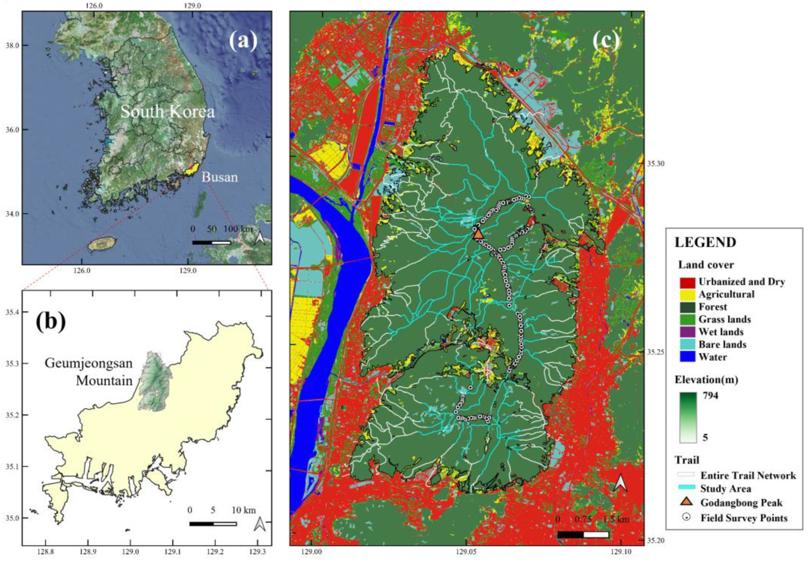
2.1. Study Area

The Korean Peninsula encompasses approximately 10,041,000 hectares, of which 62.7% is forested (Figure 1a). Busan, located in the southeastern region (35.18° N, 129.08° E), contains 45,926 hectares of forested areas (59.7% of the city’s total area) (Figure 1b) [29].

Geumjeongsan, the highest mountain in Busan (801.5 m at Godangbong peak), covers approximately 5170 hectares and serves as both an ecological habitat and major recreational area within the urban landscape (Figure 1b). The mountain features diverse terrain including steep slopes, valleys, and ridgeline systems, with annual precipitation averaging 1597.2 mm [30]. Despite hosting 1782 documented species (including 13 endangered species) [31], Geumjeongsan experiences intense recreational pressure with approximately 3.12 million annual visitors [32]. The mountain is surrounded by urbanized areas according to LULC classifications, facilitating high accessibility (Figure 1c). The extensive trail network developed over centuries and the absence of systematic visitor monitoring make it an ideal site for developing environmental variable-based degradation models.

Trail network data from the Korea Forest Service [29] and land cover data from the Ministry of Environment [33] were utilized for analysis. From 210.16 km of total trail networks, 89.1 km of forested segments was identified, with 14.5 km selected for a field survey. Survey points ranged from 346 to 757.5 m in elevation. Following spatial modeling best practices [34], areas below 346 m were excluded to prevent extrapolation beyond the observed conditions, ensuring model reliability and interpretability.

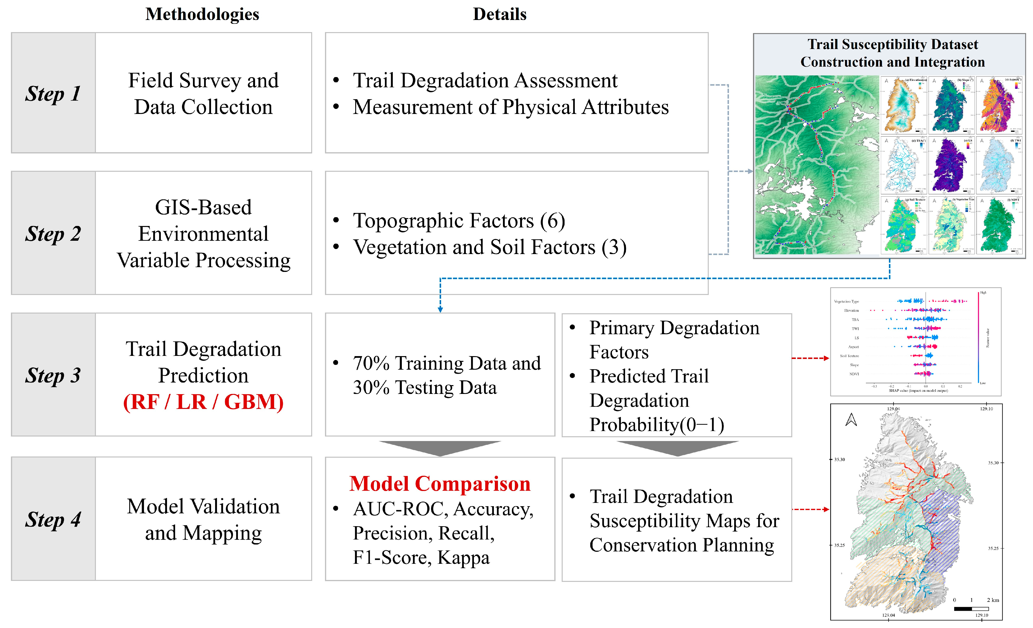
2.2. Research Framework

This study adopted a four-step methodological framework to evaluate and predict trail degradation susceptibility (Figure 2). First, a comprehensive field survey was conducted to classify trail segments as degraded or non-degraded based on physical characteristics. Second, GIS-based environmental variable processing extracted topographic, vegetation, and soil predictors from standardized spatial datasets. Third, machine learning models were developed and validated, with Random Forest selected after a comparative evaluation of multiple algorithms. Finally, SHAP analysis was applied to quantify variable contributions and generate actionable management insights. The framework culminated in a spatially explicit susceptibility map providing evidence-based guidance for trail management interventions.

2.3. Data Acquisition and Processing

2.3.1. Field Survey and Trail Condition Assessment

From April to May of 2022, a total of one preliminary survey and four main surveys were conducted in order to collect data on trail conditions and degradation status. The field surveys followed a point sampling method and employed a fixed interval sampling strategy to maintain spatial consistency [13,35]. Sampling points were established at 100 m intervals, which has been demonstrated in previous research to be suitable for trail impact assessments [11,21,36]. Additional degradation hotspots identified between regular sampling points—such as severe erosion (>15 cm depth), extensive root/rock exposure, or water accumulation zones—were also documented to enhance data accuracy.

At each sampling point, geographic coordinates, trail width, erosion depth, and soil hardness were recorded. This study adopted a five-tier trail condition classification system [4,21,37] but simplified it to binary categories to minimize subjective interpretation: grades 1–3 denoted “non-degraded (0)” and grades 4–5 “degraded (1)”. This threshold corresponds to conditions where grade 4 represents a “nearly complete or total loss of vegetation cover and organic litter”, and grade 5 indicates “severe soil erosion with exposed roots and rocks and/or gullying” [21,37]. These severe degradation indicators have been consistently used as management intervention thresholds in previous studies [14].

Field measurements validated this classification, with degraded segments exhibiting mean maximum erosion depths of 15.7 cm—approximately 2.4 times greater than those of non-degraded segments (6.5 cm) (Table S1). Trail sections with artificial surfaces (wooden decks or asphalt paving) were excluded from analysis. The resulting binary dataset (0 = non-degraded; 1 = degraded) served as the dependent variable in all predictive models.

2.3.2. Environmental Variable Acquisition and GIS Processing

To predict trail degradation susceptibility, this study applied GIS-based spatial data processing techniques to systematically integrate environmental predictors validated across multiple trail degradation studies. The variables collected are summarized in Table S2 and represent a comprehensive synthesis of factors previously demonstrated to influence trail erosion and degradation [4,16,25,38]. This integrative approach ensures that the predictive framework captures the full spectrum of environmental controls identified in the trail science literature. Spatial data collection and analysis were performed using QGIS 3.28 “Firenze” [39]. The predictor variables were broadly classified into topographic factors, vegetation factors, and soil factors. For topographic factors, a digital elevation model (DEM) was generated at a 10 m resolution, from which elevation, slope, aspect, LS Factor (Length-Slope factor), topographic wetness index (TWI), and trail slope alignment (TSA) were derived. The Normalized Difference Vegetation Index (NDVI) was calculated from Sentinel-2 satellite imagery. In contrast, the vegetation type was obtained from forest-type maps (1:25,000) and soil type from soil maps (1:25,000) provided by the Korea Forest Service [29]. A 50 m buffer around the trail network defined the study area, balancing edge-effect capture with computational efficiency. Environmental variables were systematically extracted from 10 m grid cells within this buffer, following established spatial resolution approaches in trail degradation studies [21,25].

2.4. Predictive Modeling

Random Forest (RF) was implemented with SHAP analysis for interpretable trail degradation prediction. To ensure the robustness of this approach, two additional algorithms—Binary Logistic Regression (LR) and Gradient Boosting (GB)—were included as comparative benchmarks. This validation framework confirmed that RF provides competitive predictive performance while enabling the variable-level interpretation essential for management applications.

2.4.1. Binary Logistic Regression (LR) Model

Binary Logistic Regression (LR) is a statistical technique that is employed to predict the probability of an event by examining the relationship between a binary dependent variable and multiple independent variables [27]. In this study, the binary dependent variable was encoded as 1 (degraded) and 0 (non-degraded). The probability of degradation ($P_v$) is calculated as shown in Equation (1):

$$P_v={\displaystyle \frac{1}{\left(1+e^{-z}\right)}}.$$

(1)

where $\mathrm{z}$ is a linear combination of the independent variables ($\mathrm{z}={\mathrm{b}}_0+b_1{x}_1+b_2{x}_2+\dots +b_n{x}_n)$) [28]. In order to mitigate the impact of multicollinearity, the Variance Inflation Factor (VIF) and tolerance were examined [40]. High multicollinearity has been shown to affect predictive accuracy adversely. In this context, R² denotes the coefficient of determination when regressing one independent variable on all others, as shown in the following equations:

$$Tolerance\left(TOL\right)=1-R^2$$

(2)

$$VIF={\displaystyle \frac{1}{1-R^2}}$$

(3)

2.4.2. Random Forest (RF) Model

The present study employed the Random Forest (RF) algorithm to predict trail degradation susceptibility [41]. The model employed 300 decision trees with bootstrap sampling and Out-of-Bag (OOB) validation to prevent overfitting, using the square root of features at each split and a maximum depth of 10 [42,43]. While Random Forest is widely regarded as a “black-box” model, recent progressions in SHAP (SHapley Additive exPlanations) analysis have facilitated a quantitative evaluation of the contribution of each variable to the model’s predictions [43]. Recent studies have employed SHAP to analyze the impact of each feature on model predictions [44,45,46,47], thereby demonstrating that SHAP quantifies the magnitude and direction (positive or negative) of the effect of each feature [44]. The SHAP methodology, grounded in game theory principles articulated by Shapley et al. [42], responds to the query, “How would the model prediction be altered if a specific variable, $i$, were to be absent?”, by quantifying its contribution. The model prediction, denoted by f(x), can be decomposed using Equation (4):

$$f\left(x\right)={\varphi }_0+{\sum }_{i=1}^n{\varphi }_i.$$

(4)

In this study, the term “${\varphi }_0”$ is employed to denote the average prediction for the entire dataset, which is referred to as the base value. The term “${\varphi }_i$” is used to represent the contribution, or the Shapley value, of feature $i$. The Shapley value, denoted by “${\varphi }_i$”, for feature $i$ is calculated using Equation (5) [48]:

$${\varphi }_i={\sum }_{S\subseteq F\setminus \left\{i\right\}}{\displaystyle \frac{\left|S\right|!\left(\right|F|-|S|-1)!}{\left|F\right|!}}[f_{S\cup \left\{i\right\}}(x_{S\cup \left\{i\right\}})-f_S(x_S)]$$

(5)

Here, F represents the set of all features used in the model, and S denotes every possible subset of features excluding feature $i$. The RF model was implemented using the Scikit-learn Python library. Variable importance and contributions were derived using the SHAP (SHapley Additive exPlanations) package in Python (version 0.47.1).

2.4.3. Gradient Boosting Model

Gradient Boosting (GB) is an ensemble method that constructs decision trees sequentially, with each new tree learning to correct the residuals of its predecessors [49,50,51]. In this study, the GB classifier was configured with 100 estimators, a learning rate of 0.1, and a maximum depth of 3 to prevent overfitting. While GB may offer marginally higher predictive performance, it typically requires extensive hyperparameter tuning and is less interpretable compared to RF. Each individual regression tree $h\left(x\right)$ is constructed based on decision rules, as shown in Equation (6):

$$h\left(x\right)={\sum }_{j=1}^J{\gamma }_{j}I\left(x\in R_j\right),Where\hspace{1em}I=\left\{\begin{array}{c}1, fx\in R_j\\ 0,\hspace{1em}\mathrm{otherwise}\end{array}\right.\hspace{1em}$$

(6)

The final model prediction is obtained by aggregating $M$ such trees, as shown in Equation (7):

$$g\left(x\right)=\sum _{m=1}^M{\beta }_{m}h\left(x;a_m\right),$$

(7)

where ${\beta }_m$ denotes the learning rate, and $h\left(x;a_m\right)$ represents the $m$-th weak learner with parameter $a_m$.

2.5. Model Validation and Performance Evaluation

Model performance was evaluated using standard binary classification metrics, including accuracy, precision, recall, F1-score, AUC-ROC, and Cohen’s Kappa [52,53,54,55,56]. Metric formulas were omitted for brevity, as all scores were calculated using standardized functions (Table S3).

To account for spatial autocorrelation, spatial block cross-validation was implemented following the guidelines of Roberts et al. and Valavi et al. [57,58]. The study area was partitioned into five spatially contiguous blocks based on geographic proximity. For each iteration, one block was held out for validation, while the remaining four were used for training. This method offers more realistic performance estimates than random k-fold cross-validation in spatial contexts.

3. Results

3.1. Field Survey Results

A total of 142 sampling points were assessed to evaluate the physical condition and degradation status of trails (details shown in Supporting Information Text S1, Table S1). Of these, 88 points (62%) were classified as degraded and 54 points (38%) as non-degraded. The survey revealed that the average trail width at degraded points was approximately 2.2 m, whereas non-degraded points measured around 2.0 m. Although trail width varied widely from 0.5 m to over 5 m—depending on local topography and usage patterns—the variation between degraded and non-degraded points was not pronounced. Notably, trail braiding was frequently observed, indicating that trails tended to diverge in multiple directions. The relationship between trail width and degradation, as well as other factors (environmental, usage-related, and management aspects), is critical for effective management [16,25]. Conventional wisdom, as articulated in prior studies, has employed trail width as a predictor of trail conditions. However, the paucity of variation in the average width between degraded and non-degraded segments, as evidenced in this study, suggests that alternative criteria, such as root exposure, rock exposure, erosion depth, and drainage issues, may offer more precise insights into degradation status.

Figure 3 illustrates the representative trail conditions observed during the field surveys, showing various degradation types documented in previous studies [6,22,59,60,61,62,63,64]. Degraded sections frequently exhibited trail widening, root and rock exposure, severe erosion, and drainage problems. Of particular concern is the accumulation of water within the trail center, a phenomenon attributable to inadequate natural drainage and the circumvention of sections affected by hikers. The presence of flowing water has been demonstrated to accelerate both trail degradation and its associated environmental impacts, suggesting the possibility of further accelerated erosion in the future [22,25,35,61]. These field survey results align with the findings of Marion [15], who demonstrated that soil loss, trail compression, soil displacement, and erosive forces due to water and wind collectively contribute to degradation.

3.2. Environmental Variable Identification and Spatial Analysis

We employed GIS-based spatial analysis techniques to derive various environmental variables that influence trail degradation systematically. The analyzed variables were grouped into topographic, soil, and vegetation factors, and their spatial distributions are presented in Figure S1. Additionally,

Table 1. Summary of environmental variables.

Variables			Non- Degraded	Degraded	Unsurveyed
Continuous	Elevation (m)		552.7	561.8	494.9
	Slope (Degrees)		19.4	19.8	21.8
	Aspect (Degrees)		188.7	210.9	195.1
	TSA (Degrees)		39.4	45.5	44.4
	LS Factor		29.0	12.7	18.2
	TWI		9.1	9.6	9.2
	NDVI		0.569	0.557	0.581
Categorical	Vegetation Type	M (Mixed Forest of Conifers and Hardwoods)	36	36	25,686
		D (Pine Forest)	9	7	7460
		H (Hardwood Forest)	1	13	18,193
		PR (Pinus rigida Forest)	-	19	2506
		R (Non-Forested Area)	8	13	2895
	Soil Type	SL (Sandy Loam)	10	22	20,943
		L (Loam)	21	46	24,184
		SiL (Silt Loam)	-	-	984

Note: Continuous variables (elevation, TSA (trail slope alignment), TWI (topographic wetness index), etc.) are presented as mean values, while categorical variables (vegetation type, soil texture) are represented by pixel count for each degradation class.

summarizes the descriptive statistics of the key environmental variables observed in the study area (details shown in Supporting Information Text S2).

3.3. Model Performance Comparison

The Random Forest model with SHAP interpretation was validated against Binary Logistic Regression and Gradient Boosting to confirm its effectiveness for trail degradation prediction. Standard performance evaluation used a 70% training and 30% test split with stratified sampling to maintain class balance.

3.3.1. Standard Validation Results

All three models demonstrated strong predictive capability for trail degradation assessment (

Table 2. Model performance comparison.

Model	Accuracy	Precision	Recall	F1-Score	Cohen’s Kappa
Random Forest	0.767	0.767	0.885	0.821	0.493
Logistic Regression	0.767	0.786	0.846	0.815	0.503
Gradient Boosting	0.791	0.774	0.923	0.842	0.539

). Gradient Boosting achieved the highest AUC-ROC of 0.824, followed by Random Forest (0.812) and Binary Logistic Regression (0.783). The Random Forest model showed balanced performance with a precision of 0.767 and recall of 0.885, indicating the reliable detection of degraded segments while minimizing false alarms. Out-of-Bag validation for Random Forest yielded a score of 0.667, confirming robust internal validation. Variance Inflation Factor analysis for Logistic Regression showed that all values were below 2.5, indicating acceptable multicollinearity levels (Table S4). The AUC-ROC value of 0.812 falls within the “excellent” classification range according to Hosmer and Lemeshow [65], indicating that the model effectively distinguishes between degraded and non-degraded trail segments.

3.3.2. Spatial Cross-Validation Assessment

To evaluate model robustness under spatial dependencies, five-fold spatial block cross-validation was implemented. The study area was partitioned into five geographically contiguous blocks, with iterative training on four blocks and validation on the held-out block. This approach provides more realistic performance estimates for operational deployment in unmapped areas. Under spatial validation, all models showed reduced performance compared to standard validation, reflecting the influence of spatial autocorrelation (

Table 3. Spatial cross-validation performance.

Model	Mean AUC-ROC	Standard Deviation	Min AUC	Max AUC	CV Coefficient *
Random Forest	0.729	0.139	0.521	0.901	0.191
Logistic Regression	0.702	0.089	0.589	0.823	0.127
Gradient Boosting	0.732	0.136	0.534	0.912	0.186

* Coefficient of variation = SD/mean.

). Random Forest achieved a mean AUC-ROC of 0.729 with a standard deviation (SD) of 0.139, while Gradient Boosting achieved 0.732 (SD = 0.136) and Logistic Regression 0.702 (SD = 0.089). The negligible difference of 0.003 AUC units between RF and GB, combined with overlapping standard deviations, indicates no meaningful performance distinction under realistic spatial conditions.

3.3.3. Model Selection Justification

The validation confirmed that Random Forest provides competitive predictive performance comparable to Gradient Boosting while offering several operational advantages. The marginal performance difference (1.5% in standard validation, 0.4% in spatial validation) is practically insignificant for management applications. This finding aligns with previous landslide susceptibility research where RF outperformed Boosted Regression Trees despite a comparable sample size of 140 locations [66]. Furthermore, the substantial performance reduction under spatial cross-validation (24%–30% decrease in AUC) observed in ecological modeling studies emphasizes the importance of model interpretability and stability over marginal accuracy gains in non-spatial validation [67]. Random Forest’s parallel processing architecture, minimal hyperparameter tuning requirements, and seamless SHAP integration make it well-suited for operational trail management. These factors validate its selection as the primary predictive approach for this application.

3.4. Factors Influencing Trail Degradation Prediction

SHAP analysis revealed the relative importance and directional effects of environmental variables on trail degradation predictions (

Table 4. Variable importance and direction of effect with SHAP analysis.

Feature	Mean Absolute SHAP a	Positive Effect Ratio b	Negative Effect Ratio c	Mean SHAP d
Vegetation Type	0.104	0.394	0.606	0.010
Elevation	0.062	0.525	0.475	−0.004
TSA	0.053	0.606	0.394	0.000
TWI	0.047	0.626	0.374	0.000
LS	0.046	0.505	0.495	−0.002
Aspect	0.042	0.455	0.545	−0.005
Soil Texture	0.030	0.697	0.303	0.000
Slope	0.028	0.545	0.455	−0.001
NDVI	0.021	0.556	0.444	−0.001

Note: ^a Average of absolute SHAP values, indicating variable’s overall importance. ^b Percentage of samples where SHAP value is positive, suggesting increase in degradation probability. ^c Percentage of samples where SHAP value is negative, suggesting decrease in degradation probability. ^d Average SHAP value indicating overall effect direction (positive = increases degradation; negative = decreases degradation).

). The variables with the highest importance (mean absolute SHAP values) were vegetation type (0.104), elevation (0.062), TSA (0.053), TWI (0.047), and LS Factor (0.046). The variables with the lowest importance were the NDVI (0.021), slope (0.028), and soil texture (0.030).

Regarding directional effects, soil texture showed the highest positive effect ratio (69.7%), followed by the TWI (62.6%) and TSA (60.6%), indicating that these variables predominantly contributed to higher degradation probability. Vegetation type (39.4%), aspect (45.5%), and NDVI (55.6%) showed more balanced or mixed effects. The LS Factor exhibited the most balanced distribution with 50.5% positive and 49.5% negative effects. Notably, TSA, TWI, and soil texture showed mean SHAP values of 0.000 despite their varying positive effect ratios, while vegetation type, despite being the most important variable, had one of the lowest positive effect ratios (39.4%).

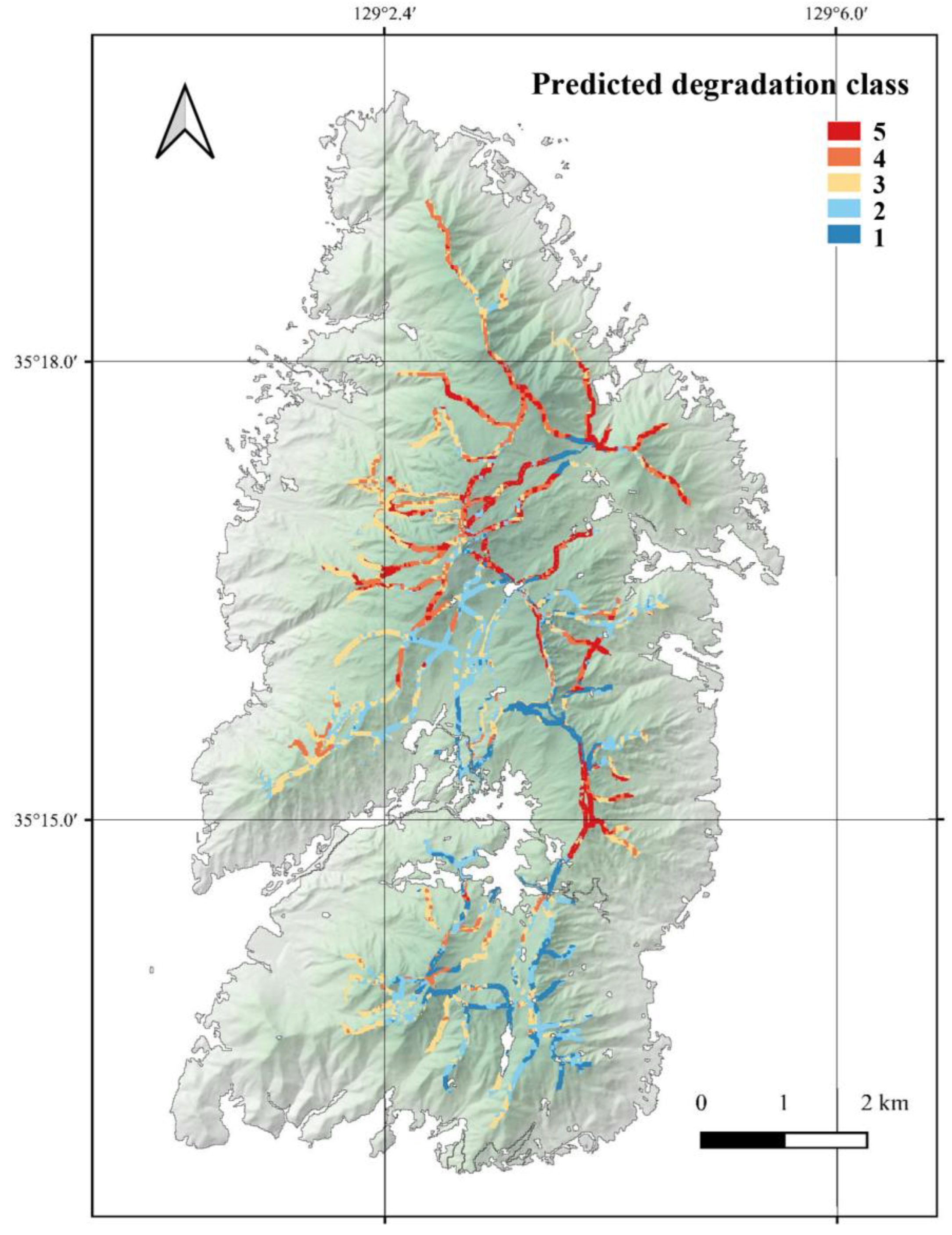
3.5. Trail Degradation Susceptibility Mapping

Trail degradation probability, as predicted by the RF model (ranging from 0 to 1), was visualized in a GIS environment to produce a trail degradation susceptibility map (Figure 4). This probability indicates the likelihood of degradation at each location, with higher values representing greater susceptibility. To systematically classify susceptibility levels, the Natural Breaks method was applied to the probability values, categorizing them into very low (0.00–0.32), low (0.32–0.48), moderate (0.48–0.61), high (0.61–0.74), and very high (0.74–0.95) degradation susceptibility.

Table 5. Statistical characteristics of variables by trail degradation class.

Variables		Predicted Degradation Class
		1	2	3	4	5
Pixel Count (%)		5883 (10.2%)	12,313 (21.3%)	16,060 (27.8%)	13,909 (24.1%)	9563 (16.6%)
Elevation (m)		494.9	450.6	466.4	495.0	513.4
TSA (Degrees)		48.4	51.2	43.1	38.2	44.9
TWI		8.6	8.7	9.0	9.6	10.2
LS		9.6	15.3	14.7	23.9	22.9
Aspect (Degrees)		158.1	177.2	200.7	206.2	215.7
NDVI		0.574	0.574	0.578	0.594	0.581
Slope (Degrees)		22.6	25.4	21.8	20.2	18.7
Vegetation Type	M (Mixed Forest of Conifers and Hardwoods)	5791	9013	6623	2727	1604
	D (Pine Forest)	-	999	2708	2299	1470
	H (Hardwood Forest)	-	1668	5086	6522	4931
	PR (Pinus rigida Forest)	-	4	405	793	1323
Soil Texture	R (Non-Forested area)	63	525	1028	1124	173
	SL (Sandy Loam)	2291	4313	5478	4495	4398
	L (Loam)	2106	4802	6510	6854	3979
	SiL (Silt Loam)	-	135	147	274	428

Note: Continuous variables (elevation, TSA, TWI, etc.) are presented as mean values, while categorical variables (vegetation type, soil texture) are represented by pixel count for each degradation class.

presents a comprehensive overview of the pixel distribution by susceptibility grade and the mean values of key environmental variables for each grade. It is noteworthy that the moderate susceptibility grade (grade 3) encompassed the most extensive area, accounting for 27.8% (16,060 pixels) of the study area. The combined grades 4 and 5 (high and very high susceptibility) accounted for 40.7% of the area, indicating that a significant portion of the study area is at a considerable susceptibility level of degradation. The remaining areas were classified as having very low (10.2%) and low (21.3%) susceptibility.

Continuous environmental variables manifested discernible patterns across susceptibility grades. For instance, elevation levels in areas classified as very low- to low-susceptibility ranged from an average of 450.6 to 494.9 m, whereas in high-susceptibility areas, they increased to 495.0–513.4 m, suggesting that elevated regions may be more susceptible to degradation. The TWI exhibited a consistent increase with higher susceptibility levels, ranging from 8.6 to 8.7 in very low- to low-susceptibility areas to 9.0 in moderate- and 9.6–10.2 in high-susceptibility areas, suggesting that areas with higher soil moisture are more vulnerable to erosion. Conversely, the LS Factor exhibited an increase from 9.6 to 15.3 in very low- to low-susceptibility areas to 22.9–23.9 in high-susceptibility areas. In contrast, slope reached its peak at grade 2 (25.4°) and decreased with increasing susceptibility, reaching 18.7° at grade 5. Aspect increased progressively with susceptibility, from an average of 158.1° in grade 1 to 215.7° in grade 5, suggesting that south- or southwest-facing slopes may be more vulnerable. The NDVI was slightly higher in high-susceptibility areas (0.581–0.594) compared to others, though differences were minimal. Conversely, TSA was found to be lower in moderate- to high-susceptibility areas compared to very low to low areas. This finding aligns with previous research that indicated that trails with lower TSA are more prone to degradation [61,68].

Categorical variables demonstrated significant variation across susceptibility grades. For instance, in very low- to low-susceptibility areas, mixed forests (M) predominated (98.4% and 73.2%, respectively), whereas in high-susceptibility areas, hardwood forests (H) were the most common (46.9% and 51.6%). In moderate-susceptibility areas, the distribution of mixed and hardwood forests was more balanced (41.2% and 31.7%, respectively), suggesting that hardwood forests may be more susceptible to degradation than mixed forests. Concerning soil texture, sandy loam (SL) was predominant in very low- to low-susceptibility areas (52.1% and 46.6%), while in high-susceptibility areas, loam (L) was dominant (59.1% and 41.6%). However, previous studies have reported that loam soils possess superior drainage properties [15,69]. Consequently, in the present study area, loam did not appear to be a significant factor influencing degradation prediction, as confirmed by the SHAP analysis.

4. Discussion

4.1. Explainable Prediction of Trail Degradation Susceptibility

This study successfully developed an environmental variable-based Random Forest model with SHAP interpretation for trail degradation prediction. The model achieved robust performance with an AUC-ROC of 0.812, and notably, spatial cross-validation revealed only a 10%–11% reduction (to 0.729). This minimal decrease, substantially lower than the 24%–30% typically reported in ecological modeling studies [67], suggests that our environmental predictors capture stable, generalizable patterns rather than site-specific anomalies.

The SHAP analysis revealed a hierarchical structure of environmental influences, providing quantitative insights into both the relative importance and directional effects of each predictor. Vegetation type emerged as the dominant control (mean absolute SHAP: 0.104), though its influence varied markedly by forest category. The low positive effect ratio (39.4%) reflects opposing effects within this categorical variable: hardwood forests and Pinus rigida plantations consistently produced positive SHAP values, indicating an association with higher degradation susceptibility, while mixed forests generated negative values, suggesting reduced susceptibility. This pattern challenges the assumptions of uniform vegetation effects and highlights the importance of species-specific management approaches.

The interpretation of variables with mean SHAP values of 0.000 (TWI, TSA, soil texture) requires careful consideration. Rather than indicating neutral effects, these balanced values reflect context-dependent behaviors. The TWI exemplifies this complexity with its 62.6% positive effect ratio—the variable shows protective associations at moderate moisture levels (TWI 8–9) where vegetation establishment is supported but contributes to degradation susceptibility at high values (TWI > 10) where soil saturation occurs. This threshold behavior suggests that simple linear assumptions about environmental influences may obscure critical tipping points in trail stability.

Elevation demonstrated consistent positive associations (52.5% positive effects) as the second most important variable, while soil texture, despite its modest importance score (0.030), showed the highest directional consistency (69.7% positive effects). This contrast between importance magnitude and effect consistency reveals that trail degradation results from both high-impact variables with variable effects and lower-impact variables with predictable influences—a nuance that traditional regression approaches might miss.

The spatial cross-validation performance warrants particular attention. The observed 10%–11% AUC reduction (0.812 to 0.729) falls substantially below the 24%–30% decrease typically reported in ecological modeling studies [67], suggesting that our environmental predictors capture relatively stable spatial patterns of trail degradation rather than localized anomalies.

4.2. Ecological Mechanisms and Theoretical Context

The dominance of vegetation type aligns with established knowledge of plant–soil interactions in disturbed environments. The susceptibility of hardwood forests and Pinus rigida plantations can be attributed to their root architecture characteristics. Studies have documented how hardwood species typically develop shallow, laterally extensive root systems optimized for nutrient acquisition [70], providing limited mechanical reinforcement against surface disturbance. Pinus rigida plantations, established as monocultures on previously degraded sites, lack the understory complexity and diverse root systems that characterize natural forest communities.

In contrast, mixed forests benefit from what Reubens et al. [71] describe as complementary soil reinforcement. The combination of deep coniferous taproots and dense deciduous fibrous networks creates overlapping reinforcement zones at multiple soil depths. This three-dimensional root architecture may explain the protective association observed in our SHAP analysis, as documented by Schwarz et al. [72], where root reinforcement is maximized in zones of overlapping root systems. The threshold behaviors observed in hydrological variables align with established geomorphological principles. The transition from protective to degradative influence at high TWI values reflects fundamental changes in soil mechanics—as pore water pressure increases, effective stress decreases, reducing shear strength below critical thresholds for stability [73]. Field observations of water accumulation and trail braiding in high-TWI zones corroborate these modeled relationships.

The success of environmental-only prediction in this anthropogenic system can be understood through the lens of recreational ecology theory. Marion et al. [63] documented asymptotic use–impact relationships where initial visitors cause disproportionate changes that stabilize over time. In mature trail systems like Geumjeongsan, experiencing decades of consistent use, environmental carrying capacity becomes the primary determinant of spatial degradation patterns after initial impacts reach equilibrium. Furthermore, the inherent correlation between trail routing and terrain favorability creates a natural coupling between environmental conditions and use intensity, validating our approach for practical applications.

4.3. Management Implications and Policy Integration

The trail degradation susceptibility map (Figure 5) provides empirical evidence for evaluating Geumjeongsan’s Restricted Access Policy, implemented since 1996 with rotating five-year closures across three management zones [31]. Overlay analysis revealed that Zone 2, where protection was lifted in 2021, exhibited the highest concentration of severe degradation (grades 4–5), affecting 34% of its area compared to 22% in Zone 1 and 18% in Zone 3. This disproportionate degradation in recently reopened areas suggests that the current rotation schedule may be insufficient for full ecological recovery. The spatial mismatch between administrative zones and environmental susceptibility patterns indicates opportunities for optimization. High-degradation susceptibility areas, comprising 40.7% of the total trail network, showed clustering along ridgelines and in hardwood-dominated sections, transcending current zone boundaries. This pattern suggests that management zones based solely on geographic divisions may not align with underlying environmental vulnerabilities, necessitating a shift toward environmentally informed zoning strategies consistent with science-based prioritization frameworks [74].

The integration of SHAP insights with susceptibility mapping enables targeted interventions across susceptibility categories. In very high-degradation susceptibility areas (16.6%), particularly hardwood forest sections with a TWI exceeding 10, the immediate installation of drainage systems and surface reinforcement is warranted. The importance of addressing hydrological issues aligns with findings that indicate that moisture accumulation accelerates trail degradation [75]. High-elevation trails above 600 m require seasonal closures during vulnerable periods, while Pinus rigida plantation trails need priority surface stabilization given their documented susceptibility in monoculture systems [76].

The environmental variable-based approach offers significant operational advantages for resource-limited management contexts. The model’s scalability allows for application to unmapped trail sections using readily available GIS data, eliminating the need for expensive visitor monitoring infrastructure. By identifying future degradation susceptibility areas before visible degradation occurs, managers can shift from reactive to proactive strategies. This predictive approach is particularly valuable given the asymptotic nature of trail impacts, where initial damage occurs rapidly before stabilizing [63].

Beyond immediate applications, the susceptibility map serves as a decision support tool for long-term trail planning, maintenance scheduling, and budget allocation. Forest managers can prioritize interventions based on environmental susceptibility rather than responding to degradation after it occurs. The integration of environmental variables with spatial analysis has proven effective for trail assessment in various protected areas [25]. This predictive capacity is particularly valuable given increasing recreational pressure and climate variability, which may alter historical degradation patterns. The framework’s reliance on standard environmental datasets ensures transferability to other forest systems facing similar management challenges, offering a practical solution for the many protected areas worldwide that lack comprehensive visitor monitoring programs.

4.4. Limitations and Future Research

While this study demonstrates the viability of environmental-only prediction for trail degradation assessment, several limitations should be acknowledged. The binary classification of trail conditions, though operationally practical, may oversimplify the continuous nature of degradation processes. Future research could benefit from developing automated landscape assessment techniques to quantify trail conditions more objectively, potentially using UAV-based photogrammetry or computer vision approaches for continuous degradation metrics [59].

The sampling design encompassing 142 points across approximately 16% of the trail network provided reasonable spatial coverage but may not capture all local variations. Although spatial cross-validation showed robust performance, external validation in different forest systems would strengthen model transferability claims [21]. The relatively coarse resolution of environmental data (10 m DEM and 1:25,000 scale maps) proved adequate for landscape-level predictions, yet finer-scale data could reveal important microtopographic influences on trail degradation patterns [24].

Future research directions should explore several promising avenues. The integration of high-resolution remote sensing data, particularly LiDAR-derived terrain metrics, could enhance the detection of subtle topographic features influencing water flow and erosion [8]. Multi-temporal satellite imagery analysis would enable the monitoring of vegetation dynamics and their relationship with trail stability [22]. At the methodological level, ensemble approaches combining multiple algorithms could improve prediction reliability by leveraging the strengths of different modeling techniques [25].

The limited availability of comprehensive trail degradation datasets currently constrains the application of more complex modeling approaches. However, as monitoring data accumulates through continued field efforts and automated assessment techniques, opportunities will emerge for developing interdisciplinary research frameworks that integrate ecological, geomorphological, and recreational perspectives [15]. Such frameworks could incorporate diverse data sources and analytical methods to create a more nuanced understanding of trail system dynamics.

The absence of visitor use data, while limiting certain analyses, paradoxically enhances the practical applicability of our approach given that most forest management agencies face similar constraints [9]. The future development of hybrid models that opportunistically incorporate available use data while maintaining the environmental baseline would provide flexible solutions adaptable to varying data availability contexts. The current framework demonstrates that robust predictive performance (AUC-ROC = 0.812) can be achieved using readily available environmental datasets, thereby providing an operational solution for trail management in the absence of comprehensive visitor monitoring infrastructure.

5. Conclusions

This study established a practical framework for proactive trail management in data-constrained environments by demonstrating that environmental variables alone can effectively predict degradation susceptibility. The integration of Random Forest modeling with SHAP interpretation not only achieved robust predictive performance (AUC-ROC = 0.812) but also provided mechanistic insights into the complex interactions between environmental factors and trail stability.

This research revealed nuanced patterns of environmental controls on trail degradation. While vegetation type emerged as the dominant predictor, its effects varied substantially by forest composition, challenging the assumptions of uniform vegetation influences. The threshold behaviors observed in hydrological variables, particularly the TWI’s transition from protective to degradative effects at high moisture levels, underscore the non-linear nature of trail degradation processes. These findings suggest that effective trail management requires an understanding of critical environmental tipping points rather than simple linear relationships.

Based on these insights, we propose the following management strategies. First, priority interventions should target the 40.7% of trail networks classified as high- to very high-susceptibility, with particular attention paid to hardwood forest sections where the TWI exceeds 10. Second, immediate surface reinforcement is recommended for the 16.6% of areas with very high degradation risk. Third, seasonal closures should be considered for high-elevation trails above 600 m during vulnerable periods. Fourth, Pinus rigida plantation trails warrant prioritized stabilization efforts given their documented susceptibility in monoculture systems.

The absence of visitor use data, while limiting certain analyses, paradoxically enhances the practical applicability of our approach given that most forest management agencies face similar constraints. This research contributes to the broader goal of balancing recreational access with ecological integrity in forest ecosystems. By providing a practical, evidence-based approach to trail susceptibility assessment, this study supports proactive management strategies that respond to both immediate management needs and long-term sustainability challenges.

References

1. Tomczyk, A.M. A GIS Assessment and Modelling of Environmental Sensitivity of Recreational Trails: The Case of Gorce National Park, Poland. Appl. Geogr. 2011, 31, 339–351. [Google Scholar] [CrossRef]
2. Pagneux, E.; Sturludóttir, E.; Ólafsdóttir, R. Modelling of Recreational Trails in Mountainous Areas: An Analysis of Sensitivity to Slope Data Resolution. Appl. Geogr. 2023, 160, 103112. [Google Scholar] [CrossRef]
3. Venter, Z.S.; Barton, D.N.; Gundersen, V.; Figari, H.; Nowell, M.S. Back to Nature: Norwegians Sustain Increased Recreational Use of Urban Green Space Months after the COVID-19 Outbreak. Landsc. Urban. Plan. 2021, 214, 104175. [Google Scholar] [CrossRef]
4. Spernbauer, B.S.; Monz, C.; D’Antonio, A.; Smith, J.W. Factors Influencing Informal Trail Conditions: Implications for Management and Research in Urban-Proximate Parks and Protected Areas. Landsc. Urban. Plan. 2023, 231, 104661. [Google Scholar] [CrossRef]
5. Alice, L.; Ivana, Z.; Jerylee, W.A. Mountain Bike Trails in Urban Forests: Meeting Recreation Demands in Vienna and Zurich. J. Outdoor Recreat. Tour. 2025, 49, 100861. [Google Scholar] [CrossRef]
6. Ballantyne, M.; Pickering, C.M. The Impacts of Trail Infrastructure on Vegetation and Soils: Current Literature and Future Directions. J. Environ. Manag. 2015, 164, 53–64. [Google Scholar] [CrossRef]
7. Hockett, K.S.; Marion, J.L.; Leung, Y.F. The Efficacy of Combined Educational and Site Management Actions in Reducing Off-Trail Hiking in an Urban-Proximate Protected Area. J. Environ. Manag. 2017, 203, 17–28. [Google Scholar] [CrossRef]
8. Chisholm, T.; McCune, J.L. Vegetation Type and Trail Use Interact to Affect the Magnitude and Extent of Recreational Trail Impacts on Plant Communities. J. Environ. Manag. 2024, 351, 119817. [Google Scholar] [CrossRef]
9. Power, D.; Lambe, B.; Murphy, N. Trends in Recreational Walking Trail Usage in Ireland during the COVID-19 Pandemic: Implications for Practice. J. Outdoor Recreat. Tour. 2023, 41, 100477. [Google Scholar] [CrossRef]
10. Misra, S.; Abdelgawad, N.; Wernstedt, K.; Saaty, M.; Patel, J.; Marion, J.; McCrickard, S. Toward a Management Framework for Smart and Sustainable Resource Management: The Case of the Appalachian Trail. J. Environ. Manag. 2024, 372, 123422. [Google Scholar] [CrossRef]
11. Rodway-Dyer, S.; Ellis, N. Combining Remote Sensing and On-Site Monitoring Methods to Investigate Footpath Erosion within a Popular Recreational Heathland Environment. J. Environ. Manag. 2018, 215, 68–78. [Google Scholar] [CrossRef] [PubMed]
12. Peterson, B.A.; Brownlee, M.T.J.; Marion, J.L. Mapping the Relationships between Trail Conditions and Experiential Elements of Long-Distance Hiking. Landsc. Urban. Plan. 2018, 180, 60–75. [Google Scholar] [CrossRef]
13. Cole, D.N. Minimizing Conflict between Recreation and Nature Conservation. In Ecology of Greenways: Design and Function of Linear Conservation Areas; University of Minnesota Press: Minneapolis, MN, USA, 1993; pp. 105–122. [Google Scholar]
14. Leung, Y.-F.; Marion, J.L. Trail Degradation as Influenced by Environmental Factors: A State-of-the-Knowledge Review. J. Soil. Water Conserv. 1996, 51, 130–136. [Google Scholar] [CrossRef]
15. Marion, J.L. Trail Sustainability: A State-of-Knowledge Review of Trail Impacts, Influential Factors, Sustainability Ratings, and Planning and Management Guidance. J. Environ. Manag. 2023, 340, 117868. [Google Scholar] [CrossRef]
16. Tomczyk, A.M.; Ewertowski, M. Planning of Recreational Trails in Protected Areas: Application of Regression Tree Analysis and Geographic Information Systems. Appl. Geogr. 2013, 40, 129–139. [Google Scholar] [CrossRef]
17. Salesa, D.; Cerdà, A. Soil Erosion on Mountain Trails as a Consequence of Recreational Activities. A Comprehensive Review of the Scientific Literature. J. Environ. Manag. 2020, 271, 110990. [Google Scholar] [CrossRef] [PubMed]
18. dos Santos Pereira, L.; Rodrigues, A.M.; do Carmo Oliveira Jorge, M.; Guerra, A.J.T.; Booth, C.A.; Fullen, M.A. Detrimental Effects of Tourist Trails on Soil System Dynamics in Ubatuba Municipality, São Paulo State, Brazil. Catena 2022, 216, 106431. [Google Scholar] [CrossRef]
19. Marion, J.L.; Olive, N. Assessing and Understanding Trail Degradation: Results from Big South Fork National River and Recreational Area; U.S. Geological Survey: Reston, VA, USA, 2006. [CrossRef]
20. Hammitt, W.E.; Cole, D.N.; Monz, C.A. Wildland Recreation: Ecology and Management; John Wiley & Sons: Hoboken, NJ, USA, 2015. [Google Scholar]
21. Minehart, K.; Antonio, A.D.; Creany, N.; Monz, C.; Gutzwiller, K. Predicting Trail Condition Using Random Forest Models in Urban-Proximate Nature Reserves. Environ. Chall. 2024, 15, 100937. [Google Scholar] [CrossRef]
22. Hilyer, T.; Martin, R.H.; Turley, F. Comparing Hydrologic Impacts on Recreational Trails to Remotely Sensed Data. Remote Sens. Appl. 2023, 32, 101052. [Google Scholar] [CrossRef]
23. Tomczyk, A.M.; Ewertowski, M.W. Recreational Trails in the Poprad Landscape Park, Poland: The Spatial Pattern of Trail Impacts and Use-Related, Environmental, and Managerial Factors. J. Maps 2016, 12, 1227–1235. [Google Scholar] [CrossRef]
24. Eagleston, H.; Marion, J.L. Application of Airborne LiDAR and GIS in Modeling Trail Erosion along the Appalachian Trail in New Hampshire, USA. Landsc. Urban. Plan. 2020, 198, 103765. [Google Scholar] [CrossRef]
25. Sahani, N.; Ghosh, T. GIS-Based Spatial Prediction of Recreational Trail Susceptibility in Protected Area of Sikkim Himalaya Using Logistic Regression, Decision Tree and Random Forest Model. Ecol. Inform. 2021, 64, 101352. [Google Scholar] [CrossRef]
26. Buchelt, A.; Adrowitzer, A.; Kieseberg, P.; Gollob, C.; Nothdurft, A.; Eresheim, S.; Tschiatschek, S.; Stampfer, K.; Holzinger, A. Exploring Artificial Intelligence for Applications of Drones in Forest Ecology and Management. For. Ecol. Manag. 2024, 551, 121530. [Google Scholar] [CrossRef]
27. Peng, C.-Y.J.; Lee, K.L.; Ingersoll, G.M. An Introduction to Logistic Regression Analysis and Reporting. J. Educ. Res. 2002, 96, 3–14. [Google Scholar] [CrossRef]
28. Lee, S.; Sambath, T. Landslide Susceptibility Mapping in the Damrei Romel Area, Cambodia Using Frequency Ratio and Logistic Regression Models. Environ. Geol. 2006, 50, 847–855. [Google Scholar] [CrossRef]
29. Korea Forest Service Website. Available online: https://kfss.forest.go.kr/stat/ptl/main/main.do?CSRFToken=null (accessed on 7 May 2025).
30. Korea Meteorological Administration Website. Available online: https://www.weather.go.kr/w/index.do (accessed on 7 May 2025).
31. Busan City. 2024. Available online: https://www.busan.go.kr/eng/index (accessed on 7 May 2025).
32. Yeo, W.-S. Promotion Tasks for the Designation of Geumjeongsan as a National Park in Busan; Busan Development Institute: 2019. Available online: https://www.dbpia.co.kr/journal/articleDetail?nodeId=NODE09228542 (accessed on 7 May 2025).
33. Ministry of Environment Website (Land Cover Maps). Available online: https://www.me.go.kr/home/web/main.do (accessed on 7 May 2025).
34. Marquet, O.; Mojica, L.; Fernández-Núñez, M.-B.; Maciejewska, M. Pathways to 15-Minute City Adoption: Can Our Understanding of Climate Policies’ Acceptability Explain the Backlash towards x-Minute City Programs? Cities 2024, 148, 104878. [Google Scholar] [CrossRef]
35. Bruehler, G.; Sondergaard, M. GIS/GPS Trail Condition Inventories: A Virtual Toolbox for Trail Managers. In Proceedings of the Twenty-Fourth Annual ESRI User Conference, San Diego, CA, USA, 14–18 July 2004; pp. 9–13. [Google Scholar]
36. Leung, Y.-F.; Marion, J.L. The Influence of Sampling Interval on the Accuracy of Trail Impact Assessment. Landsc. Urban. Plan. 1999, 43, 167–179. [Google Scholar] [CrossRef]
37. Monz, C.A.; Marion, J.L.; Goonan, K.A.; Manning, R.E.; Wimpey, J.; Carr, C. Assessment and Monitoring of Recreation Impacts and Resource Conditions on Mountain Summits: Examples From the Northern Forest, USA. Mt. Res. Dev. 2010, 30, 332–343. [Google Scholar] [CrossRef]
38. Nepal, S.K. Trail Impacts in Sagarmatha (Mt. Everest) National Park, Nepal: A Logistic Regression Analysis. Environ. Manag. 2003, 32, 312–321. [Google Scholar] [CrossRef]
39. QGIS Development Team. QGIS Geographic Information System, Version 3.34; Open Source Geospatial Foundation Project: Beaverton, OR, USA, 2024; Available online: https://qgis.org (accessed on 7 May 2025).
40. Neter, J.; Kutner, M.H.; Nachtsheim, C.J.; Wasserman, W. Applied Linear Statistical Models; Irwin Professional Publishing: Burr Ridge, IL, USA, 1996. [Google Scholar]
41. Breiman, L. Random Forests. Mach. Learn. 2001, 45, 5–32. [Google Scholar] [CrossRef]
42. Shapley, L.S. A Value for N-Person Games. Contrib. Theory Games 1953, 2, 307–317. [Google Scholar]
43. Lundberg, S.M.; Lee, S.-I. A Unified Approach to Interpreting Model Predictions. Adv. Neural Inf. Process Syst. 2017, 30, 4768–4777. [Google Scholar]
44. Kim, H.; Kim, D. Changes in Urban Growth Patterns in Busan Metropolitan City, Korea: Population and Urbanized Areas. Land 2022, 11, 1319. [Google Scholar] [CrossRef]
45. Bai, W.-P.; Cheng, S.-Q.; Guo, X.-Y.; Wang, Y.; Guo, Q.; Tan, C.-D. Oilfield Analogy and Productivity Prediction Based on Machine Learning: Field Cases in PL Oilfield, China. Pet. Sci. 2024, 21, 2554–2570. [Google Scholar] [CrossRef]
46. Ding, X.; Feng, B.; Wu, J. The Influence of Two and Three-Dimensional Spatial Characteristics of Industrial Parks on the Emotional Well-Being of Employees: A Case Study of Shenzhen. Appl. Geogr. 2024, 171, 103367. [Google Scholar] [CrossRef]
47. Abdulrashid, I.; Chiang, W.-C.; Sheu, J.-B.; Mammadov, S. An Interpretable Machine Learning Framework for Enhancing Road Transportation Safety. Transp. Res. E Logist. Transp. Rev. 2025, 195, 103969. [Google Scholar] [CrossRef]
48. El Mokhtari, K.; Higdon, B.P.; Başar, A. Interpreting Financial Time Series with SHAP Values. In Proceedings of the 29th Annual International Conference on Computer Science and Software Engineering, Markham, ON, Canada, 4–6 November 2019; pp. 166–172. [Google Scholar]
49. Lombardo, L.; Cama, M.; Conoscenti, C.; Märker, M.; Rotigliano, E. Binary Logistic Regression versus Stochastic Gradient Boosted Decision Trees in Assessing Landslide Susceptibility for Multiple-Occurring Landslide Events: Application to the 2009 Storm Event in Messina (Sicily, Southern Italy). Nat. Hazards 2015, 79, 1621–1648. [Google Scholar] [CrossRef]
50. Ding, C.; Wang, D.; Ma, X.; Li, H. Predicting Short-Term Subway Ridership and Prioritizing Its Influential Factors Using Gradient Boosting Decision Trees. Sustainability 2016, 8, 1100. [Google Scholar] [CrossRef]
51. Sachdeva, S.; Bhatia, T.; Verma, A.K. GIS-Based Evolutionary Optimized Gradient Boosted Decision Trees for Forest Fire Susceptibility Mapping. Nat. Hazards 2018, 92, 1399–1418. [Google Scholar] [CrossRef]
52. Cohen, J. A Coefficient of Agreement for Nominal Scales. Educ. Psychol. Meas. 1960, 20, 37–46. [Google Scholar] [CrossRef]
53. Louppe, G.; Wehenkel, L.; Sutera, A.; Geurts, P. Understanding Variable Importances in Forests of Randomized Trees. Adv. Neural Inf. Process Syst. 2013, 26, 431–439. [Google Scholar]
54. Hassan, S.U.; Ahamed, J.; Ahmad, K. Analytics of Machine Learning-Based Algorithms for Text Classification. Sustain. Oper. Comput. 2022, 3, 238–248. [Google Scholar] [CrossRef]
55. Valero-Carreras, D.; Alcaraz, J.; Landete, M. Comparing Two SVM Models through Different Metrics Based on the Confusion Matrix. Comput. Oper. Res. 2023, 152, 106131. [Google Scholar] [CrossRef]
56. Phillips, G.; Teixeira, H.; Kelly, M.G.; Salas Herrero, F.; Várbíró, G.; Lyche Solheim, A.; Kolada, A.; Free, G.; Poikane, S. Setting Nutrient Boundaries to Protect Aquatic Communities: The Importance of Comparing Observed and Predicted Classifications Using Measures Derived from a Confusion Matrix. Sci. Total Environ. 2024, 912, 168872. [Google Scholar] [CrossRef] [PubMed]
57. Roberts, D.R.; Bahn, V.; Ciuti, S.; Boyce, M.S.; Elith, J.; Guillera-Arroita, G.; Hauenstein, S.; Lahoz-Monfort, J.J.; Schröder, B.; Thuiller, W.; et al. Cross-Validation Strategies for Data with Temporal, Spatial, Hierarchical, or Phylogenetic Structure. Ecography 2017, 40, 913–929. [Google Scholar] [CrossRef]
58. Valavi, R.; Elith, J.; Lahoz-Monfort, J.J.; Guillera-Arroita, G. BlockCV: An r Package for Generating Spatially or Environmentally Separated Folds for k-Fold Cross-Validation of Species Distribution Models. Methods Ecol. Evol. 2019, 10, 225–232. [Google Scholar] [CrossRef]
59. Tomczyk, A.M.; Ewertowski, M.W.; Creany, N.; Ancin-Murguzur, F.J.; Monz, C. The Application of Unmanned Aerial Vehicle (UAV) Surveys and GIS to the Analysis and Monitoring of Recreational Trail Conditions. Int. J. Appl. Earth Obs. Geoinf. 2023, 123, 103474. [Google Scholar] [CrossRef]
60. Evju, M.; Hagen, D.; Jokerud, M.; Olsen, S.L.; Selvaag, S.K.; Vistad, O.I. Effects of Mountain Biking versus Hiking on Trails under Different Environmental Conditions. J. Environ. Manag. 2021, 278, 111554. [Google Scholar] [CrossRef]
61. Meadema, F.; Marion, J.L.; Arredondo, J.; Wimpey, J. The Influence of Layout on Appalachian Trail Soil Loss, Widening, and Muddiness: Implications for Sustainable Trail Design and Management. J. Environ. Manag. 2020, 257, 109986. [Google Scholar] [CrossRef]
62. Bodoque, J.M.; Ballesteros-Cánovas, J.A.; Rubiales, J.M.; Perucha, M.Á.; Nadal-Romero, E.; Stoffel, M. Quantifying Soil Erosion from Hiking Trail in a Protected Natural Area in the Spanish Pyrenees. Land. Degrad. Dev. 2017, 28, 2255–2267. [Google Scholar] [CrossRef]
63. Marion, J.L. A Review and Synthesis of Recreation Ecology Research Supporting Carrying Capacity and Visitor Use Management Decisionmaking. J. For. 2016, 114, 339–351. [Google Scholar] [CrossRef]
64. Olive, N.D.; Marion, J.L. The Influence of Use-Related, Environmental, and Managerial Factors on Soil Loss from Recreational Trails. J. Environ. Manag. 2009, 90, 1483–1493. [Google Scholar] [CrossRef]
65. Hosmer Jr, D.W.; Lemeshow, S.; Sturdivant, R.X. Applied Logistic Regression; John Wiley & Sons: Hoboken, NJ, USA, 2013. [Google Scholar]
66. Park, S.; Kim, J. Landslide Susceptibility Mapping Based on Random Forest and Boosted Regression Tree Models, and a Comparison of Their Performance. Appl. Sci. 2019, 9, 942. [Google Scholar] [CrossRef]
67. Schratz, P.; Muenchow, J.; Iturritxa, E.; Richter, J.; Brenning, A. Hyperparameter Tuning and Performance Assessment of Statistical and Machine-Learning Algorithms Using Spatial Data. Ecol. Modell. 2019, 406, 109–120. [Google Scholar] [CrossRef]
68. Marion, J.L.; Wimpey, J. Assessing the Influence of Sustainable Trail Design and Maintenance on Soil Loss. J. Environ. Manag. 2017, 189, 46–57. [Google Scholar] [CrossRef]
69. Parker, T.S. Natural Surface Trails by Design: Physical and Human Design Essentials of Sustainable, Enjoyable Trails; Natureshape: Fatehpur, India, 2004. [Google Scholar]
70. De Baets, S.; Poesen, J.; Reubens, B.; Wemans, K.; De Baerdemaeker, J.; Muys, B. Root Tensile Strength and Root Distribution of Typical Mediterranean Plant Species and Their Contribution to Soil Shear Strength. Plant Soil. 2008, 305, 207–226. [Google Scholar] [CrossRef]
71. Reubens, B.; Poesen, J.; Danjon, F.; Geudens, G.; Muys, B. The Role of Fine and Coarse Roots in Shallow Slope Stability and Soil Erosion Control with a Focus on Root System Architecture: A Review. Trees-Struct. Funct. 2007, 21, 385–402. [Google Scholar] [CrossRef]
72. Schwarz, M.; Lehmann, P.; Or, D. Quantifying Lateral Root Reinforcement in Steep Slopes—From a Bundle of Roots to Tree Stands. Earth Surf. Process Landf. 2010, 35, 354–367. [Google Scholar] [CrossRef]
73. Kemppinen, J.; Niittynen, P.; Riihimäki, H.; Luoto, M. Modelling Soil Moisture in a High-Latitude Landscape Using LiDAR and Soil Data. Earth Surf. Process Landf. 2018, 43, 1019–1031. [Google Scholar] [CrossRef]
74. Tomczyk, A.M.; Ewertowski, M.W.; White, P.C.L.; Kasprzak, L. A New Framework for Prioritising Decisions on Recreational Trail Management. Landsc. Urban. Plan. 2017, 167, 1–13. [Google Scholar] [CrossRef]
75. Seutloali, K.E.; Dube, T.; Mutanga, O. Assessing and Mapping the Severity of Soil Erosion Using the 30-m Landsat Multispectral Satellite Data in the Former South African Homelands of Transkei. Phys. Chem. Earth Parts A/B/C 2017, 100, 296–304. [Google Scholar] [CrossRef]
76. Liu, M.; Zhang, D.; Pietzarka, U.; Roloff, A. Assessing the Adaptability of Urban Tree Species to Climate Change Impacts: A Case Study in Shanghai. Urban. For. Urban. Green. 2021, 62, 127186. [Google Scholar] [CrossRef]
77. National Geographic Information Institute. National Geographic Information Institute Website. Available online: https://www.ngii.go.kr (accessed on 7 May 2025).
78. Ólafsdóttir, R.; Runnström, M.C. Assessing Hiking Trails Condition in Two Popular Tourist Destinations in the Icelandic Highlands. J. Outdoor Recreat. Tour. 2013, 3–4, 57–67. [Google Scholar] [CrossRef]
79. Pal, S.; Debanshi, S. Influences of Soil Erosion Susceptibility toward Overloading Vulnerability of the Gully Head Bundhs in Mayurakshi River Basin of Eastern Chottanagpur Plateau. Environ. Dev. Sustain. 2018, 20, 1739–1775. [Google Scholar] [CrossRef]
80. Marion, J.L.; Wimpey, J. Informal Trail Monitoring Protocols: Denali National Park and Preserve. Usgs 2011, 76. [Google Scholar] [CrossRef]
81. Datta, P.S.; Schack-Kirchner, H. Erosion Relevant Topographical Parameters Derived from Different DEMs—A Comparative Study from the Indian Lesser Himalayas. Remote Sens. 2010, 2, 1941–1961. [Google Scholar] [CrossRef]
82. Korea Forest Service. Korea Forest Service Website. Available online: https://www.forest.go.kr/kfsweb/kfs/idx/Index.do (accessed on 7 May 2025).
83. Bratton, S.P.; Hickler, M.G.; Graves, J.H. Trail Erosion Patterns in Great Smoky Mountains National Park. Environ. Manag. 1979, 3, 431–445. [Google Scholar] [CrossRef]
84. Hall, C.N.; Kuss, F.R. Vegetation Alteration along Trails in Shenandoah National Park, Virginia. Biol. Conserv. 1989, 48, 211–227. [Google Scholar] [CrossRef]
85. European Space Agency. Sentinel-2 Satellite Imagery. Available online: https://browser.dataspace.copernicus.eu/ (accessed on 7 May 2025).
86. Kim, H.W.; Kim, J.H.; Li, W.; Yang, P.; Cao, Y. Exploring the Impact of Green Space Health on Runoff Reduction Using NDVI. Urban For Urban Green 2017, 28, 81–87. [Google Scholar] [CrossRef]
87. Liu, C.; White, M.; Newell, G. Measuring and Comparing the Accuracy of Species Distribution Models with Presence–Absence Data. Ecography 2011, 34, 232–243. [Google Scholar] [CrossRef]
88. Finley, J.P. Tornado Predictions. Am. Meteorol. J. A Mon. Rev. Meteorol. Allied Branches Study (1884–1896) 1884, 1, 85. [Google Scholar]
89. Fielding, A.H.; Bell, J.F. A Review of Methods for the Assessment of Prediction Errors in Conservation Presence/Absence Models. Environ. Conserv. 1997, 24, 38–49. [Google Scholar] [CrossRef]
90. Daskalaki, S.; Kopanas, I.; Avouris, N. Evaluation of Classifiers for an Uneven Class Distribution Problem. Appl. Artif. Intell. 2006, 20, 381–417. [Google Scholar] [CrossRef]
91. Bradley, A.P. The Use of the Area under the ROC Curve in the Evaluation of Machine Learning Algorithms. Pattern Recognit. 1997, 30, 1145–1159. [Google Scholar] [CrossRef]
Figure 1. Location and trail network of Geumjeongsan, Busan. (a) Geographical location of the study area within South Korea. (b) Administrative boundary and elevation of Geumjeongsan Mountain in Busan. (c) Land cover classification in the study area with trail network, Godangbong Peak, and field survey points.
Forests 16 01074 g001
Figure 2. The framework for this study.
Forests 16 01074 g002
Figure 3. Trail conditions observed during field survey. (a) Water accumulation in center of trail due to poor natural drainage. (b) Trail widening caused by presence of small rocks, leading hikers to seek alternative paths. (c) Severe soil erosion and vegetation loss along trail edges, causing land degradation. (d) Trail with extensive root and rock exposure, making surface uneven and difficult to traverse. (e) Trail incision due to soil erosion, leading to trail braiding and expansion. (f) Stable trail with appropriate bare soil exposure and dense surrounding vegetation. (g) Stable trail with appropriate bare soil exposure and dense surrounding vegetation. (h) Severe soil erosion alongside trail, creating deep hollow near path. (i) Stable trail with appropriate bare soil exposure and dense surrounding vegetation.
Forests 16 01074 g003
Figure 4. Trail degradation susceptibility map based on RF model.
Forests 16 01074 g004
Figure 5. Comparison of trail degradation susceptibility with restricted access zones.
Forests 16 01074 g005