Ecosystem Service Synergies and Trade-Offs in Poplar–Birch Mixed Natural Forests Across Different Developmental Stages

Abstract

Forest ecosystem services are crucial for sustaining ecological balance and supporting human well-being. This study quantified and analyzed ecosystem services—carbon storage, water conservation, and productivity—across four developmental stages (I, II, III, and IV) of poplar (Populus davidiana)–birch (Betula platyphylla) mixed natural secondary forests (MPB) in Weichang County, China, over the year 2022 using the InVEST and biomass models. Synergies and trade-offs between these ecosystem services were assessed using the constraint line method. The results showed that as the stand developed, carbon storage values gradually increased, while productivity remained relatively low during the initial three stages but exhibited a significant upward trend by Stage IV (p < 0.05). In contrast, water conservation did not exhibit a clear pattern with stand development. Across all stages, carbon storage exhibited a synergistic relationship with productivity, but a trade-off was observed with water conservation. In the first three stages, productivity and water conservation were in trade-off, yet by Stage IV, this relationship shifted to a weak synergy. The constraint line analysis revealed dynamic trade-offs between productivity, carbon storage, and water conservation. The findings emphasize the importance of adopting adaptive management strategies for MPB at different developmental stages to maximize the synergistic effects among ecosystem services.

1. Introduction

Ecosystem services (ESs) are essential goods and services provided by natural ecosystems, crucial for human well-being. These services are indispensable for maintaining ecological balance and ensuring human welfare [1]. Functions such as carbon storage, water conservation, and productivity are vital for mitigating climate change [2], supplying timber and other forest products [3], and sustaining the water cycle [4,5]. Natural forests, compared to other land cover types, offer a greater diversity of ESs [6]. Therefore, understanding the intrinsic value of natural forests and implementing optimal ecosystem management are crucial for enhancing their overall function and value.

Interactions among forest ESs often result in synergies or trade-offs due to their interconnected nature [7]. Trade-offs often involve enhancing one service at the expense of another. For instance, Swedish forest management strategies aimed at increasing timber production for bioenergy and bioeconomic goals may compromise forest multifunctionality [8]. Although intensive harvesting increases timber supply, it reduces the forest’s capacity for carbon storage and biodiversity conservation. Conversely, synergy among ESs occurs when two or more services reinforce each other. In German forests, nature conservation and biomass production strategies are employed to adapt to climate change. These strategies have been shown to enhance long-term carbon storage and biodiversity, thereby partially balancing the synergy between carbon storage and productivity [9]. Similarly, sustainable forest management in Finland has demonstrated that protective measures can simultaneously enhance carbon sequestration and water retention by reducing evapotranspiration and enhancing soil moisture availability [10]. Additionally, forest ecosystems rich in biodiversity not only offer effective disease control but also contribute to soil fertility and water retention through the activities of healthy microbial communities, stabilizing water resources [11]. Despite the increasing focus on the relationships between ESs, most studies have concentrated on specific watersheds [12,13] administrative regions [14], or land use types [13,15]. However, limited attention has been paid to the ecological characteristics of forests at different developmental stages and their impact on ecosystem services. Addressing this gap requires examining ESs in a developmental context to inform effective management practices.

In this study, the InVEST model was used to quantify ESs. The model’s modular design offers adaptability and precision for evaluating the impacts of different land-use and management strategies on ESs across various regions [16]. Researchers often employ various methods to assess trade-offs and synergies among ESs. While statistical techniques such as Pearson’s or Spearman’s correlation analysis are effective for identifying linear relationships, they often fail to capture non-linear interactions [17]. Spatial analysis offers clear visualization of ES distribution but is constrained by data availability and resolution [18]. Scenario modeling is another approach used to predict the potential effects of various management strategies but depends heavily on the validity of the underlying assumptions [19]. The interactions between ESs are often non-linear and influenced by multiple environmental factors [20]. The constraint line approach effectively identifies trade-off zones and synergistic areas by mapping boundaries between services, offering insights into non-linear interactions [21,22]. In this study, the constraint line method was selected to examine the synergistic and trade-off relationships among ESs in poplar (Populus davidiana)–birch (Betula platyphylla) mixed natural secondary forests (MPB) across different developmental stages.

Historically, the Saihanba area in northern Hebei, China, served as a royal hunting ground. However, significant ecological degradation occurred in the early 1900s due to human activities. Since 1962, a large-scale afforestation initiative has been implemented, transforming the ecosystem into a near-natural state. These efforts included planting needleleaf tree species such as larch (Larix principis-rupprechtii) and spruce (Picea asperata), as well as broadleaf species like white birch and Mongolian oak (Quercus mongolica) [23]. According to the Ninth National Forest Inventory, MPB at various developmental stages now comprise 41.24% of the total forest area in the region. These secondary forests play a crucial role in providing key ESs. Their extensive distribution and diverse ESs are indispensable for preserving regional ecological equilibrium and supporting the sustainable development of local communities [24]. Given the importance of these forests, a quantitative assessment of ESs for MPB at different developmental stages is essential.

This study aimed to (1) quantify the productivity, carbon storage, and water conservation services of MPB across developmental stages, and (2) investigate the trade-offs and synergies among ESs and elucidate the constraining effects among these services. By addressing these objectives, the study seeks to advance understanding of ES interactions at different developmental stages, contributing to landscape optimization and the development of multifunctional management strategies.

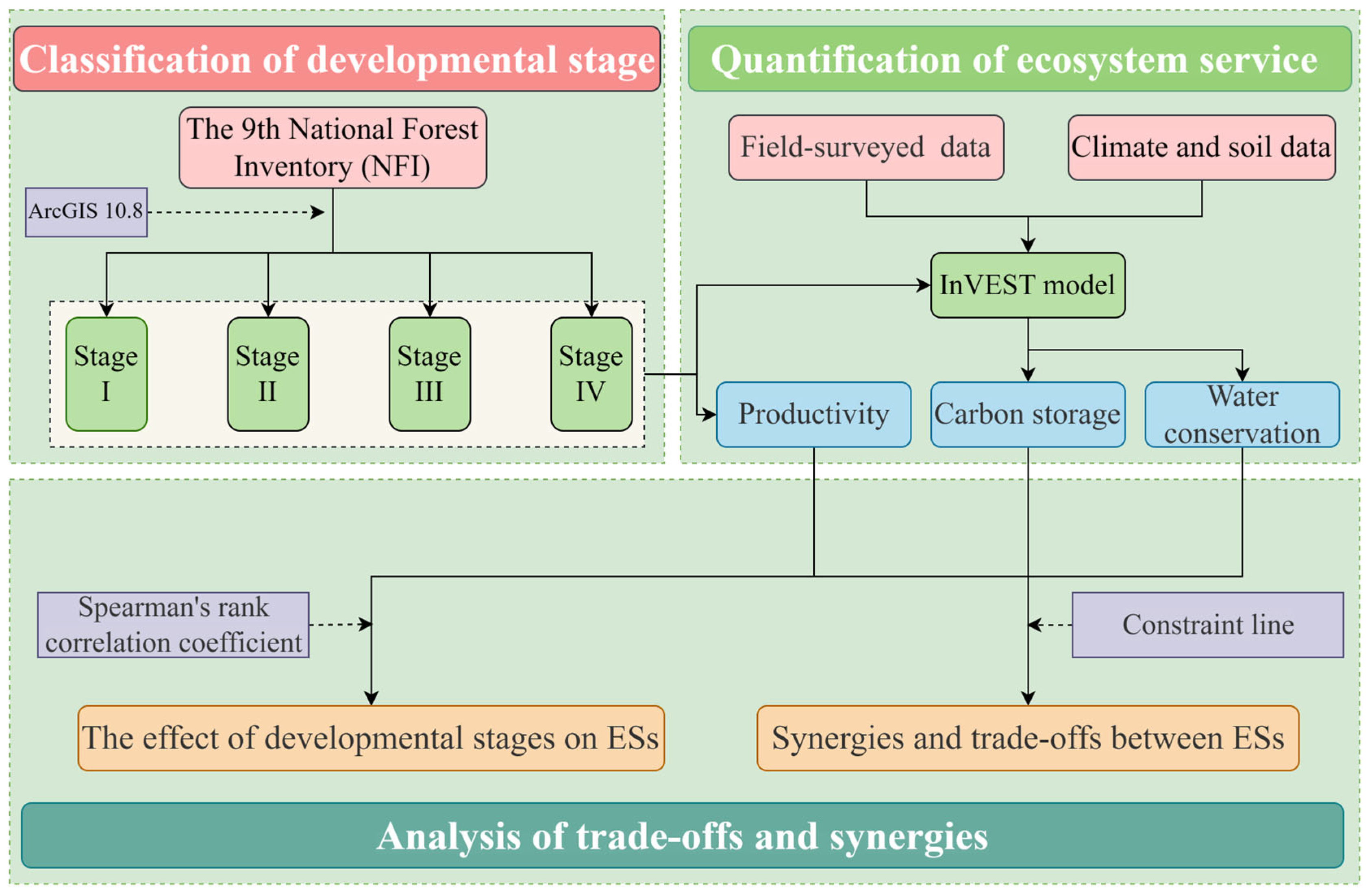
2. Materials and Methods

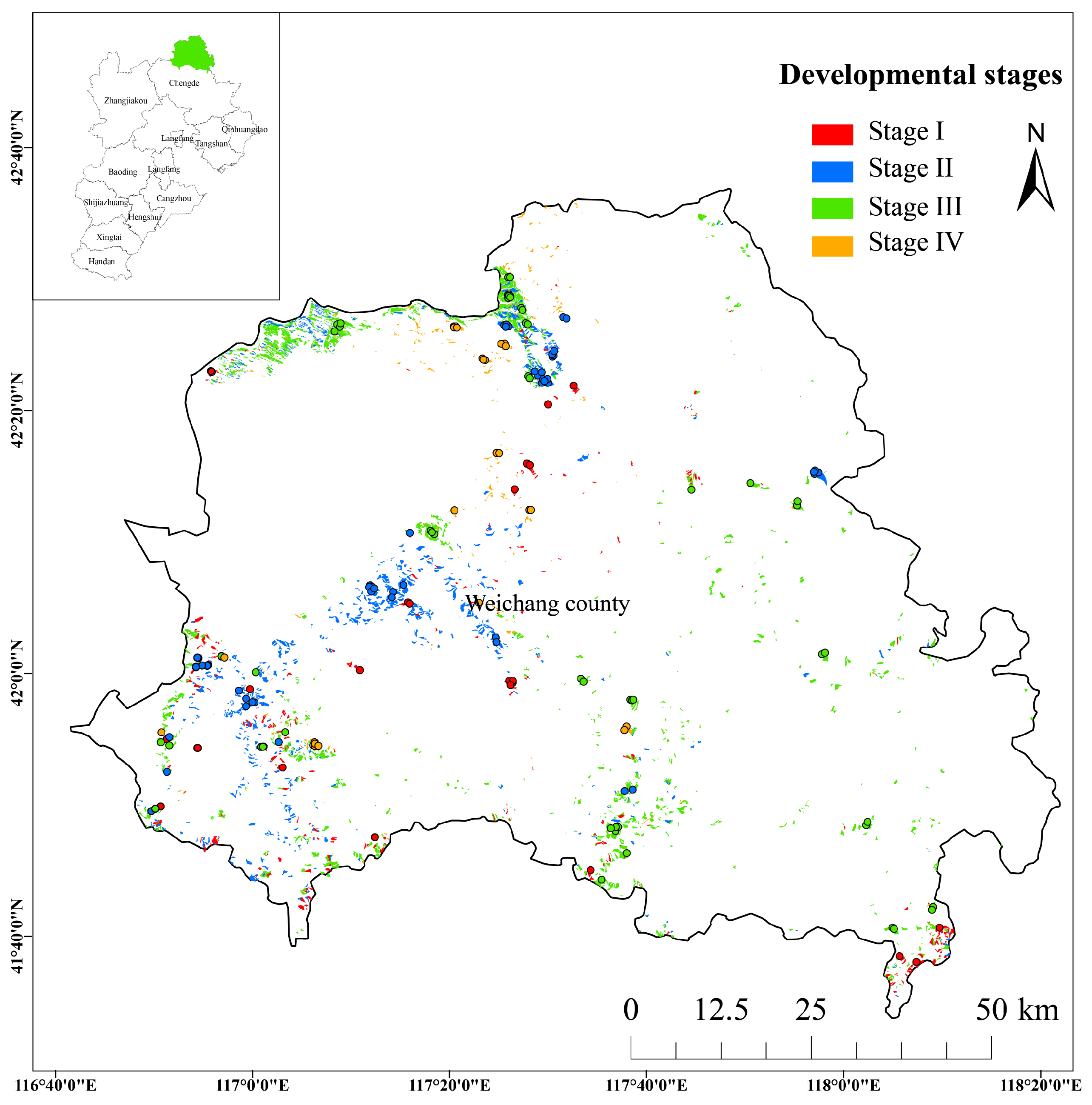
2.1. Study Area and Sample Plots

The study was conducted in Weichang County, Chengde City, Hebei Province, China (42°02′–42°36′ N, 116°51′–117°39′ E). It is located at the intersection of the North Hebei Mountains and the Mongolian Plateau, with elevations ranging from 750 to 1939.9 m. The region is characterized by a cold temperate continental monsoon climate, with an average annual temperature of about −1.3 °C, an extreme maximum temperature of 33.4 °C, and an extreme minimum temperature of −43.3 °C. The frost-free period varies between 67 and 128 days, and the average annual precipitation is between 380 and 560 mm. The area includes two Forest Farms: the Saihanba Mechanical Forest Farm and the Mulan Weichang State Forest Farm. Dominant tree species in the region include larch, birch, Mongolian pine (Pinus sylvestris var. mongolica), Mongolian oak, spruce, and poplar (Figure 1).

Developmental stages for MPB were classified based on the 2022 National Forest Inventory data. Based on species composition, the age of dominant species, and the proportion of climax species, MPB were categorized into four developmental stages. Stage I represented young natural secondary forests dominated by poplar and birch, with dominant species less than 30 years old and absent climax species. Stage II featured secondary forests with dominant species aged 30 to 50 years, in which climax species like spruce and larch were well-established. Stage III described a mixed forest of spruce, larch, poplar, and birch, marked by intense interspecific competition, a decreasing proportion of poplar and birch, and an increasing proportion of spruce and larch. Stage IV was characterized by secondary forests dominated by the climax species, larch, accompanied by birch, with dominant tree species over 60 years old.

To determine carbon density values across developmental stages of MPB, 148 sample plots were established from July to August 2022. The plots were distributed as follows: Stage I: 23 plots; Stage II: 49 plots; Stage III: 52 plots; Stage IV: 34 plots. Plot size was 50 m $\times$ 50 m (Figure 1). All trees with DBH > 5 cm were measured. The recorded factors included DBH, tree height, crown width, and relative coordinates (

Table 1. Basic information of sample plots.

Developmental Stage	Dominant Species	Basal Area (m2)	Mean Age (a)	Mean DBH (cm)	Mean Height (m)	Number of Plots
Stage I	Pd	5.06 (33.06)	28	10.7	11.3	23
	Bp	6.67 (43.59)		12.4	10.9
Stage II	Pd	9.19 (48.52)	35	11.5	12.6	49
	Bp	6.72 (45.33)		14.8	11.9
Stage III	Bp	6.01 (29.55)	51	15.7	13.8	52
	Lr	13.08 (64.39)		18.5	13.4
Stage IV	Lr	12.61 (54.69)	64	19.6	15.5	34

Pd is Populus davidiana, Bp is Betula platyphylla, Lr is Larix principis-rupprechtii. Brackets in the table indicate the percentage of the basal area of the dominant tree.

).

2.2. Data Sources and Processing

In this study, a multi-source dataset was collected for ES assessment and analysis (

Table A1. Description of the study data.

Data	Source	Resolution (m)	Pre-Processing Methods	Format
Climate data	The high-resolution climate model ClimateAP [70]	50	Firstly, bilinear interpolation and dynamic local regression were used to downscale monthly data from the ClimateAP model to scale-free point values. Then, the Barrier Spline Function Interpolation Tool in ArcGIS was used to create a rasterized climate dataset of the study area.	Raster
Topographic data	Geospatial Data Cloud (https://www.gscloud.cn) (accessed on 5 December 2023)	50	Using ArcGIS 10.8, the original projection was converted into WGS_1984_UTM_Zone_50N through the “Projection” tool. Subsequently, the corresponding data were extracted based on the vector of the study area by means of the “Extract by Mask” tool or the “Clip” tool.	Raster
Soil data	Mapping high resolution National Soil Information Grids of China [71]	90		Raster
Root restricting layer depth	Depth-to-bedrock map of China [72]	100		Raster
Watershed data	China metropolis group of basic geographic data (1951–2023) [73]	-		vector
Land Use/Land Cover data	Forest inventory data	50	Based on the screening principles, ArcGIS 10.8 was used to precisely extract the distribution information of different developmental stages of poplar (Populus davidiana)–birch (Betula platyphylla) mixed natural secondary forests (MPB) from the forest resource inventory data, and then the distribution ranges of MPB were determined.	Raster

). During the field survey, soil sampling was systematically conducted at five points along the diagonal of each sample plot, with two soil depths (0–10 cm and 10–20 cm) being sampled. The collected samples were then transported to the laboratory for further analysis. Following preparatory procedures, including soaking, weighing, and drying, the obtained soil indicators were used to calculate soil carbon density. The soil indicators included organic carbon content, total fresh weight, water content, and soil bulk density.

2.3. Calculating Ecosystem Services

2.3.1. Quantifying Carbon Storage

To estimate carbon density, a conversion factor relating biomass to carbon density was applied (Table 2). Dead litter samples were collected from the 158 sample plots. The physical properties and organic carbon densities of the soil samples were determined. The organic carbon densities of both dead organic matter and soil were derived using the corresponding models (Table 3).

The carbon storage (CS) and sequestration module of the InVEST model was employed to quantify and analyze the spatial distribution of CS in the study area. The InVEST model categorizes ecosystem CS into four main components: above-ground biomass carbon, below-ground biomass carbon, soil organic carbon, and dead organic matter carbon. Categorized land use data were used to calculate the average carbon density for each component of CS in MPB at various developmental stages. By determining the area occupied by each land use type, the total CS for the entire study area was calculated [25]. The model is outlined as follows [26]:

$$C_{\mathit{total}}=C_{\mathit{above}}+C_{\mathit{below}}+C_{\mathit{dead}}+C_{\mathit{soil}}$$

(1)

where C_total is total CS (t/ha), C_above is above-ground CS (t/ha), C_below is below-ground CS (t/ha), C_dead is dead organic CS (t/ha), and C_soil is soil CS (t/ha).

Raster data of land use types and carbon density parameters for each carbon pool were input into the CS module of the InVEST model in the ArcGIS 10.8 platform [27]. This process generated spatial distribution maps of CS in MPB at different developmental stages in the study area.

Table 2. Biomass models of tree species in the study area.

Tree Species	Biomass Model	Carbon Stock Conversion Factor	References
Betula platyphylla	W = $0.07367 \times$$D^{2.1085} \times$ H0.5202	0.487	[28]
Populus davidiana	W = $0.04703 \times$$D^{2.12487} \times$ H0.5916	0.471
Larix principis-rupprechtii	W = $0.06233 \times$$D^{2.01549} \times$ H0.5915	0.489
Picea asperata	W = $0.0807 \times$$D^{2.25957} \times$ H0.2566	0.490
Betula pendula	W = $0.07367 \times$$D^{2.1085} \times$ H0.5202	0.487
Tilia mongolica	W = $0.03798 \times$$D^{2.12825} \times$ H0.61117	0.475
Ulmus pumila	W = $0.10266 \times$$D^{1.9852} \times$ H0.4907	0.450
Pinus sylvestris var. mongolica	W = $0.0546 \times$$D^{2.23412} \times$ H0.3476	0.484
Quercus mongolica	W = $-1.3395+0.0555 \times$$D^2 \times$ H	0.500	[29]

“W” represents the aboveground biomass of the tree species (kg), “D” denotes the diameter at breast height (DBH) (cm), and “H” is the tree height (m).

Table 2. Biomass models of tree species in the study area.

Tree Species	Biomass Model	Carbon Stock Conversion Factor	References
Betula platyphylla	W = $0.07367 \times$$D^{2.1085} \times$ H0.5202	0.487	[28]
Populus davidiana	W = $0.04703 \times$$D^{2.12487} \times$ H0.5916	0.471
Larix principis-rupprechtii	W = $0.06233 \times$$D^{2.01549} \times$ H0.5915	0.489
Picea asperata	W = $0.0807 \times$$D^{2.25957} \times$ H0.2566	0.490
Betula pendula	W = $0.07367 \times$$D^{2.1085} \times$ H0.5202	0.487
Tilia mongolica	W = $0.03798 \times$$D^{2.12825} \times$ H0.61117	0.475
Ulmus pumila	W = $0.10266 \times$$D^{1.9852} \times$ H0.4907	0.450
Pinus sylvestris var. mongolica	W = $0.0546 \times$$D^{2.23412} \times$ H0.3476	0.484
Quercus mongolica	W = $-1.3395+0.0555 \times$$D^2 \times$ H	0.500	[29]

“W” represents the aboveground biomass of the tree species (kg), “D” denotes the diameter at breast height (DBH) (cm), and “H” is the tree height (m).

Table 3. Carbon density data acquisition.

Carbon Density	Formula	Interpretation	References
Belowground	$C_{below}=C_{above}\times b$	Cbelow is the below-ground carbon density (kg/km2); Cabove is the above-ground carbon density (kg/km2); and b is the ratio of below-ground biomass to above-ground biomass. The b value of forest land was set at 0.36 in this study.	[30]
Dead organic matter	$C_{dead}=TOC\times G\times W\times 10^{-5}$	Cdead is dead organic carbon density (kg/hm2); TOC is organic carbon content (g/kg); G is the total fresh weight of the sample in a 1 m × 1 m sample plot (g); W is the water content of the sample (%)	[31]
Soil organic matter	$C_{soil}=TOC\times y\times H\times 10^{-1}$	Csoil is soil organic carbon density (kg/hm2); TOC is organic carbon content(g/kg); y is soil density (g/cm3); H is average soil thickness (cm)	[32]

Table 3. Carbon density data acquisition.

Carbon Density	Formula	Interpretation	References
Belowground	$C_{below}=C_{above}\times b$	Cbelow is the below-ground carbon density (kg/km2); Cabove is the above-ground carbon density (kg/km2); and b is the ratio of below-ground biomass to above-ground biomass. The b value of forest land was set at 0.36 in this study.	[30]
Dead organic matter	$C_{dead}=TOC\times G\times W\times 10^{-5}$	Cdead is dead organic carbon density (kg/hm2); TOC is organic carbon content (g/kg); G is the total fresh weight of the sample in a 1 m × 1 m sample plot (g); W is the water content of the sample (%)	[31]
Soil organic matter	$C_{soil}=TOC\times y\times H\times 10^{-1}$	Csoil is soil organic carbon density (kg/hm2); TOC is organic carbon content(g/kg); y is soil density (g/cm3); H is average soil thickness (cm)	[32]

2.3.2. Quantify Productivity

In this study, annual mean biomass increment (BI) was identified as a metric for calculating forest productivity [33,34].

$$\mathit{BI}=(W_n-W_{n-T})/T$$

(2)

where W_n and W_n−T are the biomass in n and n − T years, respectively, and T is the study period.

2.3.3. Quantifying Water Conservation

The water conservation (WC) of MPB at different developmental stages was calculated for 2022 using the InVEST annual water yield module [5]. This model is based on the Budyko curve [35] and average annual precipitation. The annual water supply at different developmental stages of MPB was simulated using data on vegetation type, root limiting layer depth, effective water content of plants, land use cover, root depth, elevation, and water consumption. The formula used in the module is as follows:

$$Y_{\left(x\right)}=(1-{\displaystyle \frac{{\mathit{AET}}_{\left(x\right)}}{P_{\left(x\right)}}})\times P_{\left(x\right)}$$

(3)

where Y_(x) is the annual water production (mm) of raster image x, AET_(x) is the annual actual evapotranspiration (mm), and P_(x) is the annual precipitation (mm).

WC was obtained by correcting the water supply (WS) using the topographic index (T_x), saturated hydraulic conductivity of the soil (K_sat), and velocity coefficient (V_lx) [36]. The calculation is as follows:

$$\mathit{WC}=\min (1,{\displaystyle \frac{249}{V_{\mathit{lx}}}})\times \min (1,0.3\times T_x)\times \min (1,{\displaystyle \frac{K_{\mathit{sat},\mathit{x}}}{300}})\times Y_x$$

(4)

$$T_x=\lg ({\displaystyle \frac{A_{\mathit{drainage},x}}{d_{\mathit{soil},x}\times S_{\mathit{percent},x}}})$$

(5)

where WC is the water conservation (mm); V_lx is the flow coefficient of land use lx; T_x is the topographic index; K_sat,x is the saturated hydraulic conductivity of the soil (mm·d⁻¹); Y_x is the water yield (mm); A_drainage,x is the regional catchment runoff; d_soil,x is the soil thickness (mm); S_percent,x is the slope percentage.

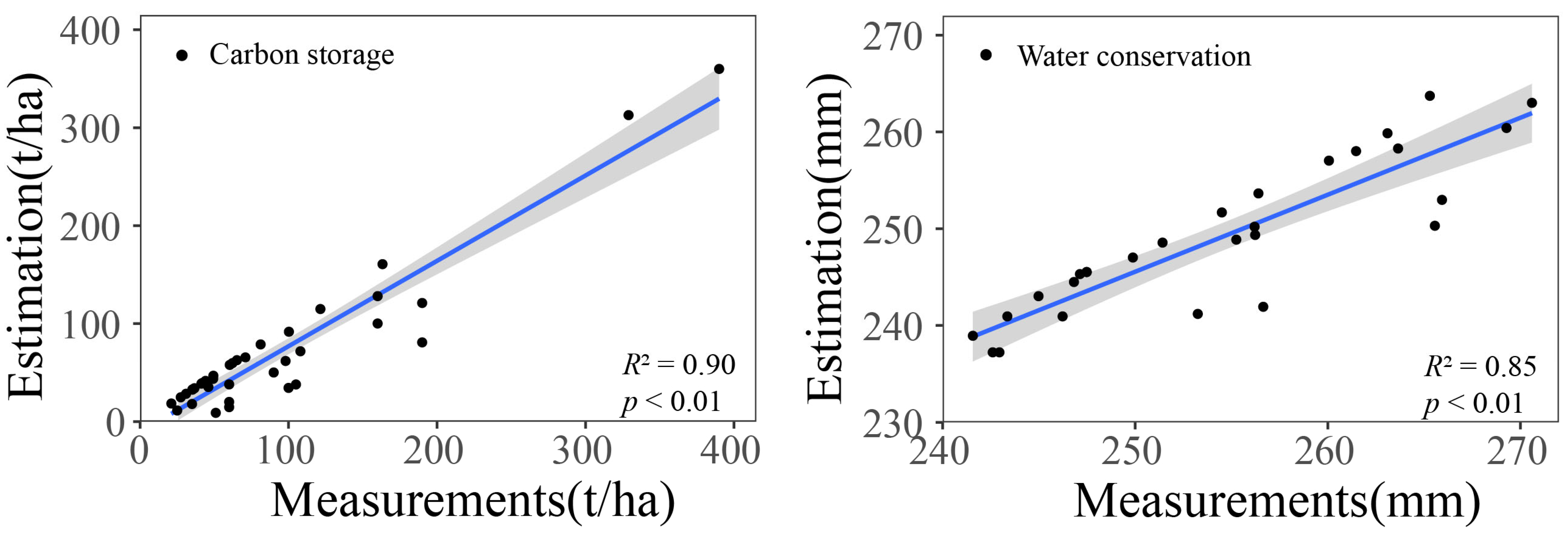
2.4. Validation for InVEST Model

Annual runoff data from hydrological stations and CS data obtained from field surveys were used to compare the output results of the InVEST model’s annual water yield (WY) and CS modules. The Pearson correlation coefficient [37] was used to assess the accuracy of the InVEST model (Figure 2).

The R² values for the fit of simulated to observed values for both the WY and CS models were greater than 0.80 (p < 0.01) (Figure 2), indicating that the models’ accuracies were acceptable.

2.5. Ecosystem Service Trade-Offs/Synergies

To analyze the impact of developmental stages on ESs, this study employed a one-way analysis of variance [38]. Spearman’s rank correlation coefficient was used to explore the relationships between CS, BI, and WC. The significance of these correlations was evaluated by a p-value test, with a threshold of p < 0.05 indicating substantial trade-offs or synergistic effects between services [39]. The constraint line method was employed to assess trade-offs and synergies among ESs. The DBSCAN clustering algorithm [21] was applied to detect outliers in the normalized dataset and to categorize data points into intervals. The maximum data point in each interval was then used to establish a constraint line through a polynomial function. The area-weighted average of each subclass was considered the representative value for the ES. Directional analysis of the constraint lines facilitated the inference of their shapes and the selection of the most analogous forms, including straight lines, convex curves, hump curves [40], and half-concave curves [21] (Figure 3).

CS and BI are supporting services provided by forest ecosystems, with WC serving as a key regulating service [41]. These supporting services are essential for improving the quality of mountain forests and preserving regional biodiversity. Recognizing their critical role in maintaining ecosystem balance and delivering long-term ecological benefits, this study prioritized CS and BI as key variables in evaluating their impact on WC. This strategic focus ensures that the significance of these fundamental services is fully considered in the assessment and management of ESs. Data processing was conducted using the R4.3.2 platform [42].

The analysis steps of this study are illustrated in Figure 4.

3. Results

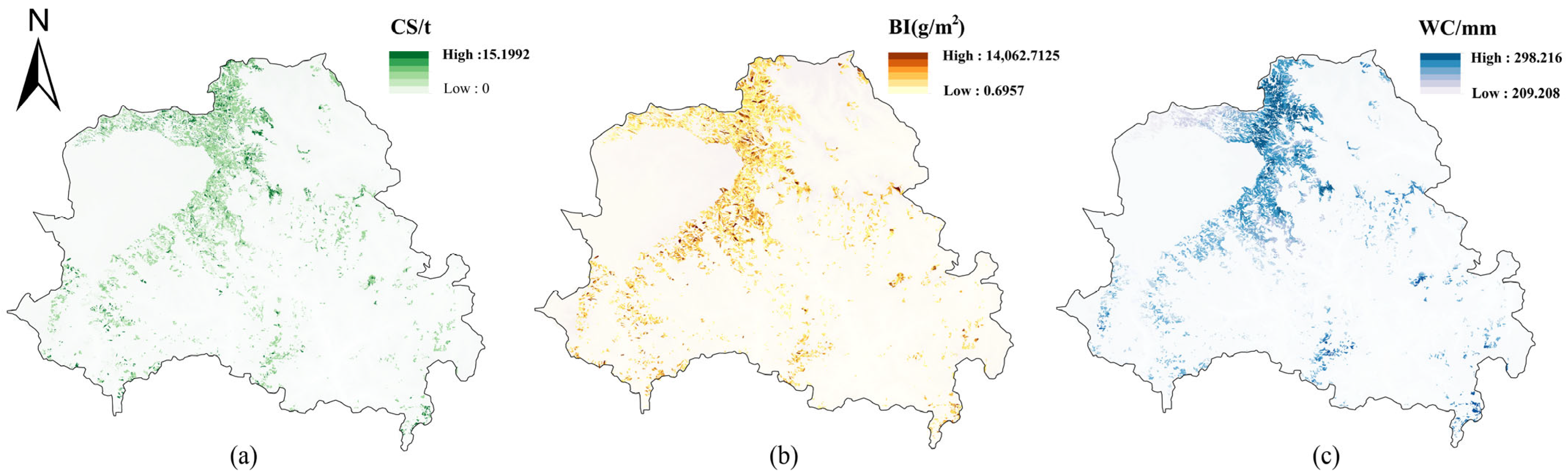
3.1. Spatial Distribution of Ecosystem Services

The spatial distribution patterns of the three ESs in the study area were similar, with high-value regions primarily located in the northwestern and central sections, and a more scattered distribution observed in the eastern region (Figure 5). Notably, the high CS area mostly overlaps with the high BI area in the northwest region. In contrast, only a small number of high WC patches coincided with areas of high CS and BI. The maximum values for CS, BI, and WC were 15.20 t/900 m², 14,062.71 g/m², and 298.22 mm, respectively. Among the three ESs, spatial heterogeneity was most significant for BI, followed by CS and WC.

3.2. Changes in Ecosystem Services with Developmental Stage

Differences in the distribution of the three ESs were observed across various developmental stages (Figure 6). As the stand development increased, CS values gradually increased, with significantly higher values recorded in the middle and late stages compared to the early stages (p < 0.05). BI remained relatively low during the initial three stages but exhibited a significant upward trend by Stage IV (p < 0.05). In contrast, WC did not exhibit a clear pattern of change with stand development.

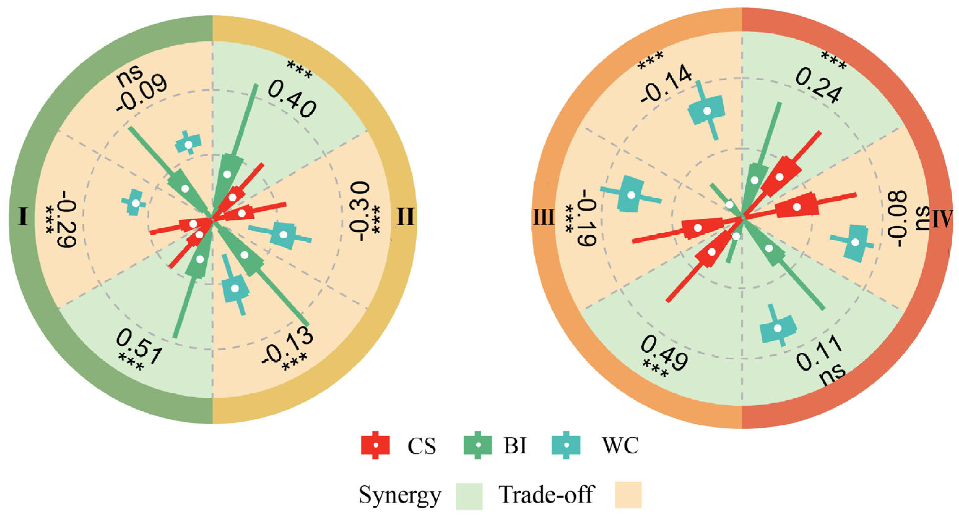
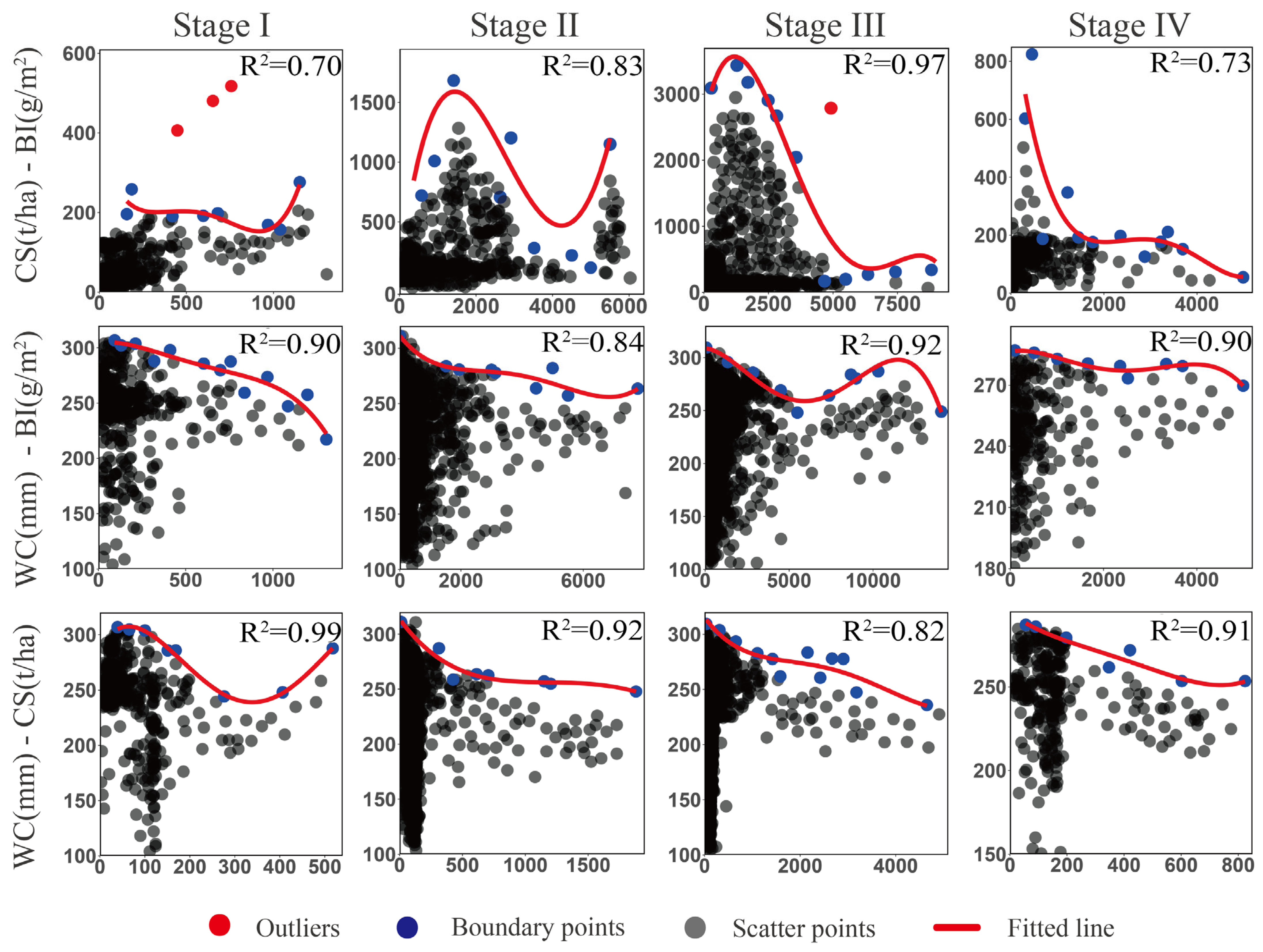
3.3. Trade-Offs/Synergies in Ecosystem Services

During the first three stages of stand development, a significant synergistic relationship was observed between BI and CS (Figure 7). However, this synergistic effect decreased in Stage IV. In the early stages, a strong trade-off relationship between WC and BI was present, which shifted to a weaker synergistic relationship in Stage IV. Similarly, the trade-off relationship between WC and CS weakened as the stand development increased.

The relationship between BI and CS exhibited an insignificant concave curve in Stage I, transitioning to a half-convex curve in Stage II and III, and evolving into a significant logarithmic trend in Stage IV. This pattern indicated that CS growth stabilized once BI exceeded a specific threshold (Figure 8). The relationship between BI and WC showed an insignificant negative linear trend in Stage I, II, and IV, while Stage III showed a concave curve, reflecting a fluctuating decline in WC with increasing BI. The relationship between CS and WC showed a half-convex trend in Stage I, while Stages II, III, and IV all exhibited a non-significant negative linear trend.

4. Discussion

4.1. Changes in Ecosystem Services with Developmental Stage

This study revealed that CS in the later stages of MPB was significantly higher than that in the earlier stages, indicating an increased carbon accumulation capacity as forests matured. This trend was likely driven by the complexity of the stand structure, enhanced biomass accumulation, and increased species diversity [43]. The enhanced carbon sequestration observed in later stages (III–IV) likely results from the dominance of climax species, such as spruce and larch, which exhibit higher wood density and slower litter decomposition rates [44]. Notably, no significant difference in CS was observed between Stage IV and Stage III, suggesting that CS stabilized in the late mature stage. This result was consistent with the findings of Molina-Valero et al. [45]. During MPB succession, the dominant tree species gradually shift from birch and poplar to larch. The stable canopy structure established by these dominant species optimizes light-use efficiency [46], while reduced interspecific competition following the decline of pioneer species facilitates resource allocation [47]. Upon entering Stage IV, productivity increased significantly, indicating higher resource utilization efficiency and more complex stand structures in mature forests, consistent with the findings of Pretzsch and Schütze [48]. Our finding emphasized the critical role of mature forests in biomass accumulation and CS optimization. However, WC capacity did not show a clear pattern across stand development stages, likely due to the multifactorial influences on this capacity [49]. Stand structure, soil properties, and vegetation cover collectively influenced the forest’s ability to intercept, infiltrate, and regulate evapotranspiration [50,51]. High transpiration rates in pioneer-dominated early stages may offset their superficial root water retention capacity [52], whereas improved soil infiltration from accumulated litter layers in later stages might be counteracted by diminished canopy interception [53]. The study emphasized the necessity of considering developmental stages in MPB management. Tailored management strategies are essential to improve ESs and forest resilience at different stages. For example, strategies aimed at optimizing CS should prioritize the protection and restoration of mature MPB. Meanwhile, management efforts focusing on biomass and WC should be adapted to the specific developmental stage. For example, thinning intensity should be progressively reduced from Stage I to Stage IV to align with the resource allocation patterns characteristic of forest succession. This gradual adjustment supports the transition from early-stage growth promotion to late-stage structural stability and ES enhancement.

4.2. Trade-Offs/Synergies Between BI and CS

The stable synergistic relationship between BI and CS in the initial three developmental stages of MPB indicated that productivity enhancement effectively complemented carbon sink capacity growth, consistent with Wang’s findings [54]. This relationship showed distinct dynamic patterns across succession phases: Stage I exhibited an insignificant concave curve, suggesting early secondary forest succession may experience temporary CS reduction due to high soil nutrient and water dependency [55]. As the ecosystem matured, biomass accumulation progressively enhanced CS capacity, transitioning to a half-convex curve in Stages II–III. This pattern reflected slowing CS growth rates despite continued biomass increases, correlating with stand structural changes including canopy closure, understory vegetation reduction, and soil organic matter equilibrium [56]. These dynamics held significant value for optimizing forest management and enhancing MPB’s carbon sequestration potential. However, Stage IV revealed a critical transition—the synergistic relationship weakened significantly and shifted to a logarithmic curve, indicating BI’s contribution to CS diminished beyond a threshold. This signaled potential ecosystem service saturation or ecological threshold attainment, where productivity increases no longer proportionally enhance CS [57]. The maturation processes of secondary forests likely drive this transition: biomass allocation shifts towards structural maintenance rather than CS enhancement [58], while complex stand structures promote internal carbon cycling processes like deadfall decomposition and soil organic matter dynamics [59]. Environmental factor variations in soil nutrients, precipitation, and temperature patterns may further constrain MPB’s carbon sequestration capacity during this stage. Notably, the logarithmic relationship in Stage IV suggests rapid recovery of soil carbon and nutrient cycling to primary forest levels [60], emphasizing the need for differentiated management strategies across developmental stages.

4.3. Trade-Offs/Synergies Between WC and BI

Our analysis revealed dynamic shifts in the WC and BI relationship across MPB developmental stages. During Stages I–III, a significant trade-off relationship emerged (Figure 8), where productivity gains negatively impacted WC capacity [61]. This inverse correlation was weakest among all ES pairs, suggesting additional mediating factors including soil properties, precipitation regimes, and vegetation composition may regulate these interactions [62]. The observed negative linear trend implies productivity-driven water constraints, likely due to elevated soil moisture demands during biomass accumulation. Stage III exhibited distinctive concave curvature, revealing non-monotonic WC responses to BI increases. This nonlinear pattern suggests mid-successional ecosystems develop compensatory mechanisms through biophysical adjustments—potentially via enhanced canopy precipitation interception coupled with increased transpiration [63], understory vegetation changes, and root system modifications [64]. Such complexity underscores the need for integrated management strategies incorporating structural adjustments and soil optimization during MPB’s intermediate phases. Notably, Stage IV demonstrated a paradigm shift from trade-off to weak synergy, indicating emerging equilibrium states in mature forest ecosystems [65]. While statistically unstable, this reversal highlights maturation-stage ecological thresholds where long-term processes may reconcile ES conflicts. The transition carries critical implications for global change adaptation, emphasizing mature forest preservation to maintain emergent synergies. The observed synergy supports a rationale for prohibiting clear-cutting in mature MPB forests. Instead, the implementation of low-intensity selection cutting during drought years is recommended to sustain the balance between WC and BI.

4.4. Trade-Offs/Synergies Between WC and CS

Our analysis revealed stage-dependent interactions between CS and WC during MPB succession. In Stage I, ecosystem recovery prioritized biomass accumulation through rapid carbon sequestration, coinciding with reduced water retention capacity [66]. This trade-off manifested as a non-linear concave relationship, potentially driven by three interconnected processes: early vegetation recovery patterns, organic matter accumulation altering soil hydrology, and transitional root system development [58]. As secondary succession progressed to intermediate and late stages (Stages II–III), the CS/WC trade-off intensity diminished significantly, paralleling increases in ecosystem structural complexity. Mature stands demonstrated enhanced multifunctionality through: vertically stratified canopy architecture, biodiversity-driven niche differentiation, and improved soil hydrological regulation [67]. These developments enabled concurrent optimization of both carbon storage and water conservation capacities. However, late-successional stands exhibited renewed competition between CS and WC, characterized by canopy closure reducing precipitation infiltration, increased transpirational water demand from biomass accumulation, and rhizosphere competition intensifying soil moisture heterogeneity [68,69]. This phenomenon suggests that maintaining water-holding capacity should be considered in forest management alongside efforts to increase CS, to ensure a balanced provision of ESs and the long-term sustainability of forests. Future research should further explore the interactions between these processes to support the development of effective forest management strategies.

4.5. Limitations and Future Directions

While this study provided valuable insights into ESs, several limitations should be acknowledged. First, the analysis focused on CS, WC, and BI, while omitting key indicators such as biodiversity, soil stability, and cultural services. This limited the ability to fully assess the multifaceted impacts of forest management. Second, although synergies and trade-offs among ESs were identified, management interventions—such as varying thinning intensities or implementing mixed-species planting—were not experimentally validated, constraining practical recommendations for optimizing ES provision. Third, the influence of developmental stages on forest resilience to climate stressors (e.g., droughts) was not evaluated, thereby limiting insights into adaptive strategies under climate change. Future research should address these limitations by: (1) incorporating additional indicators, including biodiversity metrics, soil stability indices, and cultural services, to support a more comprehensive assessment of forest management outcomes; (2) conducting controlled experiments to evaluate adaptive strategies—such as thinning regimes and species mixing—for enhancing synergistic ES provision; and (3) examining how different developmental stages modulate forest responses to climate extremes in order to inform climate-resilient management practices.

5. Conclusions

This study assessed the synergies and trade-offs between ESs in MPB across various successional stages. The results revealed that BI and CS increased throughout MPB succession, whereas WC exhibited no consistent pattern across stages. A significant synergy between BI and CS was observed in the earlier stages of MPB succession, though this relationship weakened in later stages due to shifts in carbon allocation, offering a novel mechanistic explanation that challenges the assumption of persistent synergy in mature forests. Initially, a trade-off existed between WC and BI. However, this shifted to a synergistic relationship as succession progressed, providing the first empirical evidence of hydrological self-regulation in temperate mixed forests. Similarly, the trade-off between WC and CS diminished over time. The innovative application of constraint line analysis revealed dynamic trade-offs among BI, CS, and WC, indicating potential saturation in ES provision and the existence of ecological thresholds in MPB forests. These insights support a stage-adaptive management framework: mature MPB forests should be prioritized for protection to maximize synergies between CS and WC, while early-stage stands may benefit from targeted interventions—such as selective thinning and understory retention—to accelerate ES recovery. By incorporating dynamic ES thresholds into management strategies, this study offers a new paradigm for successional forest management under changing environmental conditions.

References

1. Guo, Z.L.; Liu, Y.N.; Zhang, L.; Feng, C.Y.; Chen, Y.M. Research progress and prospect of ecosystem services. J. Environ. Eng. Technol. 2022, 12, 928–936. [Google Scholar] [CrossRef]
2. Nunes, L.J.R.; Meireles, C.I.R.; Pinto Gomes, C.J.; Almeida Ribeiro, N.M.C. Forest contribution to climate change mitigation: Management oriented to carbon capture and storage. Climate 2020, 8, 21. [Google Scholar] [CrossRef]
3. Jin, J.; Xiang, W.H.; Zeng, Y.L.; Ouyang, S.; Zhou, X.L.; Hu, Y.T.; Zhao, Z.H.; Chen, L.; Lei, P.F.; Deng, X.W.; et al. Stand carbon storage and net primary production in China’s subtropical secondary forests are predicted to increase by 2060. Carbon Balance Manag. 2022, 17, 6–14. [Google Scholar] [CrossRef]
4. Biber, P.; Felton, A.; Nieuwenhuis, M.; Lindbladh, M.; Black, K.; Bahýl, J.; Bingöl, Ö.; Borges, J.G.; Botequim, B.; Brukas, V.; et al. Forest biodiversity, carbon sequestration, and wood production: Modeling synergies and trade-offs for ten forest landscapes across Europe. Front. Ecol. Evol. 2020, 8, 547696. [Google Scholar] [CrossRef]
5. Yan, X.; Cao, G.C.; Cao, S.K.; Yuan, J.; Zhao, M.L.; Tong, S.; Li, H.D. Spatiotemporal variations of water conservation and its influencing factors in the Qinghai Plateau, China. Ecol. Indic. 2023, 155, 111047. [Google Scholar] [CrossRef]
6. Sandifer, P.A.; Sutton-Grier, A.E.; Ward, B.P. Exploring connections among nature, biodiversity, ecosystem services, and human health and well-being: Opportunities to enhance health and biodiversity conservation. Ecosyst. Serv. 2015, 12, 1–15. [Google Scholar] [CrossRef]
7. Darvishi, A.; Yousefi, M.; Dinan, N.M.; Angelstam, P. Assessing levels, trade-offs and synergies of landscape services in the Iranian province of Qazvin: Towards sustainable landscapes. Landscape Ecol. 2022, 37, 305–327. [Google Scholar] [CrossRef]
8. Mazziotta, A.; Lundström, J.; Forsell, N.; Moor, H.; Eggers, J.; Subramanian, N.; Aquilué, N.; Morán-Ordóñez, A.; Brotons, L.; Snäll, T. More future synergies and less trade-offs between forest ecosystem services with natural climate solutions instead of bioeconomy solutions. Glob. Change Biol. 2022, 28, 6333–6348. [Google Scholar] [CrossRef]
9. Gutsch, M.; Lasch-Born, P.; Kollas, C.; Suckow, F.; Reyer, C.P. Balancing trade-offs between ecosystem services in Germany’s forests under climate change. Environ. Res. Lett. 2018, 13, 045012. [Google Scholar] [CrossRef]
10. Soimakallio, S.; Kalliokoski, T.; Lehtonen, A.; Salminen, O. On the trade-offs and synergies between forest carbon sequestration and substitution. Mitig. Adapt. Strat. Gl. 2021, 26, 4. [Google Scholar] [CrossRef]
11. Morán-Ordóñez, A.; Ameztegui, A.; De Cáceres, M.; de-Miguel, S.; Lefèvre, F.; Brotons, L.; Coll, L. Future trade-offs and synergies among ecosystem services in Mediterranean forests under global change scenarios. Ecosyst. Serv. 2020, 45, 101174. [Google Scholar] [CrossRef]
12. Agol, D.; Reid, H.; Crick, F.; Wendo, H. Ecosystem-based adaptation in Lake Victoria Basin; synergies and trade-offs. R. Soc. Open Sci. 2021, 8, 201847. [Google Scholar] [CrossRef]
13. Liu, H.; Zheng, L.; Wu, J.; Liao, Y.H. Past and future ecosystem service trade-offs in Poyang Lake basin under different land use policy scenarios. Arab. J. Geosci. 2020, 13, 46. [Google Scholar] [CrossRef]
14. Karimi, J.D.; Corstanje, R.; Harris, J.A. Bundling ecosystem services at a high resolution in the UK: Trade-offs and synergies in urban landscapes. Landscape Ecol. 2021, 36, 1817–1835. [Google Scholar] [CrossRef]
15. Yang, Q.Q.; Zhang, P.; Qiu, X.C.; Xu, G.L.; Chi, J.Y. Spatial-temporal variations and trade-offs of ecosystem services in Anhui Province, China. Int. J. Env. Res. Public Health 2023, 20, 855. [Google Scholar] [CrossRef] [PubMed]
16. Meraj, G.; Singh, S.K.; Kanga, S.; Islam, M.N. Modeling on comparison of ecosystem services concepts, tools, methods and their ecological—Economic implications: A review. Model. Earth Syst. Environ. 2022, 8, 15–34. [Google Scholar] [CrossRef]
17. Zou, K.H.; Tuncali, K.; Silverman, S.G. Correlation and simple linear regression. Radiology 2003, 227, 617–628. [Google Scholar] [CrossRef] [PubMed]
18. Andrew, M.E.; Wulder, M.A.; Nelson, T.A.; Coops, N.C. Spatial data, analysis approaches, and information needs for spatial ecosystem service assessments: A review. GISci. Remote Sens. 2015, 52, 344–373. [Google Scholar] [CrossRef]
19. Knoke, T.; Kindu, M.; Jarisch, I.; Gosling, E.; Friedrich, S.; Bödeker, K.; Paul, C. How considering multiple criteria, uncertainty scenarios and biological interactions may influence the optimal silvicultural strategy for a mixed forest. For. Policy Econ. 2020, 118, 102239. [Google Scholar] [CrossRef]
20. Zuo, L.Y.; Gao, J.B.; Du, F.J. The pairwise interaction of environmental factors for ecosystem services relationships in karst ecological priority protection and key restoration areas. Ecol. Indic. 2021, 131, 108125. [Google Scholar] [CrossRef]
21. Ding, X.M.; Jian, S.Q. Synergies and trade-offs of ecosystem services affected by land use structures of small watershed in the Loess Plateau. J. Environ. Manag. 2024, 350, 119589. [Google Scholar] [CrossRef] [PubMed]
22. Hao, R.F.; Yu, D.Y.; Wu, J.G. Relationship between paired ecosystem services in the grassland and agro—Pastoral transitional zone of China using the constraint line method. Agric. Ecosyst. Environ. 2017, 240, 171–181. [Google Scholar] [CrossRef]
23. Zhang, J.; Liu, C.; Ge, Z.X.; Zhang, Z.D. Stand spatial structure and productivity based on random structural unit in Larix principis-rupprechtii forests. Ecosphere 2024, 15, e4824. [Google Scholar] [CrossRef]
24. Bohnett, E.; An, L. Special issue editorial: Biodiversity and ecosystem services in forest ecosystems. Sustainability 2023, 15, 16364. [Google Scholar] [CrossRef]
25. Costanza, R.; de Groot, R.; Sutton, P.; van der Ploeg, S.; Anderson, S.J.; Kubiszewski, I.; Farber, S.; Turner, R.K. Changes in the global value of ecosystem services. Global Environ. Change 2014, 26, 152–158. [Google Scholar] [CrossRef]
26. Clerici, N.; Cote-Navarro, F.; Escobedo, F.J.; Rubiano, K.; Villegas, J.C. Spatio—Temporal and cumulative effects of land use—Land cover and climate change on two ecosystem services in the Colombian Andes. Sci. Total Environ. 2019, 685, 1181–1192. [Google Scholar] [CrossRef]
27. Esri. ArcGIS Desktop: Release 10.8. Redlands, CA: Environmental Systems Research Institute. 2020. Available online: https://desktop.arcgis.com/ (accessed on 10 December 2023).
28. GB/T 43648-2024; Tree Biomass Models and Related Parameters to Carbon Accounting for Major Tree Species. Standards Press of China: Beijing, China, 2024.
29. Sun, H.L. Estimation of biomass in Mongolian oak forests of the northern Hebei Mountain region. Shandong For. Sci. Technol. 2018, 48, 44–45. [Google Scholar]
30. Rajashekar, G.; Fararoda, R.; Reddy, R.S.; Jha, C.S.; Ganeshaiah, K.N.; Singh, J.S.; Dadhwal, V.K. Spatial distribution of forest biomass carbon (above and below ground) in Indian forests. Ecol. Indic. 2018, 85, 742–752. [Google Scholar] [CrossRef]
31. Lin, Y.C.; Zhang, J.M.; Zhou, Y.N.; Guan, Y.H.; Zhou, J.X. Analyzing spatial distribution of carbon storage and hot spots in Xiaoluan river basin in Weichang County based on InVEST model. Chin. J. Ecol. 2023, 42, 2536. [Google Scholar]
32. Rong, Y.J.; Zhang, H.; Zhao, X.F. Carbon stock functions under land use change in the Lake Tai basin in the last 10 years based on InVEST modeling. Jiangsu Agric. Sci. 2016, 5, 447–451. [Google Scholar]
33. Djomo, A.N.; Knohl, A.; Gravenhorst, G. Estimations of total ecosystem carbon pools distribution and carbon biomass current annual increment of a moist tropical forest. For. Ecol. Manag. 2011, 261, 1448–1459. [Google Scholar] [CrossRef]
34. He, X.; Lei, X.D.; Dong, L.H. How large is the difference in large-scale forest biomass estimations based on new climate-modified stand biomass models? Ecol. Indic. 2021, 126, 107569. [Google Scholar] [CrossRef]
35. Zhang, L.; Hickel, K.; Dawes, W.R.; Chiew, F.H.; Western, A.W.; Briggs, P.R. A rational function approach for estimating mean annual evapotranspiration. Water Resour. Res. 2004, 40, W02502. [Google Scholar] [CrossRef]
36. Yang, D.; Liu, W.; Tang, L.Y.; Chen, L.; Li, X.Z.; Xu, X.L. Estimation of water provision service for monsoon catchments of South China: Applicability of the InVEST model. Landscape Urban Plan. 2019, 182, 133–143. [Google Scholar] [CrossRef]
37. Sun, W.; Shao, Q.; Liu, J.; Zhai, J. Assessing the effects of land use and topography on soil erosion on the Loess Plateau in China. Catena 2014, 121, 151–163. [Google Scholar] [CrossRef]
38. Maxwell, S.E.; Delaney, H.D.; Kelley, K. Designing Experiments and Analyzing Data: A Model Comparison Perspective, 3rd ed.; Routledge: New York, NY, USA, 2017; p. 1080. [Google Scholar] [CrossRef]
39. Wang, S.M.; Jin, T.T.; Yan, L.L.; Gong, J. Trade—Off and synergy among ecosystem services and the influencing factors in the Ziwuling Region, Northwest China. Chin. J. Appl. Ecol. 2022, 33, 3087–3096. [Google Scholar] [CrossRef]
40. Hao, R.; Yu, D.; Wu, J.; Guo, Q.; Liu, Y. Constraint line methods and the applications in ecology. Chin. J. Plant Ecol. 2016, 40, 1100–1109. [Google Scholar] [CrossRef]
41. Millennium Ecosystem Assessment. Ecosystems and Human Well-Being: Synthesis; Island Press: Washington, DC, USA, 2005. [Google Scholar]
42. R Core Team. R Foundation for Statistical Computing, Vienna, Austria. 2023. Available online: https://www.r-project.org/ (accessed on 18 December 2023).
43. Hardiman, B.S.; Gough, C.M.; Halperin, A.; Hofmeister, K.L.; Nave, L.E.; Bohrer, G.; Curtis, P.S. Maintaining high rates of carbon storage in old forests: A mechanism linking canopy structure to forest function. For. Ecol. Manag. 2013, 298, 111–119. [Google Scholar] [CrossRef]
44. Prescott, C.E. Litter decomposition: What controls it and how can we alter it to sequester more carbon in forest soils? Biogeochem. 2010, 101, 133–149. [Google Scholar] [CrossRef]
45. Molina-Valero, J.A.; Camarero, J.J.; Álvarez-González, J.G.; Cerioni, M.; Hevia, A.; Sánchez-Salguero, R.; Martin-Benito, D.; Pérez-Cruzado, C. Mature forests hold maximum live biomass stocks. For. Ecol. Manag. 2021, 480, 118635. [Google Scholar] [CrossRef]
46. Forrester, D.I.; Bauhus, J. A review of processes behind diversity—Productivity relationships in forests. Curr. For. Rep. 2016, 2, 45–61. [Google Scholar] [CrossRef]
47. Kunstler, G.; Falster, D.; Coomes, D.A.; Hui, F.; Kooyman, R.M.; Laughlin, D.C.; Poorter, L.; Vanderwel, M.; Vieilledent, G.; Wright, S.G. Plant functional traits have globally consistent effects on competition. Nature 2016, 529, 204–207. [Google Scholar] [CrossRef]
48. Pretzsch, H.; Schütze, G. Tree species mixing can increase stand productivity, density and growth efficiency and attenuate the trade-off between density and growth throughout the whole rotation. Ann. Bot. 2021, 128, 767–786. [Google Scholar] [CrossRef] [PubMed]
49. Schwärzel, K.; Zhang, L.; Montanarella, L.; Wang, Y.; Sun, G. How afforestation affects the water cycle in drylands: A process-based comparative analysis. Glob. Change Biol. 2020, 26, 944–959. [Google Scholar] [CrossRef] [PubMed]
50. van Meerveld, H.J.; Jones, J.P.; Ghimire, C.P.; Zwartendijk, B.W.; Lahitiana, J.; Ravelona, M.; Mulligan, M. Forest regeneration can positively contribute to local hydrological ecosystem services: Implications for forest landscape restoration. J. Appl. Ecol. 2021, 58, 755–765. [Google Scholar] [CrossRef]
51. Ellison, D.; Morris, C.E.; Locatelli, B.; Sheil, D.; Cohen, J.; Murdiyarso, D.; Gutierrez, V.; Van Noordwijk, M.; Creed, I.F.; Pokorny, J. Trees, forests and water: Cool insights for a hot world. Glob. Environ. Change 2017, 43, 51–61. [Google Scholar] [CrossRef]
52. Sayer, E.J. Using experimental manipulation to assess the roles of leaf litter in the functioning of forest ecosystems. Biol. Rev. 2006, 81, 1–31. [Google Scholar] [CrossRef]
53. Xu, L.; Liu, Y.; Feng, S.; Liu, C.; Zhong, X.; Ren, Y.; Liu, Y.; Huang, Y.; Yang, M. The relationship between atmospheric particulate matter, leaf surface microstructure, and the phyllosphere microbial diversity of Ulmus L. BMC Plant Biol. 2024, 24, 566. [Google Scholar] [CrossRef]
54. Wang, X.Z.; Wu, J.Z.; Liu, Y.L.; Hai, X.Y.; Shanguan, Z.P.; Deng, L. Driving factors of ecosystem services and their spatiotemporal change assessment based on land use types in the Loess Plateau. J. Environ. Manag. 2022, 311, 114835. [Google Scholar] [CrossRef]
55. Teixeira, H.M.; Cardoso, I.M.; Bianchi, F.J.J.A.; da Cruz Silva, A.; Jamme, D.; Peña-Claros, M. Linking vegetation and soil functions during secondary forest succession in the Atlantic forest. For. Ecol. Manag. 2020, 457, 117696. [Google Scholar] [CrossRef]
56. Qiang, W.; He, L.L.; Zhang, Y.; Liu, B.; Liu, Y.; Liu, Q.H.; Pang, X.Y. Aboveground vegetation and soil physicochemical properties jointly drive the shift of soil microbial community during subalpine secondary succession in southwest China. Catena 2021, 202, 105251. [Google Scholar] [CrossRef]
57. Başkent, E.Z.; Kašpar, J. Exploring the effects of management intensification on multiple ecosystem services in an ecosystem management context. For. Ecol. Manag. 2022, 518, 120299. [Google Scholar] [CrossRef]
58. Harel, A.; Thiffault, E.; Paré, D. Ageing forests and carbon storage: A case study in boreal balsam fir stands. Forestry 2021, 94, 651–663. [Google Scholar] [CrossRef]
59. Prescott, C.E.; Vesterdal, L. Decomposition and transformations along the continuum from litter to soil organic matter in forest soils. For. Ecol. Manag. 2021, 498, 119522. [Google Scholar] [CrossRef]
60. Berry, Z.C.; Jones, K.W.; Aguilar, L.R.G.; Congalton, R.G.; Holwerda, F.; Kolka, R.; Looker, N.; Lopez Ramirez, S.M.; Manson, R.; Mayer, A.; et al. Evaluating ecosystem service trade-offs along a land—Use intensification gradient in central Veracruz, Mexico. Ecosyst. Serv. 2020, 45, 101181. [Google Scholar] [CrossRef]
61. Farooqi, T.J.A.; Li, X.H.; Yu, Z.; Liu, S.R.; Sun, O.J. Reconciliation of research on forest carbon sequestration and water conservation. J. For. Res. 2021, 32, 7–14. [Google Scholar] [CrossRef]
62. Pan, T.; Zuo, L.; Zhang, Z.; Zhao, X.; Sun, F.; Zhu, Z.; Liu, Y. Impact of land use change on water conservation: A case study of Zhangjiakou in Yongding River. Sustainability 2020, 13, 22. [Google Scholar] [CrossRef]
63. Ghimire, C.P.; Bruijnzeel, L.A.; Lubczynski, M.W.; Ravelona, M.; Zwartendijk, B.W.; van Meerveld, H.J. Measurement and modeling of rainfall interception by two differently aged secondary forests in upland eastern Madagascar. J. Hydrol. 2017, 545, 212–225. [Google Scholar] [CrossRef]
64. Hu, Y.T.; Zhang, F.; Luo, Z.Z.; Badreldin, N.; Benoy, G.; Xing, Z.S. Soil and water conservation effects of different types of vegetation cover on runoff and erosion driven by climate and underlying surface conditions. Catena 2023, 231, 107347. [Google Scholar] [CrossRef]
65. Souza, C.R.; Maia, V.A.; de Aguiar-Campos, N.; Santos, A.B.; Rodrigues, A.F.; Farrapo, C.L.; Gianasi, F.M.; de Paula, G.G.P.; Fagundes, N.C.A.; Silva, W.B.; et al. Long-term ecological trends of small secondary forests of the Atlantic forest hotspot: A 30-year study case. For. Ecol. Manag. 2021, 489, 119043. [Google Scholar] [CrossRef]
66. Asbjornsen, H.; Wang, Y.; Ellison, D.; Ashcraft, C.M.; Atallah, S.S.; Jones, K.; Mayer, A.; Altamirano, M.; Yu, P. Multi-targeted payments for the balanced management of hydrological and other forest ecosystem services. For. Ecol. Manag. 2022, 522, 120482. [Google Scholar] [CrossRef]
67. Liu, D.; Zhou, C.F.; He, X.; Zhang, X.H.; Feng, L.Y.; Zhang, H.R. The effect of stand density, biodiversity, and spatial structure on stand basal area increment in natural spruce-fir-broadleaf mixed forests. Forests 2022, 13, 162. [Google Scholar] [CrossRef]
68. Kurzweil, J.R.; Metlen, K.; Abdi, R.; Strahan, R.; Hogue, T.S. Surface water runoff response to forest management: Low-intensity forest restoration does not increase surface water yields. For. Ecol. Manag. 2021, 496, 119387. [Google Scholar] [CrossRef]
69. Gavrilescu, M. Water, soil, and plants interactions in a threatened environment. Water 2021, 13, 2746. [Google Scholar] [CrossRef]
70. Wang, T.; Wang, G.; Innes, J.L.; Seely, B.; Chen, B. ClimateAP: An application for dynamic local downscaling of historical and future climate data in Asia Pacific. Front. Agric. Sci. Eng. 2017, 4, 448–458. [Google Scholar] [CrossRef]
71. Liu, F.; Wu, H.Y.; Zhao, Y.G.; Li, D.C.; Yang, J.L.; Song, X.D.; Shi, Z.; Zhu, A.-X.; Zhang, G.L. Mapping high resolution National Soil Information Grids of China. Sci. Bull. 2021, 67, 328–340. [Google Scholar] [CrossRef]
72. Yan, F.; Shangguan, W.; Zhang, J.; Hu, B. Depth-to-bedrock map of China at a spatial resolution of 100 meters. Sci. Data 2020, 7, 2. [Google Scholar] [CrossRef]
73. China Metropolis Group of Basic Geographic Data (1951–2023). National Tibetan Plateau/Third Pole Environment Data Center. Available online: https://data.tpdc.ac.cn (accessed on 19 April 2023).
Figure 1. Distribution of poplar (Populus davidiana)–birch (Betula platyphylla) mixed natural secondary forests and sample plots at different developmental stages in the study area; the black circles are marked as the sample plots.
Forests 16 00867 g001
Figure 2. Verification for annual water yield (WY) model and carbon storage (CS) model.
Forests 16 00867 g002
Figure 3. Types of constraint lines: (a) positive linear line; (b) negative linear line; (c) negative curve; (d) exponential curve; (e) logarithmic curve; (f) S-shaped curve; (g) convex-waved curve; (h) concave-waved curve; (i) half-concave-waved curve; (j) half-convex waved curves.
Forests 16 00867 g003
Figure 4. The analysis steps for identifying trade-offs and synergies between ecosystem services.
Forests 16 00867 g004
Figure 5. Spatial distribution of ecosystem services in the study area. (a) carbon storage; (b) productivity; (c) water conservation.
Forests 16 00867 g005
Figure 6. Distribution and multiple comparison of ecosystem services across four developmental stages. Different letters indicate significant differences among developmental stages based on Tukey’s HSD test.
Forests 16 00867 g006
Figure 7. Trade-offs and synergies between ecosystem services in four developmental stages of poplar-birch mixed natural secondary forests. ***—p < 0.001, ns—p > 0.05.
Forests 16 00867 g007
Figure 8. Constraints between carbon storage, productivity, and water conservation in poplar–birch mixed natural secondary forests at four developmental stages. y-axis represents the paired ESs A–B, where A is the service on the y-axis of the scatterplot, and B corresponds to the service on the x-axis of the scatterplot.
Forests 16 00867 g008