
Deciphering Spatiotemporal Dynamics of Vegetation Drought Resilience in China

Abstract
1. Introduction
2. Materials and Methods
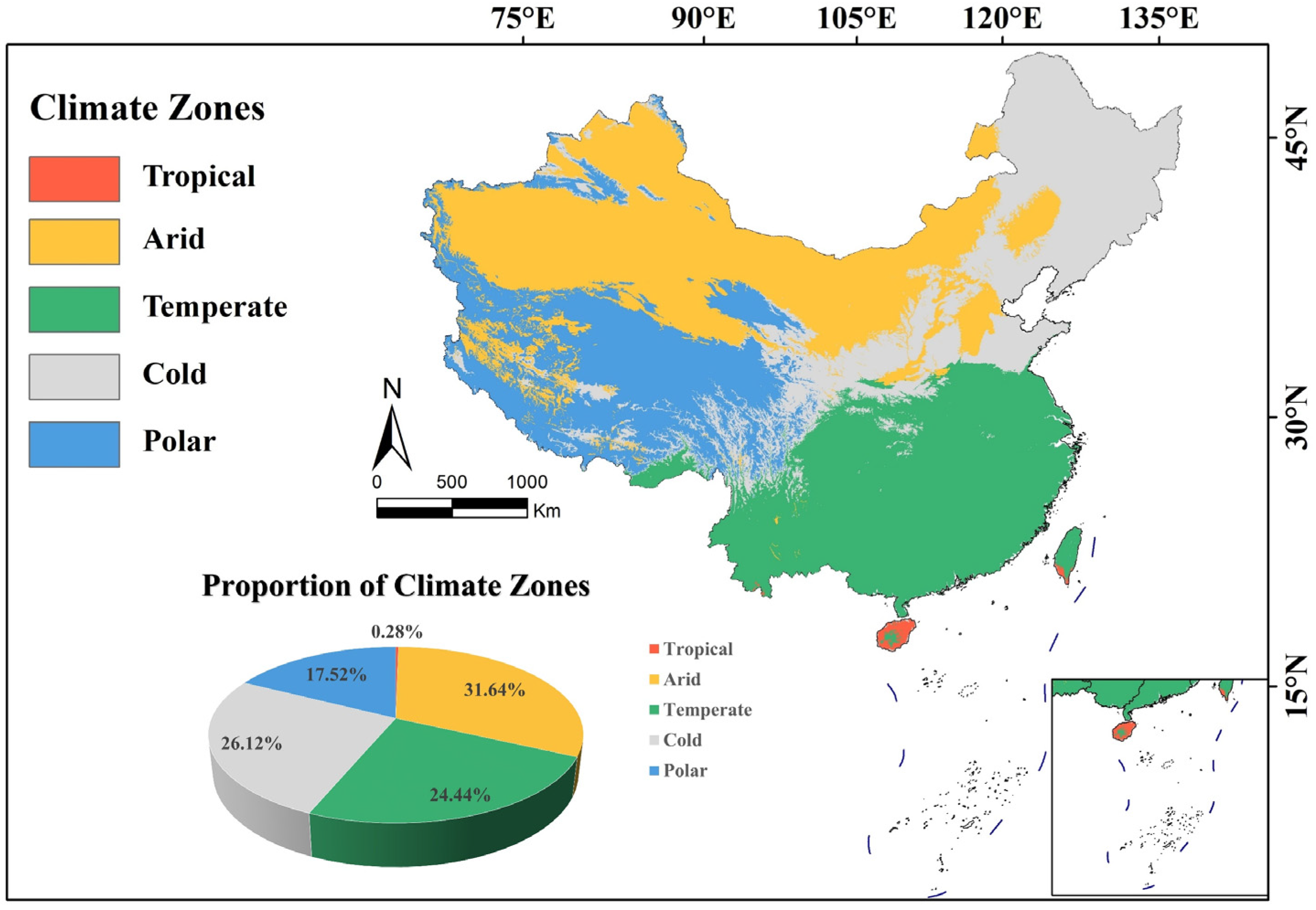
2.1. Study Area
2.2. Data Sources
2.2.1. Resilience Assessment Datasets
2.2.2. Driving Factor Datasets

| Dataset | Units | Description | Resolution | Source |
|---|---|---|---|---|
| PRE | 0.1 mm | Precipitation | 1 km monthly | [57] |
| TEM | °C | Temperature | 1 km monthly | [58] |
| GDP | USD | Gross Domestic Product | 1 km yearly | [61] |
| ODIAC | Pg | Anthropogenic Carbon Dioxide Emissions | 1 km yearly | [62] |
| PET | mm | Potential Evapotranspiration | 1 km monthly | [59] |
| SMCI | 10−3 m3/m3 | Soil Moisture Content Index | 1 km daily | [63] |
| VPD | hPa | Vapor Pressure Deficit | 1 km monthly | [64] |
| RH | % | Relative Humidity | 1 km monthly | |
| WIN | m/s | Wind Speed | 1 km yearly | [65] |
| SUN | h | Sunlight Hours | 1 km yearly |
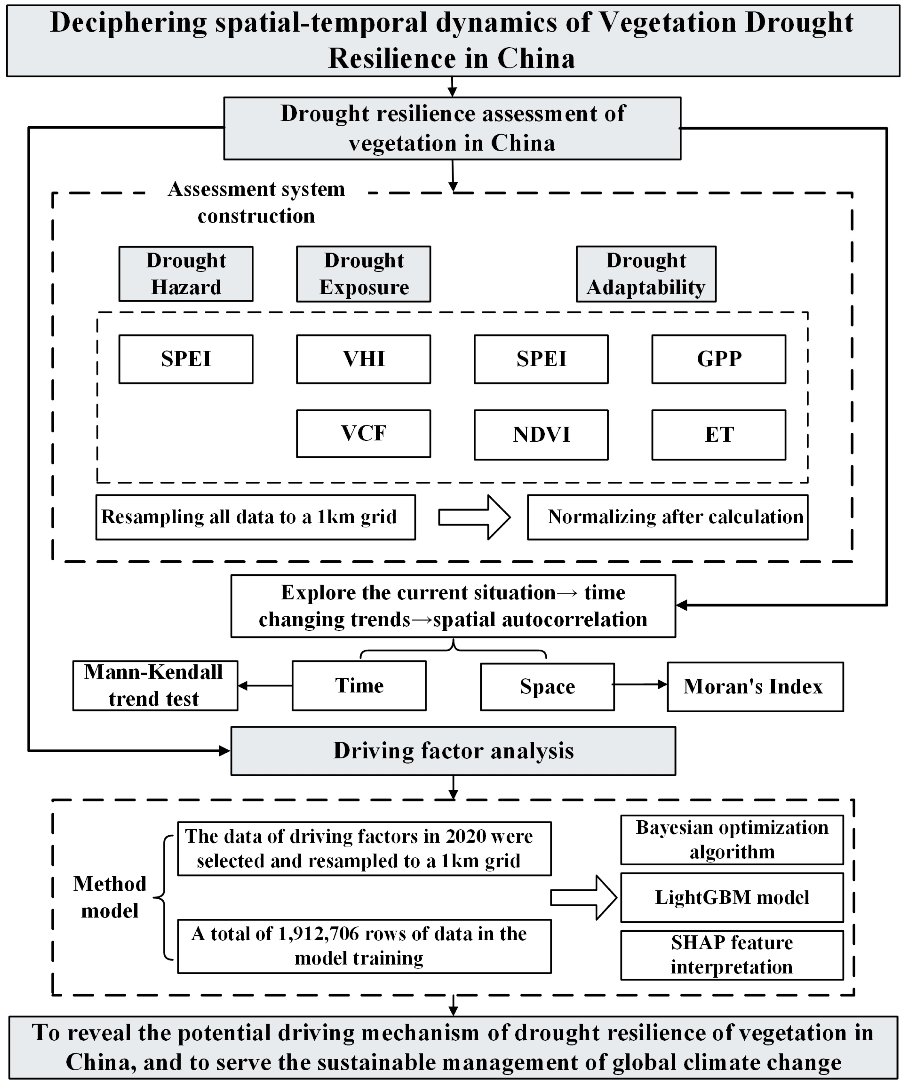
2.3. Methods
2.3.1. Assessment of DR
2.3.2. Analysis of DR Spatiotemporal Patterns
2.3.3. Analysis of DR Driving Factors
3. Results
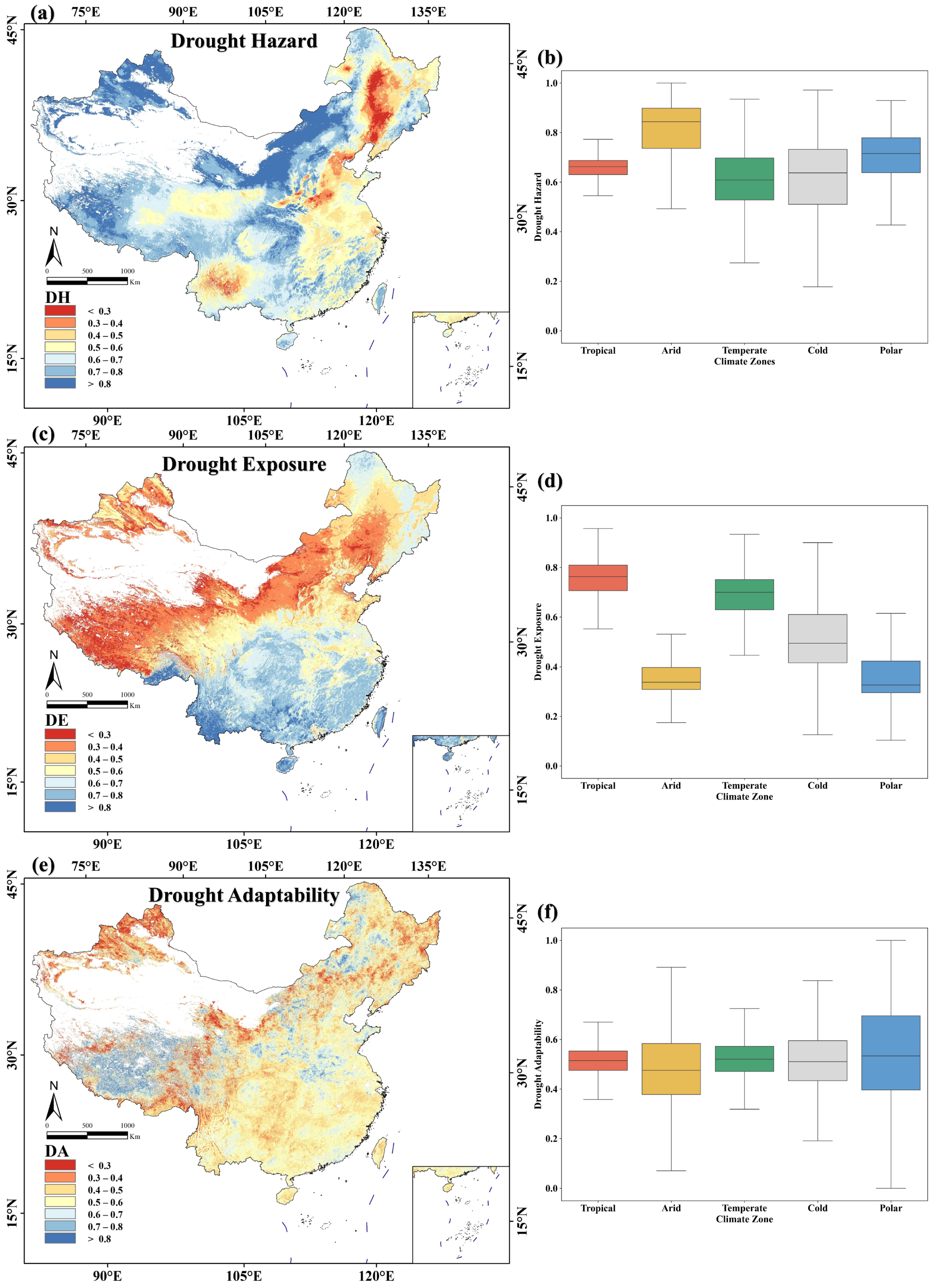
3.1. Patterns of DR Independent Components
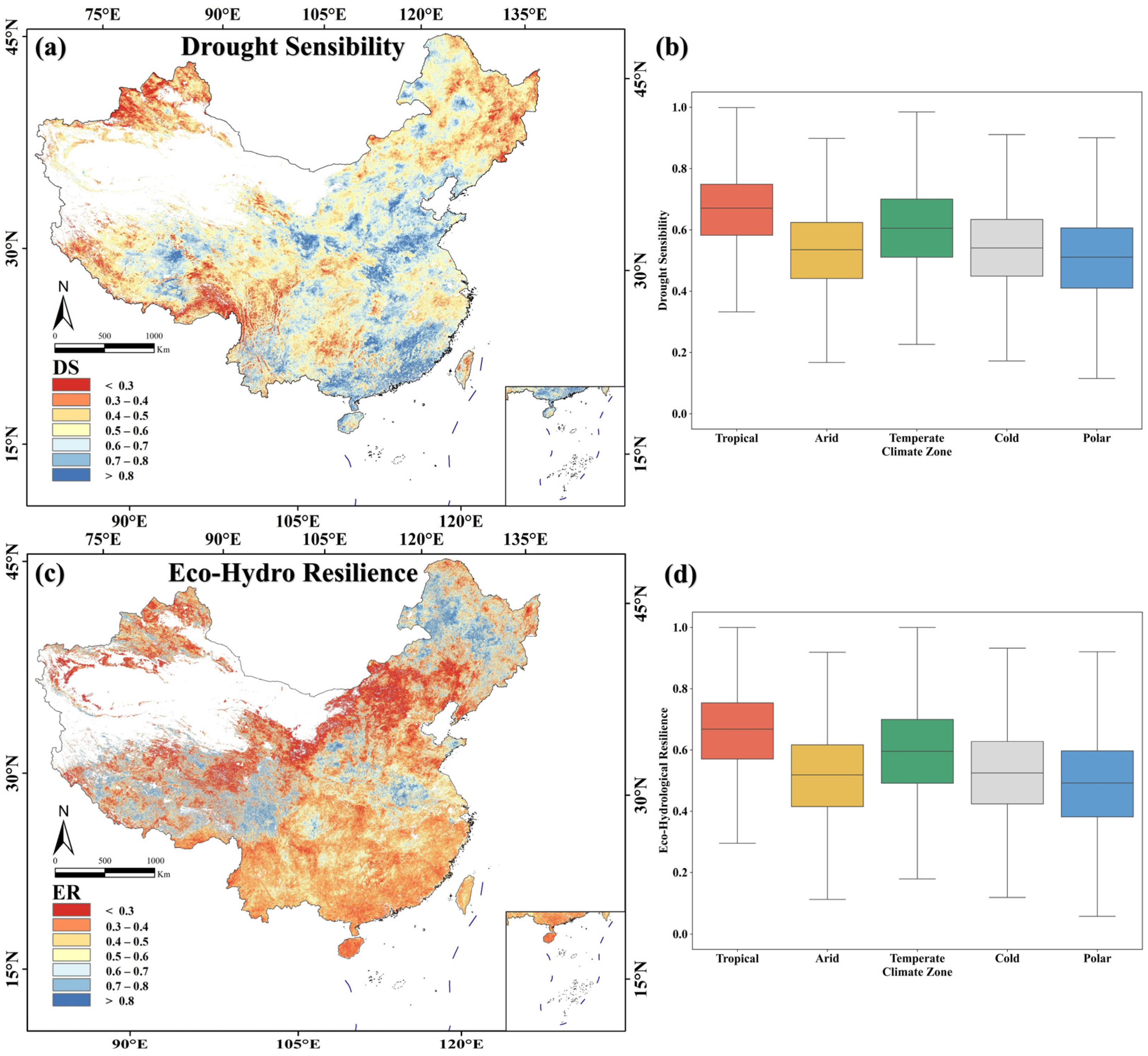
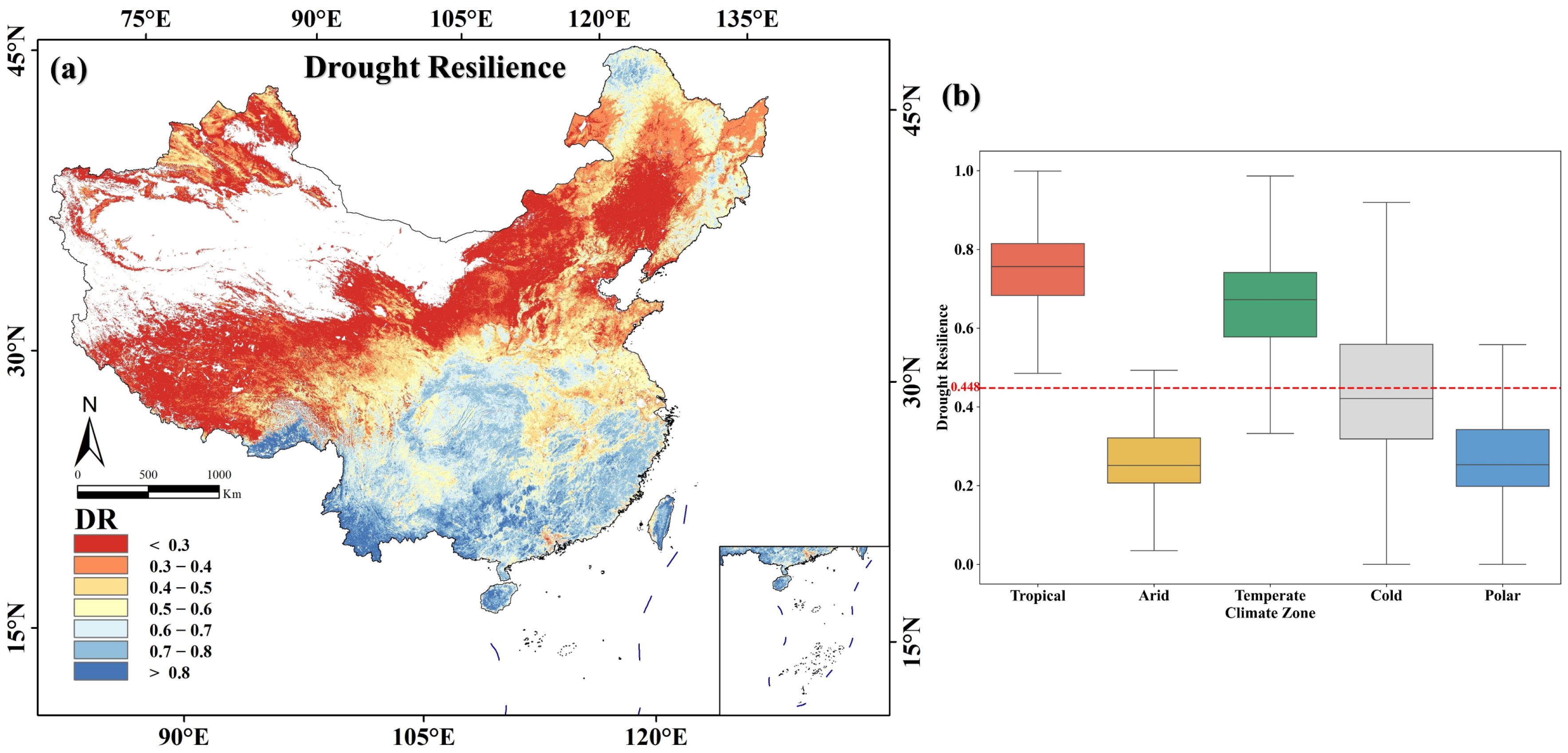
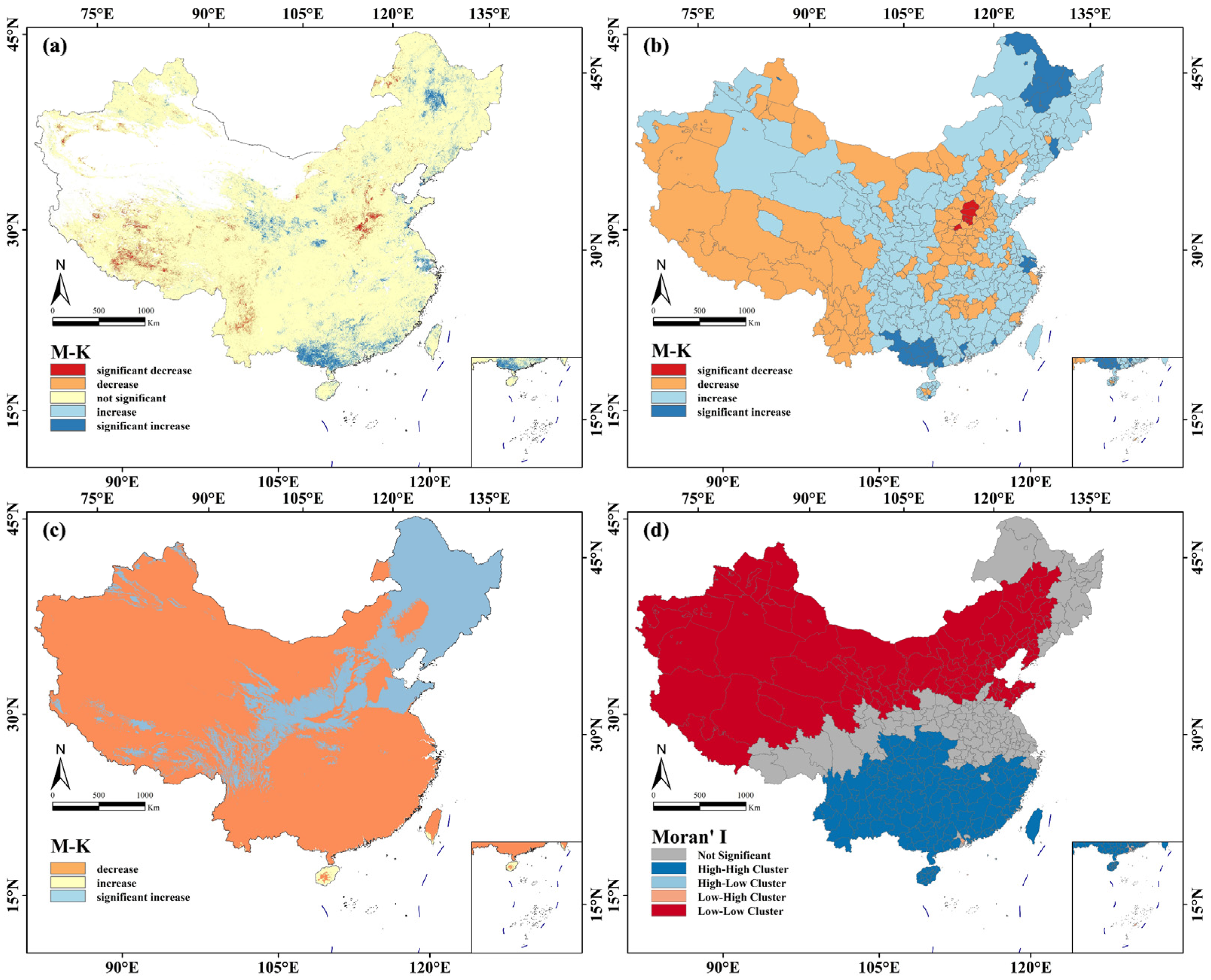
3.2. Spatiotemporal Patterns of DR
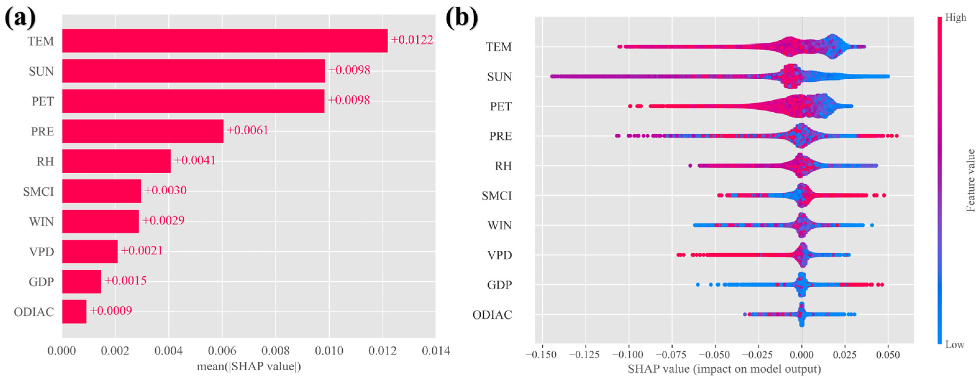
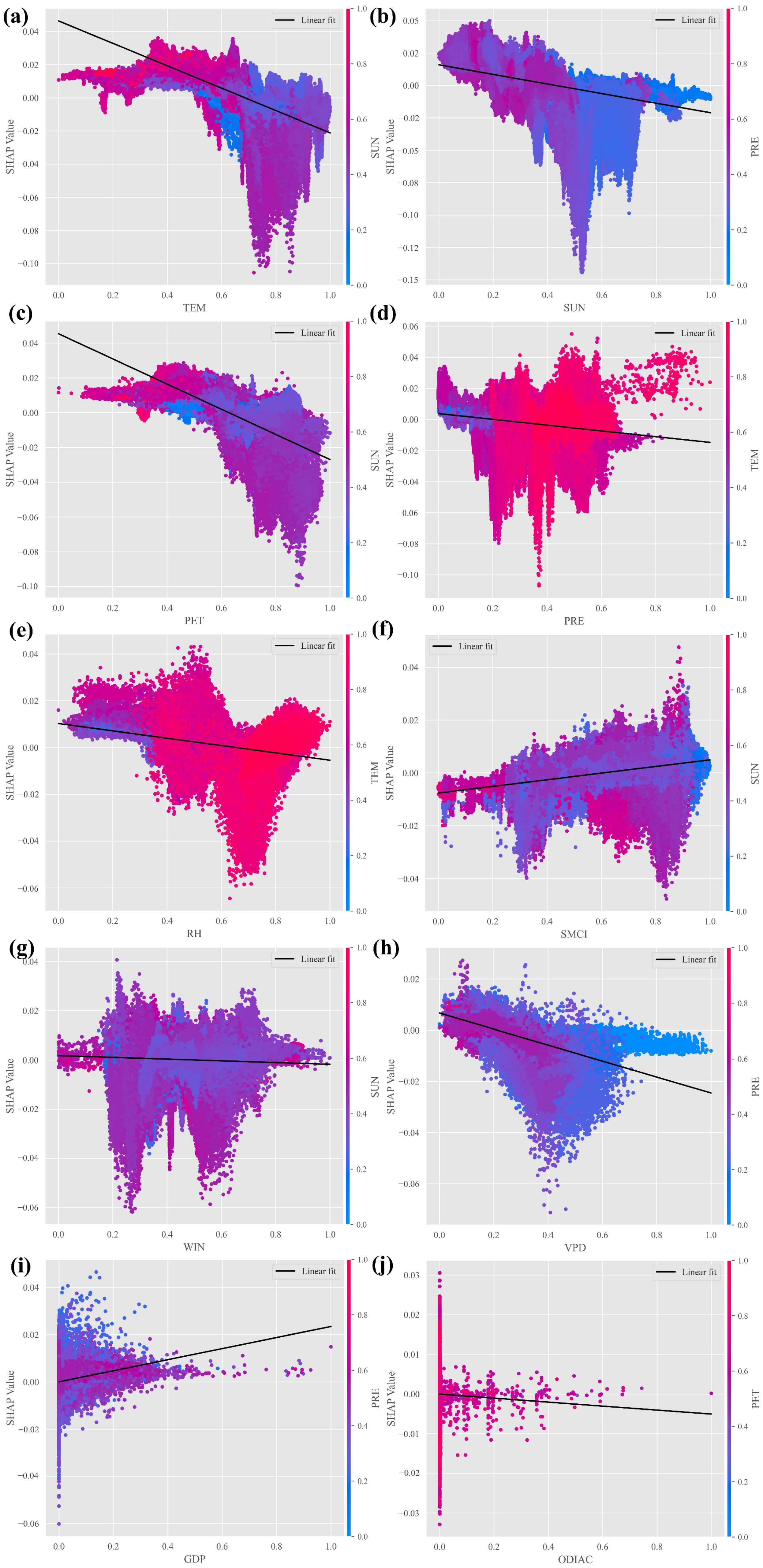
3.3. Modeling and Analysis of Driving Factors
4. Discussion
4.1. Drivers’ Interaction on DR
4.2. Spatial Differentiation and Regional Drivers of DR
4.3. Limitations
5. Conclusions
Supplementary Materials
Author Contributions
Funding
Data Availability Statement
Acknowledgments
Conflicts of Interest
Abbreviations
| DR | Drought Resilience |
| LightGBM | Light Gradient Boosting Machine |
| SHAP | Shapley Additive exPlanations |
| SPEI | Standardized Precipitation Evapotranspiration Index |
| LAI | Leaf Area Index |
| GPP | Gross Primary Productivity |
| WUE | Water Use Efficiency |
| SPI | Standardized Precipitation Index |
| PDSI | Palmer Drought Severity Index |
| HSPEI | High-resolution Standardized Precipitation Evapotranspiration Index |
| NDVI | Normalized Difference Vegetation Index |
| VCF | Vegetation Continuous Fields |
| ET | Evapotranspiration |
| LST | Land Surface Temperature |
| PRE | Precipitation |
| TEM | Temperature |
| GDP | Gross Domestic Product |
| ODIAC | Anthropogenic Carbon Dioxide Emissions |
| PET | Potential Evapotranspiration |
| SMCI | Soil Moisture Content Index |
| VPD | Vapor Pressure Deficit |
| RH | Relative Humidity |
| WIN | Wind Speed |
| SUN | Sunlight Hours |
| DH | Drought Hazard |
| DE | Drought Exposure |
| DA | Drought Adaptability |
| VHI | Health Condition of Vegetation |
| VD | Vegetation Density |
| VCI | Vegetation Condition Index |
| TCI | Temperature Condition Index |
| DS | Drought Sensitivity |
| ER | Eco-hydrological Resilience |
| RMSE | Root Mean Square Error |
| MSE | Mean Square Error |
| MAE | Mean Absolute Error |
References
- Chen, L.; Brun, P.; Buri, P.; Fatichi, S.; Gessler, A.; McCarthy, M.J.; Pellicciotti, F.; Stocker, B.; Karger, D.N. Global increase in the occurrence and impact of multiyear droughts. Science 2025, 387, 278–284. [Google Scholar] [CrossRef] [PubMed]
- Yuan, X.; Wang, Y.; Ji, P.; Wu, P.; Sheffield, J.; Otkin, J.A. A global transition to flash droughts under climate change. Science 2023, 380, 187–191. [Google Scholar] [CrossRef]
- Abhishek; Kinouchi, T. Multidecadal land water and groundwater drought evaluation in Peninsular India. Remote Sens. 2022, 14, 1486. [Google Scholar] [CrossRef]
- Williams, E.L.; Abatzoglou, J.T.; Hegewisch, K.C.; Williams, A.P. Anthropogenic climate change has reduced drought recovery probabilities across the western US. Commun. Earth Environ. 2024, 5, 546. [Google Scholar] [CrossRef]
- Huang, S.; Wang, S.; Chen, J.; Wang, C.; Zhang, X.; Wu, J.; Li, C.; Gulakhmadov, A.; Niyogi, D.; Chen, N. Urbanization-induced spatial and temporal patterns of local drought revealed by high-resolution fused remotely sensed datasets. Remote Sens. Environ. 2024, 313, 114378. [Google Scholar] [CrossRef]
- Huang, S.; Siqi, W.; Gan, Y.; Wang, C.; Horton, D.; Li, C.; Xiang, Z.; Niyogi, D.; Xia, J.; Chen, N. Widespread global exacerbation of extreme drought induced by urbanization. Nat. Cities 2024, 1, 597–609. [Google Scholar] [CrossRef]
- Zhang, Q.; Yao, Y.; Li, Y.; Huang, J.; Ma, Z.; Wang, Z.; Wang, S.; Wang, Y.; Zhang, Y. Progress and prospect on the study of causes and variation regularity of droughts in China (Chinese Edition). Acta Meteorol. Sin. 2020, 78, 500–521. [Google Scholar] [CrossRef]
- Compilation group of China Flood and Drought Disaster Prevention Bulletin. Summary of China Flood and Drought Disaster Prevention Bulletin 2022. China Flood Drought Manag. 2023, 33, 78–82. [Google Scholar] [CrossRef]
- Forootan, E.; Khaki, M.; Schumacher, M.; Wulfmeyer, V.; Mehrnegar, N.; van Dijk, A.I.; Brocca, L.; Farzaneh, S.; Akinluyi, F.; Ramillien, G. Understanding the global hydrological droughts of 2003–2016 and their relationships with teleconnections. Sci. Total Environ. 2019, 650, 2587–2604. [Google Scholar] [CrossRef]
- Oliveira, R.S.; Eller, C.B.; Barros, F.d.V.; Hirota, M.; Brum, M.; Bittencourt, P. Linking plant hydraulics and the fast–slow continuum to understand resilience to drought in tropical ecosystems. New Phytol. 2021, 230, 904–923. [Google Scholar] [CrossRef]
- Cao, H.H.; Chen, F.; Hu, M.; Hou, T.Y.; Zhao, X.E.; Wang, S.J.; Zhang, H.L. Tree-Ring Insights into Past and Future Streamflow Variations in Beijing, Northern China. Water Resour. Res. 2025, 61, e2024WR038084. [Google Scholar] [CrossRef]
- Yue, W.P.; Chen, F.; Torbenson, M.C.A.; Zhao, X.E.; Zheng, Y.H.; Xu, Y.; Hu, M.; Wang, S.J.; Hou, T.Y.; Zhang, H.L.; et al. Late Ming Dynasty weak monsoon induced a harmonized megadrought across north-to-south China. Commun. Earth Environ. 2024, 5, 439. [Google Scholar] [CrossRef]
- Chen, F.; Wang, S.J.; Dong, Q.J.; Esper, J.; Büntgen, U.; Meko, D.; Linderholm, H.W.; Wang, T.; Yue, W.P.; Zhao, X.E.; et al. Role of Pacific Ocean climate in regulating runoff in the source areas of water transfer projects on the Pacific Rim. npj Clim. Atmos. Sci. 2024, 7, 153. [Google Scholar] [CrossRef]
- Wu, X.F.; Tang, W.H.; Chen, F.; Wang, S.J.; Bakhtiyorov, Z.; Liu, Y.X.; Guan, Y.S. Attribution and Risk Projections of Hydrological Drought Over Water-Scarce Central Asia. Earth Future 2025, 13, e2024EF005243. [Google Scholar] [CrossRef]
- Li, J.; Zhang, Y.; Bevacqua, E.; Zscheischler, J.; Keenan, T.F.; Lian, X.; Zhou, S.; Zhang, H.Y.; He, M.Z.; Piao, S.L. Future increase in compound soil drought-heat extremes exacerbated by vegetation greening. Nat. Commun. 2024, 15, 10875. [Google Scholar] [CrossRef]
- Keenan, T.F.; Hollinger, D.Y.; Bohrer, G.; Dragoni, D.; Munger, J.W.; Schmid, H.P.; Richardson, A.D. Increase in forest water-use efficiency as atmospheric carbon dioxide concentrations rise. Nature 2013, 499, 324–327. [Google Scholar] [CrossRef]
- Leng, G.Y.; Hall, J. Crop yield sensitivity of global major agricultural countries to droughts and the projected changes in the future. Sci. Total Environ. 2019, 654, 811–821. [Google Scholar] [CrossRef]
- Liu, Y.B.; Xiao, J.F.; Ju, W.M.; Zhou, Y.L.; Wang, S.Q.; Wu, X.C. Water use efficiency of China’s terrestrial ecosystems and responses to drought. Sci. Rep. 2015, 5, 13799. [Google Scholar] [CrossRef]
- Yuan, B.; Guo, S.; Zhang, X.; Mu, H.; Cao, S.; Xia, Z.; Pan, X.; Du, P. Quantifying the drought sensitivity of vegetation types in northern China from 1982 to 2022. Agric. For. Meteorol. 2024, 359, 110293. [Google Scholar] [CrossRef]
- Jiang, L.; Liu, B.; Yuan, Y. Quantifying Vegetation Vulnerability to Climate Variability in China. Remote Sens. 2022, 14, 3491. [Google Scholar] [CrossRef]
- Yao, Y.; Fu, B.J.; Liu, Y.X.; Li, Y.; Wang, S.; Zhan, T.; Wang, Y.; Gao, D. Evaluation of ecosystem resilience to drought based on drought intensity and recovery time. Agric. For. Meteorol. 2022, 314, 108809. [Google Scholar] [CrossRef]
- Smith, T.; Boers, N. Global vegetation resilience linked to water availability and variability. Nat. Commun. 2023, 14, 498. [Google Scholar] [CrossRef] [PubMed]
- Nimmo, D.; Mac Nally, R.; Cunningham, S.C.; Haslem, A.; Bennett, A.F. Vive la résistance: Reviving resistance for 21st century conservation. Trends Ecol. Evol. 2015, 30, 516–523. [Google Scholar] [CrossRef]
- Pimm, S.L. The complexity and stability of ecosystems. Nature 1984, 307, 321–326. [Google Scholar] [CrossRef]
- Isbell, F.; Craven, D.; Connolly, J.; Loreau, M.; Schmid, B.; Beierkuhnlein, C.; Bezemer, T.M.; Bonin, C.; Bruelheide, H.; De Luca, E. Biodiversity increases the resistance of ecosystem productivity to climate extremes. Nature 2015, 526, 574–577. [Google Scholar] [CrossRef]
- Gazol, A.; Camarero, J.J.; Vicente-Serrano, S.M.; Sánchez-Salguero, R.; Gutiérrez, E.; de Luis, M.; Sangüesa-Barreda, G.; Novak, K.; Rozas, V.; Tíscar, P.A. Forest resilience to drought varies across biomes. Glob. Change Biol. 2018, 24, 2143–2158. [Google Scholar] [CrossRef]
- Fathi-Taperasht, A.; Shafizadeh-Moghadam, H.; Sadian, A.; Xu, T.; Nikoo, M.R. Drought-induced vulnerability and resilience of different land use types using time series of MODIS-based indices. Int. J. Disaster Risk Reduct. 2023, 91, 103703. [Google Scholar] [CrossRef]
- Li, Y.Z.; Zhuang, Q.W.; Zhao, H.F.; Zhang, W.Q.; Cai, P.; Zhang, Y.; Lv, J. Evaluation of the resistance and resilience of terrestrial ecosystems to drought in southwest China. J. Hydrol. 2025, 646, 132318. [Google Scholar] [CrossRef]
- Sun, N.; Liu, N.J.; Zhao, X.; Zhao, J.; Wang, H.; Wu, D. Evaluation of Spatiotemporal Resilience and Resistance of Global Vegetation Responses to Climate Change. Remote Sens. 2022, 14, 4332. [Google Scholar] [CrossRef]
- Jiang, W.X.; Niu, Z.G.; Wang, L.C.; Yao, R.; Gui, X.; Xiang, F.; Ji, Y. Impacts of Drought and Climatic Factors on Vegetation Dynamics in the Yellow River Basin and Yangtze River Basin, China. Remote Sens. 2022, 14, 930. [Google Scholar] [CrossRef]
- Fathi-Taperasht, A.; Shafizadeh-Moghadam, H.; Kouchakzadeh, M. MODIS-based evaluation of agricultural drought, water use efficiency and post-drought in Iran; considering the influence of heterogeneous climatic regions. J. Clean. Prod. 2022, 374, 133836. [Google Scholar] [CrossRef]
- Liu, Y.; Ding, Z.; Chen, Y.; Yan, F.; Yu, P.; Man, W.; Liu, M.; Li, H.; Tang, X. Restored vegetation is more resistant to extreme drought events than natural vegetation in Southwest China. Sci. Total Environ. 2023, 866, 161250. [Google Scholar] [CrossRef]
- Ge, W.; Li, X.; Xie, M.; Yu, B.; Jiao, J.; Han, J.; Wang, F. Quantitative evaluation of drought risk related to vegetation productivity in China. J. Hydrol. 2023, 623, 129877. [Google Scholar] [CrossRef]
- Bian, L.; Qin, X.; Zhang, C.; Guo, P.; Wu, H. Application, interpretability and prediction of machine learning method combined with LSTM and LightGBM—A case study for runoff simulation in an arid area. J. Hydrol. 2023, 625, 130091. [Google Scholar] [CrossRef]
- Li, K.W.; Tong, Z.J.; Liu, X.P.; Zhang, J.Q.; Tong, S.Q. Quantitative assessment and driving force analysis of vegetation drought risk to climate change: Methodology and application in Northeast China. Agric. For. Meteorol. 2020, 282, 107865. [Google Scholar] [CrossRef]
- Gazol, A.; Camarero, J.J.; Anderegg, W.R.L.; Vicente-Serrano, S.M. Impacts of droughts on the growth resilience of Northern Hemisphere forests. Glob. Ecol. Biogeogr. 2017, 26, 166–176. [Google Scholar] [CrossRef]
- Shi, C.C.; Zhu, X.P.; Wu, H.W.; Li, Z. Assessment of Urban Ecological Resilience and Its Influencing Factors: A Case Study of the Beijing-Tianjin-Hebei Urban Agglomeration of China. Land 2022, 11, 921. [Google Scholar] [CrossRef]
- Su, B.D.; Huang, J.L.; Fischer, T.; Wang, Y.J.; Kundzewicz, Z.W.; Zhai, J.Q.; Sun, H.M.; Wang, A.Q.; Zeng, X.F.; Wang, G.J.; et al. Drought losses in China might double between the 1.5 °C and 2.0 °C warming. Proc. Natl. Acad. Sci. USA 2018, 115, 10600–10605. [Google Scholar] [CrossRef]
- Adeyeri, O.E.; Zhou, W.; Wang, X.; Zhang, R.; Laux, P.; Ishola, K.A.; Usman, M. The trend and spatial spread of multisectoral climate extremes in CMIP6 models. Sci. Rep. 2022, 12, 21000. [Google Scholar] [CrossRef]
- Wang, H.; Gao, X.; Xu, T.; Xue, H.; He, W. Spatial-temporal evolution mechanism and efficiency evaluation of drought resilience system in China. J. Clean Prod. 2023, 428, 139298. [Google Scholar] [CrossRef]
- Lipovetsky, S.; Conklin, M. Analysis of regression in game theory approach. Appl. Stoch. Models Bus. Indus. 2001, 17, 319–330. [Google Scholar] [CrossRef]
- Wen, X.; Xie, Y.C.; Wu, L.T.; Jiang, L. Quantifying and comparing the effects of key risk factors on various types of roadway segment crashes with LightGBM and SHAP. Accid. Anal. Prev. 2021, 159, 106261. [Google Scholar] [CrossRef] [PubMed]
- Bzdok, D.; Altman, N.; Krzywinski, M. Statistics versus machine learning. Nat. Methods 2018, 15, 233–234. [Google Scholar] [CrossRef]
- Lundberg, S.M.; Erion, G.; Chen, H.; DeGrave, A.; Prutkin, J.M.; Nair, B.; Katz, R.; Himmelfarb, J.; Bansal, N.; Lee, S.-I. From local explanations to global understanding with explainable AI for trees. Nat. Mach. Intell. 2020, 2, 56–67. [Google Scholar] [CrossRef]
- Wang, C.X.; Liu, L.; Zhou, Y.K.; Liu, X.J.; Wu, J.P.; Tan, W.; Xu, C.; Xiong, X.Q. Comparison between Satellite Derived Solar-Induced Chlorophyll Fluorescence, NDVI and kNDVI in Detecting Water Stress for Dense Vegetation across Southern China. Remote Sens. 2024, 16, 1735. [Google Scholar] [CrossRef]
- Dikshit, A.; Pradhan, B. Interpretable and explainable AI (XAI) model for spatial drought prediction. Sci. Total Environ. 2021, 801, 149797. [Google Scholar] [CrossRef]
- Ren, Y.; Deng, L.Y.; Zuo, S.D.; Song, X.-D.; Liao, Y.-L.; Xu, C.-D.; Chen, Q.; Hua, L.-Z.; Li, Z.-W. Quantifying the influences of various ecological factors on land surface temperature of urban forests. Environ. Pollut. 2016, 216, 519–529. [Google Scholar] [CrossRef]
- Wu, Z.; Qiao, R.; Zhao, S.; Liu, X.; Gao, S.; Liu, Z.; Ao, X.; Zhou, S.; Wang, Z.; Jiang, Q. Nonlinear forces in urban thermal environment using Bayesian optimization-based ensemble learning. Sci. Total Environ. 2022, 838, 156348. [Google Scholar] [CrossRef]
- Lundberg, S.M.; Lee, S.-I. A unified approach to interpreting model predictions. In Advances in Neural Information Processing Systems, Proceedings of the 31st Annual Conference on Neural Information Processing Systems (NIPS 2017), Long Beach, CA, USA, 4–9 December 2017; Neural Information Processing Systems Foundation, Inc.: La Jolla, CA, USA, 2017; Volume 30. [Google Scholar]
- Eisenman, R.L. A profit-sharing interpretation of shapley value for N-person games. Behav. Sci. 1967, 12, 396–398. [Google Scholar] [CrossRef]
- Shapley, L.S. A Value for n-Person Games: Contributions to the Theory of Games (AM 28); The RAND Corporation: Santa Monica, CA, USA, 1953; Volume II, pp. 307–317. [Google Scholar]
- Štrumbelj, E.; Kononenko, I. Explaining prediction models and individual predictions with feature contributions. Knowl. Inf. Syst. 2014, 41, 647–665. [Google Scholar] [CrossRef]
- Beck, H.E.; McVicar, T.R.; Vergopolan, N.; Berg, A.; Lutsko, N.J.; Dufour, A.; Zeng, Z.; Jiang, X.; van Dijk, A.I.J.M.; Miralles, D.G. High-resolution (1 km) Köppen-Geiger maps for 1901–2099 based on constrained CMIP6 projections. Sci. Data 2023, 10, 724. [Google Scholar] [CrossRef] [PubMed]
- Ivits, E.; Horion, S.; Fensholt, R.; Cherlet, M. Drought footprint on European ecosystems between 1999 and 2010 assessed by remotely sensed vegetation phenology and productivity. Glob. Change Biol. 2014, 20, 581–593. [Google Scholar] [CrossRef]
- Deng, S.L.; Chen, T.; Yang, N.; Qu, L.; Li, M.; Chen, D. Spatial and temporal distribution of rainfall and drought characteristics across the Pearl River basin. Sci. Total Environ. 2018, 619, 28–41. [Google Scholar] [CrossRef]
- Xia, H.; Zhao, X.; Sha, Y. HSPEI: A 1-km Spatial Resolution SPEI Dataset Across Chinese Mainland from 2001 to 2022; National Ecosystem Data Bank: Beijing, China, 2024. [Google Scholar] [CrossRef]
- Peng, S. 1-km monthly precipitation dataset for China (1901–2022). Earth Syst. Sci. Data 2020, 11, 1931–1946. [Google Scholar] [CrossRef]
- Peng, S. 1-km Monthly Mean Temperature Dataset for China (1901–2022); National Tibetan Plateau Data Center: Beijing, China, 2020. [Google Scholar] [CrossRef]
- Peng, S. 1 km Monthly Potential Evapotranspiration Dataset in China (1901–2022); National Tibetan Plateau Data Center: Beijing, China, 2022. [Google Scholar] [CrossRef]
- Li, Y.; Liu, W.; Feng, Q.; Zhu, M.; Yang, L.; Zhang, J.; Yin, X. The role of land use change in affecting ecosystem services and the ecological security pattern of the Hexi Regions, Northwest China. Sci. Total Environ. 2023, 855, 158940. [Google Scholar] [CrossRef]
- Xu, Z.K.; Wang, Y.; Sun, G.H.; Chen, Y.H.; Ma, Q.; Zhang, X.X. Generating Gridded Gross Domestic Product Data for China Using Geographically Weighted Ensemble Learning. Isprs Int. J. Geo-Inf. 2023, 12, 123. [Google Scholar] [CrossRef]
- Tomohiro, O.; Maksyutov, S. ODIAC Fossil Fuel CO2 Emissions Dataset (ODIAC2022); National Institute for Environmental Studies: Tsukuba, Japan, 2015. [Google Scholar] [CrossRef]
- Shangguan, W.; Li, Q.; Shi, G. A 1 km Daily Soil Moisture Dataset Over CHINA Based on In-Situ Measurement (2000–2020); National Tibetan Plateau Data Center: Beijing, China, 2022. [Google Scholar] [CrossRef]
- Zhang, H.; Luo, M.; Zhan, W.F.; Zhao, Y. A first 1 km high-resolution atmospheric moisture index collection over China 2003–2020. Sci. Data 2023, 11, 454. [Google Scholar] [CrossRef]
- Xu, X. Annual Spatial Interpolation Data Set of Meteorological Elements in China; Resource and Environmental Science Data Platform: Beijing, China, 2022; (In Chinese). [Google Scholar] [CrossRef]
- Islam, A.R.M.T.; Shen, S.; Hu, Z.; Rahman, M.A. Drought hazard evaluation in boro paddy cultivated areas of western Bangladesh at current and future climate change conditions. Adv. Meteorol. 2017, 2017, 3514381. [Google Scholar] [CrossRef]
- Wang, Q.; Wu, J.; Li, X.; Zhou, H.; Yang, J.; Geng, G.; An, X.; Liu, L.; Tang, Z. A comprehensively quantitative method of evaluating the impact of drought on crop yield using daily multi-scale SPEI and crop growth process model. Int. J. Biometeorol. 2017, 61, 685–699. [Google Scholar] [CrossRef]
- Vicente-Serrano, S.M.; Beguería, S.; López-Moreno, J.I. A Multiscalar Drought Index Sensitive to Global Warming: The Standardized Precipitation Evapotranspiration Index. J. Clim. 2010, 23, 1696–1718. [Google Scholar] [CrossRef]
- Field, C.B. (Ed.) Managing the Risks of Extreme Events and Disasters to Advance Climate Change Adaptation; Special Report of the Intergovernmental Panel on Climate Change; Cambridge University Press: Cambridge, UK, 2012. [Google Scholar]
- Yin, G.; Zhang, H.; Zhang, L. Remote Sensing Monitoring of Agricultural Drought and Vegetation Sensitivity Analysis in the Middle and Lower Reaches of the Yangtze River from 2001 to 2019. Geomat. Inf. Sci. Wuhan Univ. 2022, 47, 12145–1256+1270. (In Chinese) [Google Scholar] [CrossRef]
- Zhang, A.Z.; Jia, G.S. Monitoring meteorological drought in semiarid regions using multi-sensor microwave remote sensing data. Remote Sens. Environ. 2013, 134, 12–23. [Google Scholar] [CrossRef]
- Gao, J.B.; Jiao, K.W.; Wu, S.H. Quantitative assessment of ecosystem vulnerability to climate change: Methodology and application in China. Environ. Res. Lett. 2018, 13, 094016. [Google Scholar] [CrossRef]
- Zhang, Q.; Kong, D.; Singh, V.P.; Shi, P. Response of vegetation to different time-scales drought across China: Spatiotemporal patterns, causes and implications. Glob. Planet. Change 2017, 152, 1–11. [Google Scholar] [CrossRef]
- Liu, W.B.; Sun, F.B.; Sun, S.B.; Guo, L.M.; Wang, H.; Cui, H.J. Multi-scale assessment of eco-hydrological resilience to drought in China over the last three decades. Sci. Total Environ. 2019, 672, 201–211. [Google Scholar] [CrossRef]
- Song, Q.H.; Fei, X.H.; Zhang, Y.P.; Sha, L.-Q.; Liu, Y.-T.; Zhou, W.-J.; Wu, C.-S.; Lu, Z.-Y.; Luo, K.; Gao, J.-B. Water use efficiency in a primary subtropical evergreen forest in Southwest China. Sci. Rep. 2017, 7, 43031. [Google Scholar] [CrossRef]
- Sharma, A.; Goyal, M.K. Assessment of ecosystem resilience to hydroclimatic disturbances in India. Glob. Change Biol. 2018, 24, e432–e441. [Google Scholar] [CrossRef]
- Mann, H.B. Nonparametric Tests Against Trend. Econometrica 1945, 13, 245–259. [Google Scholar] [CrossRef]
- Wang, S.T.; Cao, Z.; Luo, P.P.; Zhu, W. Spatiotemporal Variations and Climatological Trends in Precipitation Indices in Shaanxi Province, China. Atmosphere 2022, 13, 744. [Google Scholar] [CrossRef]
- Moura, A.C.M.; Fonseca, B.M. ESDA (Exploratory Spatial Data Analysis) of Vegetation Cover in Urban Areas-Recognition of Vulnerabilities for the Management of Resources in Urban Green Infrastructure. Sustainability 2020, 12, 1933. [Google Scholar] [CrossRef]
- Yuan, J.F.; Bian, Z.F.; Yan, Q.W.; Gu, Z.Y.; Yu, H.C. An Approach to the Temporal and Spatial Characteristics of Vegetation in the Growing Season in Western China. Remote Sens. 2020, 12, 945. [Google Scholar] [CrossRef]
- Liu, C.X.; Zhang, X.D.; Wang, T.; Chen, G.; Zhu, K.; Wang, Q.; Wang, J. Detection of vegetation coverage changes in the Yellow River Basin from 2003 to 2020. Ecol. Indic. 2022, 138, 108818. [Google Scholar] [CrossRef]
- Ke, G.; Meng, Q.; Finley, T.; Wang, T.; Chen, W.; Ma, W.; Ye, Q.; Liu, T.-Y. Lightgbm: A highly efficient gradient boosting decision tree. In Proceedings of the 31st Conference on Neural Information Processing Systems (NIPS 2017), Long Beach, CA, USA, 4–9 December 2017; Volume 30. [Google Scholar]
- Grinsztajn, L.; Oyallon, E.; Varoquaux, G. Why do tree-based models still outperform deep learning on typical tabular data? In Proceedings of the 36th Conference on Neural Information Processing Systems (NeurIPS 2022) Track on Datasets and Benchmarks, Virtual Conference, 28 November 2022; Volume 35, pp. 507–520. [Google Scholar]
- Liang, Z.P.; Zou, T.X.; Gong, J.L.; Zhou, M.; Shen, W.; Zhang, J.; Fan, D.; Lu, Y. Evaluation of Soil Nutrient Status Based on LightGBM Model: An Example of Tobacco Planting Soil in Debao County, Guangxi. Appl. Sci. 2022, 12, 12354. [Google Scholar] [CrossRef]
- Saber, M.; Boulmaiz, T.; Guermoui, M.; Abdrabo, K.I.; Kantoush, S.A.; Sumi, T.; Boutaghane, H.; Hori, T.; Binh, D.V.; Nguyen, B.Q.; et al. Enhancing flood risk assessment through integration of ensemble learning approaches and physical-based hydrological modeling. Geomat. Nat. Hazards Risk 2023, 14, 2203798. [Google Scholar] [CrossRef]
- Liang, J.; Fan, M.; Wu, M.; Hua, J.; Cai, W.; Huang, T.; Liu, Y.; Liu, C. In situ synthesis of MoS2 nanoflakes within a 3D mesoporous carbon framework for hydrodesulfurization of DBT. J. Catal. 2022, 415, 153–164. [Google Scholar] [CrossRef]
- bayes_opt: Bayesian Optimization for Python. Available online: https://github.com/fmfn/BayesianOptimization (accessed on 1 March 2024).
- Zhou, S.; Zhang, D.; Wang, M.; Liu, Z.; Gan, W.; Zhao, Z.; Xue, S.; Müller, B.; Zhou, M.; Ni, X.; et al. Risk-driven composition decoupling analysis for urban flooding prediction in high-density urban areas using Bayesian-Optimized LightGBM. J. Clean. Prod. 2024, 457, 142286. [Google Scholar] [CrossRef]
- Barrow, D.K.; Crone, S.F. Cross-validation aggregation for combining autoregressive neural network forecasts. Int. J. Forecast. 2016, 32, 1120–1137. [Google Scholar] [CrossRef]
- Smirnov, A.G.; Berrendorf, M.; Shprits, Y.Y.; Kronberg, E.A.; Allison, H.J.; Aseev, N.A.; Zhelavskaya, I.S.; Morley, S.K.; Reeves, G.D.; Carver, M.R.; et al. Medium Energy Electron Flux in Earth’s Outer Radiation Belt (MERLIN): A Machine Learning Model. Space Weather 2020, 18, e2020SW002532. [Google Scholar] [CrossRef]
- Taheri, S.; Mammadov, M. Learning the naive Bayes classifier with optimization models. Int. J. Appl. Math. Comput. Sci. 2013, 23, 787–795. [Google Scholar] [CrossRef]
- Sun, D.L.; Wu, X.Q.; Wen, H.J.; Gu, Q. A LightGBM-based landslide susceptibility model considering the uncertainty of non-landslide samples. Geomat. Nat. Hazards Risk 2023, 14, 2213807. [Google Scholar] [CrossRef]
- Sun, S.; Wang, Z.Y.; Hu, C.Y.; Gao, G. Understanding climate hazard patterns and urban adaptation measures in China. Sustainability 2021, 13, 13886. [Google Scholar] [CrossRef]
- Li, Z.Q. Extracting spatial effects from machine learning model using local interpretation method: An example of SHAP and XGBoost. Comput. Environ. Urban Syst. 2022, 96, 101845. [Google Scholar] [CrossRef]
- Guliyev, H.; Mustafayev, E. Predicting the changes in the WTI crude oil price dynamics using machine learning models. Resour. Policy 2022, 77, 102664. [Google Scholar] [CrossRef]
- Gouveia, C.; Trigo, R.M.; Beguería, S.; Vicente-Serrano, S.M. Drought impacts on vegetation activity in the Mediterranean region: An assessment using remote sensing data and multi-scale drought indicators. Glob. Planet. Change 2017, 151, 15–27. [Google Scholar] [CrossRef]
- Wang, F.; Lai, H.X.; Men, R.Y.; Sun, K.; Li, Y.; Feng, K.; Tian, Q.; Guo, W.; Du, X.; Qu, Y. Spatial and temporal evolutions of terrestrial vegetation drought and the influence of atmospheric circulation factors across the Mainland China. Ecol. Indic. 2024, 158, 111455. [Google Scholar] [CrossRef]
- Sato, H.; Mizoi, J.; Shinozaki, K.; Yamaguchi-Shinozaki, K. Complex plant responses to drought and heat stress under climate change. Plant J. 2024, 117, 1873–1892. [Google Scholar] [CrossRef]
- Sadok, W.; Lopez, J.R.; Smith, K.P. Transpiration increases under high-temperature stress: Potential mechanisms, trade-offs and prospects for crop resilience in a warming world. Plant Cell Environ. 2021, 44, 2102–2116. [Google Scholar] [CrossRef]
- Guo, E.L.; Zhang, J.Q.; Wang, Y.F.; Quan, L.; Zhang, R.; Zhang, F.; Zhou, M. Spatiotemporal variations of extreme climate events in Northeast China during 1960–2014. Ecol. Indic. 2019, 96, 669–683. [Google Scholar] [CrossRef]
- Shapira, O.; Hochberg, U.; Joseph, A.; McAdam, S.; Azoulay-Shemer, T.; Brodersen, C.R.; Holbrook, N.M.; Zait, Y. Wind speed affects the rate and kinetics of stomatal conductance. Plant J. 2024, 120, 1552–1562. [Google Scholar] [CrossRef]
- Gardiner, B.; Berry, P.; Moulia, B. Review: Wind impacts on plant growth, mechanics and damage. Plant Sci. 2016, 245, 94–118. [Google Scholar] [CrossRef]
- Zheng, L.; Lu, J.Z.; Chen, X.L. Drought offsets the vegetation greenness-induced gross primary productivity from 1982 to 2018 in China. J. Hydrol. 2024, 632, 130881. [Google Scholar] [CrossRef]
- Lal, R. Carbon sequestration in dryland ecosystems. Environ. Manag. 2004, 33, 528–544. [Google Scholar] [CrossRef] [PubMed]
- Huang, J.P.; Yu, H.P.; Guan, X.D.; Wang, G.Y.; Guo, R.X. Accelerated dryland expansion under climate change. Nat. Clim. Change 2016, 6, 166–171. [Google Scholar] [CrossRef]
- Naumann, G.; Cammalleri, C.; Mentaschi, L.; Feyen, L. Increased economic drought impacts in Europe with anthropogenic warming. Nat. Clim. Change 2021, 11, 485–491. [Google Scholar] [CrossRef]
- Guo, H.; He, S.F.; Li, M.; Bao, A.M.; Chen, T.; Zheng, G.X.; De Maeyer, P. Future changes of drought characteristics in Coupled Model Intercomparison Project phase 6 Shared Socioeconomic Pathway scenarios over Central Asia. Int. J. Climatol. 2022, 42, 3888–3908. [Google Scholar] [CrossRef]
- Hoque, M.A.-A.; Pradhan, B.; Ahmed, N.; Sohel, M.S.I. Agricultural drought risk assessment of Northern New South Wales, Australia using geospatial techniques. Sci. Total Environ. 2021, 756, 143600. [Google Scholar] [CrossRef]
- Fang, W.; Huang, S.Z.; Huang, Q.; Huang, G.; Wang, H.; Leng, G.; Wang, L.; Guo, Y. Probabilistic assessment of remote sensing-based terrestrial vegetation vulnerability to drought stress of the Loess Plateau in China. Remote Sens. Environ. 2019, 232, 111290. [Google Scholar] [CrossRef]
- Yao, Y.; Liu, Y.; Zhou, S.; Song, J.; Fu, B. Soil moisture determines the recovery time of ecosystems from drought. Glob. Change Biol. 2023, 29, 3562–3574. [Google Scholar] [CrossRef]
- Liu, R.; Yang, X.; Xu, C.; Wei, L.; Zeng, X. Comparative Study of Convolutional Neural Network and Conventional Machine Learning Methods for Landslide Susceptibility Mapping. Remote Sens. 2022, 14, 321. [Google Scholar] [CrossRef]
- Yao, J.; Hu, W.; Chen, Y.; Huo, W.; Zhao, Y.; Mao, W.; Yang, Q. Hydro-climatic changes and their impacts on vegetation in Xinjiang, Central Asia. Sci. Total Environ. 2019, 660, 724–732. [Google Scholar] [CrossRef]
- Lau, W.K.; Kim, M.-K.; Kim, K.-M.; Lee, W.-S. Enhanced surface warming and accelerated snow melt in the Himalayas and Tibetan Plateau induced by absorbing aerosols. Environ. Res. Lett. 2010, 5, 025204. [Google Scholar] [CrossRef]
- Liu, M.; Lin, K.; Tu, X. Increasing Evapotranspiration in China: Quantifying the Roles of CO2 Fertilization, Climate and Vegetation Changes. Water Resour. Res. 2025, 61, e2024WR038148. [Google Scholar] [CrossRef]
- Cao, Y.; Zhang, Y.; Tian, J.; Li, X.; Tang, Z.; Yang, X.; Zhang, X.; Ma, N. Strong Agricultural Resilience to 2022 Southern China Drought. Earth’s Future 2024, 12, e2023EF004243. [Google Scholar] [CrossRef]
- Smith, T.; Traxl, D.; Boers, N. Empirical evidence for recent global shifts in vegetation resilience. Nat. Clim. Change 2022, 12, 477–484. [Google Scholar] [CrossRef]
- Wang, M.; Ding, Z.; Wu, C.Y.; Song, L.; Ma, M.; Yu, P.; Lu, B.; Tang, X. Divergent responses of ecosystem water-use efficiency to extreme seasonal droughts in Southwest China. Sci. Total Environ. 2021, 760, 143427. [Google Scholar] [CrossRef]
- Liao, C.J.; Yue, Y.M.; Wang, K.L.; Fensholt, R.; Tong, X.; Brandt, M. Ecological restoration enhances ecosystem health in the karst regions of southwest China. Ecol. Indic. 2018, 90, 416–425. [Google Scholar] [CrossRef]
| Dataset | Units | Description | Resolution | Source |
|---|---|---|---|---|
| SPEI | / | Standardized Precipitation Evapotranspiration Index | 1 km monthly | [56] |
| GPP | kgC/m2 | Gross Primary Productivity | 500 m 8-day | MOD17A2H.006 |
| NDVI | / | Normalized Difference Vegetation Index | 1 km monthly | MOD13A3.061 |
| VCF | % | Vegetation Continuous Fields | 250 m yearly | MOD44B.006 |
| ET | kg/m2 | Evapotranspiration | 500 m 8-day | MOD16A2.006 |
| LST | K | Land Surface Temperature | 1 km monthly | MOD21C3.061 |
| Model | Hyperparameters | Before Optimization | After Optimization |
|---|---|---|---|
| LightGBM | learning_rate | 0.02 | 0.25 |
| colsample_bytree | 0.9 | 0.7347 | |
| reg_alpha | 0 | 0 | |
| max_depth | 6 | 19 | |
| min_child_samples | 20 | 32 | |
| min_gain_to_split | 0 | 0 | |
| n_estimators | 250 | 250 | |
| num_leaves | 50 | 242 | |
| subsample | 0.8 | 0.72 | |
| reg_lambda | 0 | 0 |
Disclaimer/Publisher’s Note: The statements, opinions and data contained in all publications are solely those of the individual author(s) and contributor(s) and not of MDPI and/or the editor(s). MDPI and/or the editor(s) disclaim responsibility for any injury to people or property resulting from any ideas, methods, instructions or products referred to in the content. |
© 2025 by the authors. Licensee MDPI, Basel, Switzerland. This article is an open access article distributed under the terms and conditions of the Creative Commons Attribution (CC BY) license (https://creativecommons.org/licenses/by/4.0/).
Share and Cite
Li, L.; Yuan, Y.; Wang, X. Deciphering Spatiotemporal Dynamics of Vegetation Drought Resilience in China. Forests 2025, 16, 843. https://doi.org/10.3390/f16050843
Li L, Yuan Y, Wang X. Deciphering Spatiotemporal Dynamics of Vegetation Drought Resilience in China. Forests. 2025; 16(5):843. https://doi.org/10.3390/f16050843
Chicago/Turabian StyleLi, Leyi, Yuan Yuan, and Xiangrong Wang. 2025. "Deciphering Spatiotemporal Dynamics of Vegetation Drought Resilience in China" Forests 16, no. 5: 843. https://doi.org/10.3390/f16050843
APA StyleLi, L., Yuan, Y., & Wang, X. (2025). Deciphering Spatiotemporal Dynamics of Vegetation Drought Resilience in China. Forests, 16(5), 843. https://doi.org/10.3390/f16050843