Article

A Comprehensive Evaluation of Simulating Thermal Conductivity in Oak Wood Using XCT Imaging

Key Laboratory of Bio-Based Material Science and Technology, Northeast Forestry University, Ministry of Education, Harbin 150040, China
*
Author to whom correspondence should be addressed.
Forests 2025, 16(5), 834; https://doi.org/10.3390/f16050834 (registering DOI)
Submission received: 23 April 2025 / Revised: 11 May 2025 / Accepted: 15 May 2025 / Published: 17 May 2025
(This article belongs to the Special Issue Wood Processing, Modification and Performance)

Abstract

:
Wood drying is the most critical and energy-intensive process in the wood industry. However, the complex pore structure of wood significantly affects its thermal performance. Therefore, it is essential to study the relationship between the pore structure and the thermal properties of wood. In this study, X-ray-computed tomography (XCT) technology, combined with digital image processing (DIP) techniques, was used to visualize and characterize the three-dimensional structure of oak samples. Parameters such as porosity, pore size and distribution, and fractal dimensions were obtained to investigate their relationship with thermal conductivity. Subsequently, the thermal conductivities of the oak samples in the tangential, radial, and axial directions were simulated based on their three-dimensional structure. The simulation results were validated using the transient plane source method (TPS). The results showed that there were significant differences in porosity and pore size between earlywood and latewood, which in turn affect the correlation between fractal dimension and thermal conductivity. The higher the self-similarity of the wood structure is, the stronger the correlation between porosity and fractal dimension will be. Due to the limitations of CT resolution and threshold segmentation methods, there may be some axial deviations in the heat transfer simulation based on XCT. However, overall, this method provides a relatively accurate estimate of the effective thermal conductivity of oak wood. In addition, the pit structure and the research on heat conduction of wood-based multi-scale pore structures are of crucial importance to the study of heat conduction in wood.

1. Introduction

For thermal properties (such as heat capacity, thermal conductivity, thermal diffusivity, and thermal expansion) and thermal processing techniques (such as wood drying and particleboard hot pressing), the thermal conductivity of wood is a critical parameter [1,2,3]. Therefore, a reliable measurement of thermal conductivity is crucial for studying heat and mass transfer during the drying process and for predicting temperature changes within the wood. Additionally, accurate simulations of parameters such as moisture content and thermal conductivity can contribute to the advancement of intelligent systems in the wood drying industry [4,5].
Wood is a natural, high-polymer, porous material with a complex chemical composition and structure; its thermal conductivity is influenced by factors such as density (porosity), moisture content, temperature, and the direction of heat flux [6]. In recent years, various experimental and computational models have been employed to study the thermal conductivity of wood. Suleiman et al. [7] and Prałat [8] used the transient plane source (TPS) method and the hot-wire method, respectively, to investigate the effects of density, temperature, porosity, and anisotropy on the thermal conductivity of wood. Wu et al. used the steady-state plate method to assess factors affecting the thermal conductivity and stability of poplar veneers; the results showed that its thermal conductivity exhibits a correlation with density [9]. The Anisotropic Parallel Hot Wire (APHW) technique was applied to obtain the transverse and longitudinal thermal conductivity and volumetric heat capacity of wood [10]. Researchers have also attempted to develop internal structural models of wood using various theoretical and methodological approaches and to establish theoretical expressions to study the factors influencing thermal conductivity. Electrical resistive-circuit models are used to estimate thermal conductivity [11]. Lagüela et al. [12] proposed a theoretical derivation of the wood thermal conductivity equation using the TPS method. Hunt and Gu developed a two-dimensional finite element model of radial and tangential wood cells and derived a nonlinear regression equation relating cell porosity to effective thermal conductivity [13]. Varnier et al. used a parametric model to evaluate and quantify the temperature effects at each stage of the drying process [14]. Díaz adopted a computational homogenization-based multiscale modeling strategy to compute the thermal conductivity of wood [15]. However, the pores inside the wood are complex, and actual measurements can improve the accuracy of the data.
Currently, Nuclear Magnetic Resonance (NMR), microscopic analysis, Mercury Intrusion Porosimetry (MIP), and XCT three-dimensional imaging are the primary techniques used to study internal structures. SEM has been used to observe changes in cell size and area after the heat treatment of birch wood. In addition, the internal three-dimensional structure of the material can be reconstructed slice by slice using FIB-SEM [16]. The proposed method, however, only provides two-dimensional slice data and fails to reveal critical wood properties such as porosity and connectivity. Additionally, significant discrepancies exist between the apparent porosity measured from SEM images and the equivalent volumetric porosity. Zhang et al. [17] investigated the impregnation capacity of microwave-expanded wood (MPW) using CT and MIP, spanning both macro and micro scales. Plötze et al. [18] analyzed pore size distribution in various European wood species using MIP, while Zhao et al. [19] established a relationship between fractal dimension and structural parameters, assuming the pores are cylindrical. Under the assumptions of physical models, the shape of the pores significantly impacts the accuracy of the results. Additionally, pore size distribution results can be biased due to the bottleneck effect. Furthermore, mercury is toxic, and the samples cannot be recovered. NMR can provide information on wood moisture content, bound water content, pore size distribution, and stress characteristics [20,21]. However, this technique does not offer a direct visualization of the three-dimensional pore structure, and it is challenging to determine the precise relationship between pore size and NMR dynamic parameters. In view of this, XCT three-dimensional imaging has attracted extensive attention as a non-destructive technique for directly and accurately characterizing the internal three-dimensional microstructure of wood materials [22]. Guo et al. [23] computed characteristic parameters of oak, including porosity, pore area, pore volume, pore size distribution, and connectivity. Zhao et al. [24] used XCT to measure the characteristic parameters of earlywood and latewood in larch and developed a pore-scale model based on the actual pore structure to calculate permeability using Darcy’s law. Andrä et al. [25] combined structural information from CT images of wood fiber insulation boards with microscopic structural modeling and thermal conductivity simulations to gain deeper insights into how microstructural features affect thermal conductivity. However, there have been no studies yet that use XCT simulations to explore the relationship between the three-dimensional structure of wood and its thermal conductivity.
In summary, this study selected oak, a premium furniture material characterized by exceptional durability and color stability, as the research subject. This study utilized XCT and image processing to visualize and quantitatively analyze the three-dimensional structure of oak samples. Parameters such as porosity, pore size and distribution, and fractal dimension were obtained for the oak samples. Next, thermal conductivity simulations were conducted based on the actual three-dimensional structure of the oak samples to determine the thermal conductivity in the tangential, radial, and axial directions. These results were validated using the transient plane source method. Finally, the relationships between thermal conductivity, porosity, average pore size, and fractal dimension were discussed.

2. Material and Methods

2.1. Materials

The oak lumber was sourced from the Greater Khingan Range in Heilongjiang Province, China. Heartwood (including both earlywood and latewood) was used to create cylindrical samples with a diameter and thickness of 2 mm. The sample surfaces were polished with 1000-grit sandpaper (with a grain size of approximately 25.4 μm) and dried to an oven-dry condition for XCT scanning.

2.2. Experimental Equipment

2.2.1. Computed Tomography

As shown in Figure 1a, the 2 mm cylindrical oak samples were scanned using a Nano Voxel 3000 XCT device (produced by Tianjin Sanying Precision Instruments Co., Ltd., Tianjin, China). The device operated at a maximum scanning voltage of 100 kV and a current of 200 μA, with a flat-panel detector with a size of 250 mm × 200 mm, a resolution of <5 μm, and a detector physical pixel count of ≥4800 × 3200. During the XCT scanning process, the ambient temperature was 25 °C, and the relative humidity was 63%. The imaging was conducted in a rotational scanning mode, with an exposure time of approximately 1500 milliseconds per image and a total scanning time of about 90 min. The computer used was a Dell Precision 7530 workstation. Data were saved in 16-bit raw format, with a sample size of 1300 × 1300 × 975 pixels. Each voxel had a voxel edge length of 2.274 µm, and the maximum size of a single 2D reconstructed slice was ≤1300 × 1300 pixels. The experiment was repeated twice.

2.2.2. TPS Thermal Constant Analyzer

To verify the accuracy of the thermal conductivity simulations of oak wood samples based on XCT, the thermal conductivity, thermal diffusivity, and specific heat capacity of the oak samples (measuring 2 × 2 × 2 cm3) were measured using a Setaram TPS thermal constant analyzer (Setaram, Pleasanton, CA, USA) according to ISO 22007-2 [26]. The results were then compared with the XCT simulation outcomes to assess any discrepancies, as shown in Figure 1b [27]. The Setaram TPS thermal constant analyzer consisted of a main computer unit with dedicated software and a TPS probe. The TPS probe was positioned between the two samples under investigation. Under constant heating power conditions, the TPS probe detected the time–temperature response curve of the oak sample, which was recorded in real-time by the data acquisition system. Using the built-in mathematical model in the software, boundary conditions were set, and the sample’s thermal conductivity was calculated by integrating the time–temperature response curve, heating power, and other parameters obtained from the experiment.
t τ = P 0 2 π 1.5 r λ D τ
Here, t τ is the temperature rise of the sample surface, K; P0 is the probe power, W; r is the average radius of the probe, mm; λ is the thermal conductivity of the measured sample, W/(m·K); Dτ is the value of the dimensionless eigentime.
The instrument has a thermal conductivity range of 0.001–500 W/(m∙K) and a temperature range of 170–393 K, with an analytical precision of 2.5%. During testing, a weight was placed on top of the sample to ensure optimal contact between the sample and the probe. Each direction was tested three times, and the average value of thermal conductivity was calculated.

2.3. Methodology

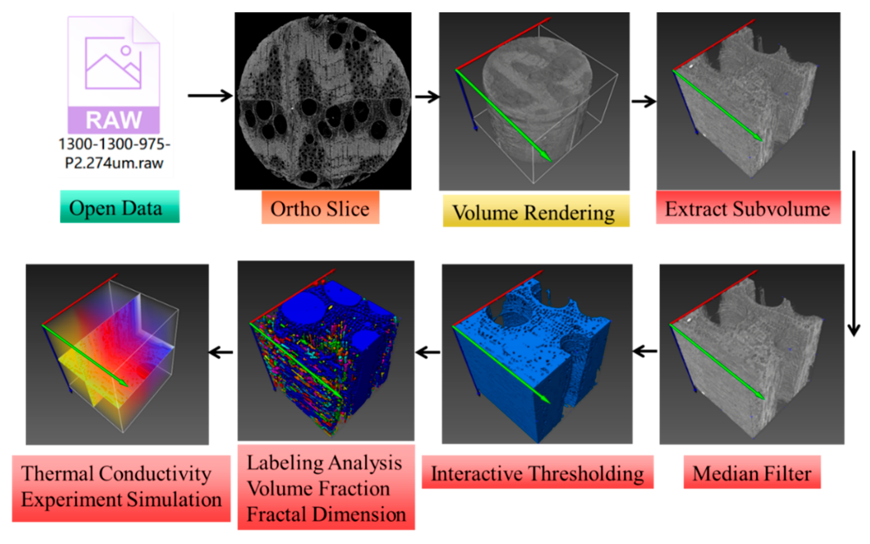
2.3.1. Digital Image Processing Method

The data obtained from the XCT scans of the oak samples were processed using Avizo Fire 8.1 software to simulate and solve for the sample’s heat transfer and fluid flow properties. The data were imported into Avizo Fire 8.1 software, where the oak wood samples were sliced for observation. (1) Slice observation involved three-dimensional visualization of the data from each layer of the oak sample. (2) After three-dimensional rendering, the dataset was analyzed on the 3D structure. (3) The purpose of image cropping was to select arbitrary regions of the sample’s 3D structure for data analysis, enhancing computational efficiency and accuracy. The selected slices and cropped regions needed to include clear images of macroscopic structures such as wood rays, vessel pores, earlywood, latewood, and thin-walled tissues. (4) To ensure the accuracy of the 3D structural images of the sample, the noise filtering stage can eliminate the effects of environmental factors and equipment noise from the measurements. The purpose of image cropping is to control the variables and reduce the amount of computation. To ensure the accuracy of the 3D structural images of the samples, Median Filter processing was used to eliminate the effects of environmental factors and equipment noise in the measurements. (5) Threshold segmentation can differentiate between the wood cell walls (wood matrix) and the pores. The pores are extracted more accurately with a threshold value of 18,000. In this experiment, the threshold was consistently set to 18,000 to control for variables. (6) During the parameter analysis process, labeling analysis, volume fraction, and fractal dimension commands are typically used to label the pores, calculate pore quantities, pore size distribution, volume fractions, and fractal dimensions. The specific experimental procedure is illustrated in Figure 2.
The calculation of the fractal dimension in the software is the Box-counting method. To calculate the dimension of a fractal S, the fractal is placed on a uniformly divided grid, and the minimum number of grids needed to cover the fractal is calculated. The counting box dimension is calculated by gradually refining the grid to see the change in the number of required coverings. Suppose that the total number of lattices that divide the space into N lattices when the lattice’s side length is ε, then the counting box dimension is obtained as follows [28]:
d i m b o x S lim ε 0 log N ε log 1 ε

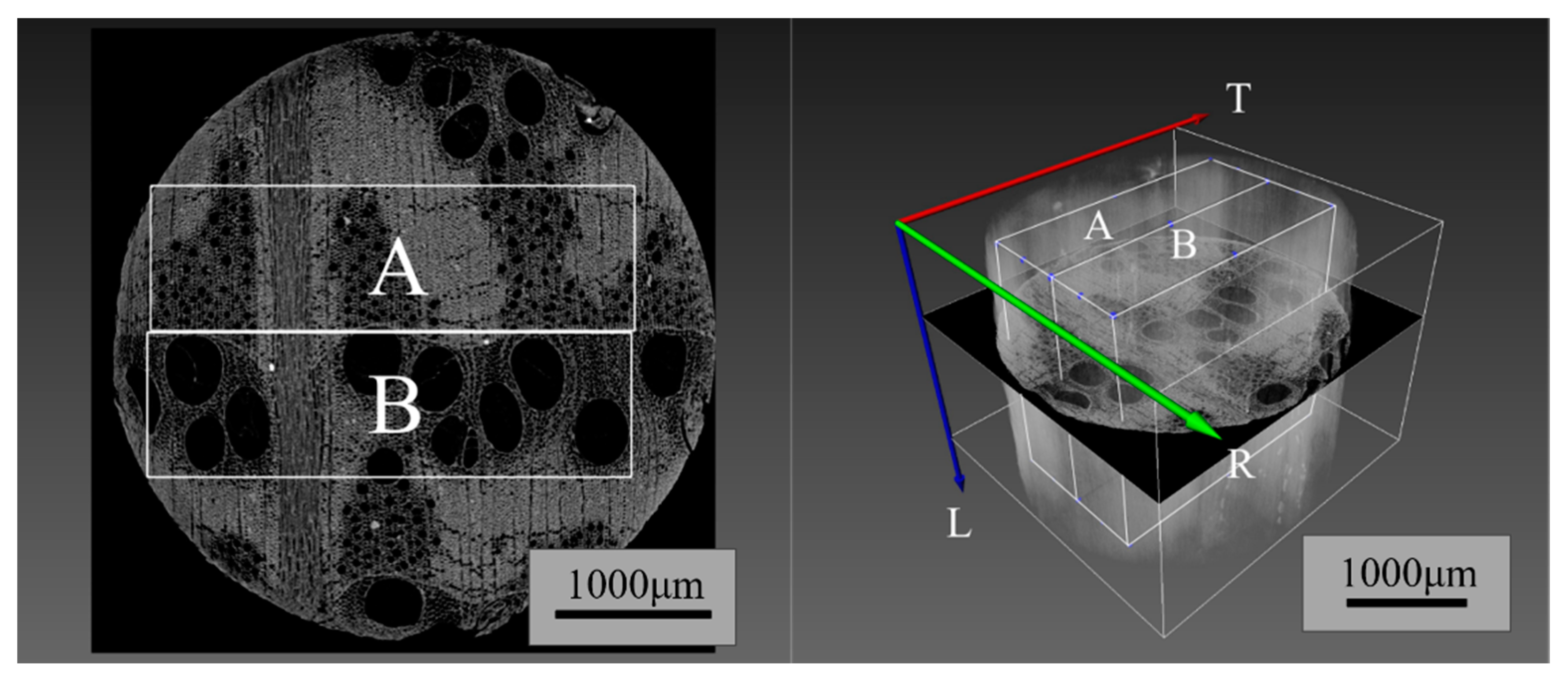
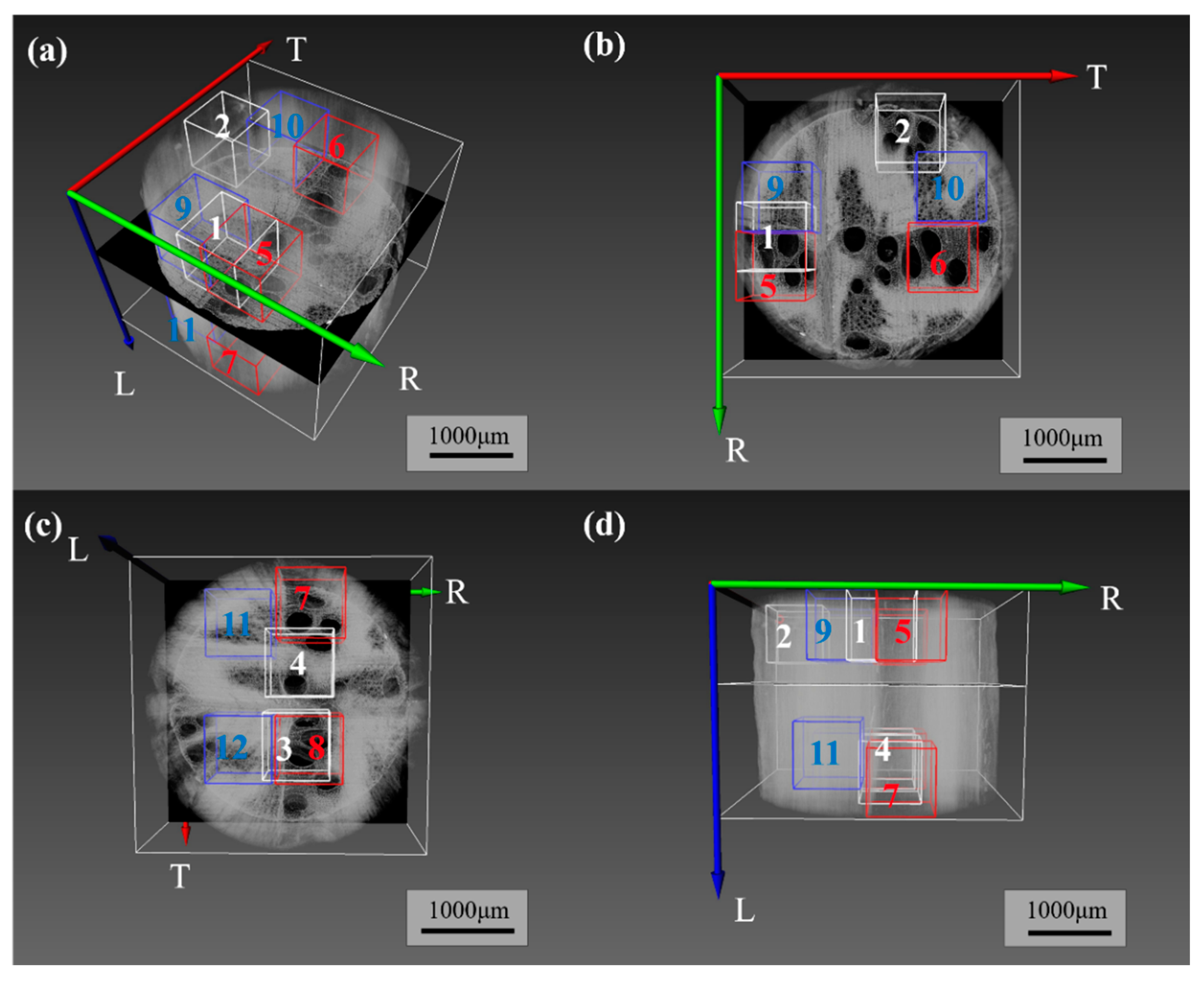
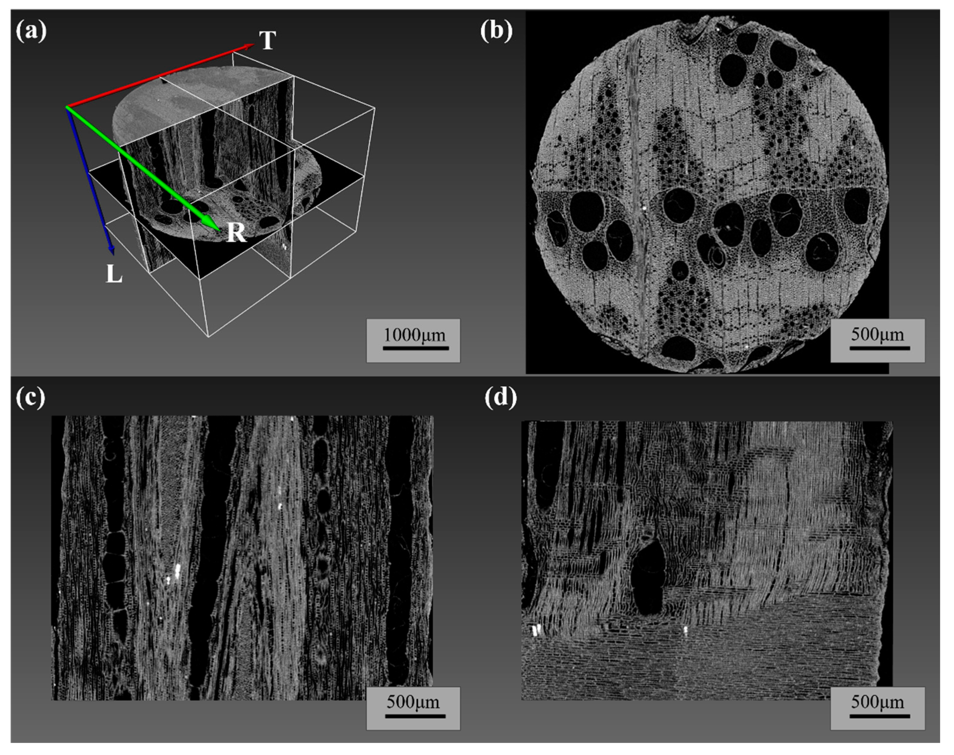
2.3.2. Selection of Characteristic Pore Areas in Wood

Using digital image processing techniques, the physical properties of the wood pore structure were detected and quantitatively characterized, including porosity, pore size and distribution, and fractal dimension. Due to the biological characteristics of wood, there are significant differences between earlywood and latewood. Therefore, this study evaluated the three-dimensional structural parameters of earlywood, latewood, and the oak sample as a whole (OSW), separately. As shown in Figure 3, the following three regions of the oak sample were selected for quantitative analysis: the earlywood zone, the latewood zone, and the overall sample. The dimensions of the latewood zone (A) and the earlywood zone (B) were 1000 × 300 × 975 pixels, while the dimensions of the overall sample (A + B) were 1000 × 600 × 975 pixels.

2.3.3. Effective Thermal Conductivity Simulation

Using the Xlab Thermo Pack module in Avizo, the effective thermal conductivity of the oak was calculated based on the XCT-reconstructed real geometry. This was performed with pure diffusion (without convection or radiation). In order to make the calculation feasible, 12 three-dimensional substructures (numbered 1–12) with dimensions of 300 × 300 × 300 pixels each were selected from the OSW, as shown in Figure 4. At the boundary between earlywood and latewood, regions 1–4 represent the overall sample, regions 4–6 represent earlywood, and regions 5–8 represent latewood. The effective thermal conductivity of wood cell walls was set at 0.654 W/(m∙K), while the thermal conductivity of air was set at 0.023 W/(m∙K) [29,30]. The temperature difference between the two parallel boundaries along the heat transfer direction was set to 40 K, with an inlet temperature of 333 K and an outlet temperature of 293 K, while other conditions were set to adiabatic. The simulation experiments were conducted on a computer equipped with an Intel® Core™ i7-8565U CPU @ 1.80 GHz and 16 GB of RAM. The simulations for the tangential, radial, and axial directions of the sample took 12 h. During each direction’s thermal conductivity simulation, temperature field data were obtained. The effective thermal conductivity of the wood during the simulation was calculated as follows [31]:
λ = Q d A T x A
where λ represents the effective thermal conductivity from the simulation results (W/(m∙K)), ∂T/∂x is the temperature gradient along the heat transfer direction, Q is the heat flux along the heat transfer direction (W/m2), and A is the heat transfer areas (m2).

2.3.4. Pore Size Determination

Pore size distribution is another critical parameter for assessing pore structure. This study employed a stratified pore size calculation method. By determining the pore size distribution for each layer, the overall pore size distribution could be derived using the following equation:
f d ;   μ ,   σ = 1 2 π σ d e x p l n d μ 2 2 σ 2
where d represents the pore diameter (μm), μ is the average pore diameter (μm), and σ is the standard deviation.
In summary, our expectation is to obtain a correlation between fractals and thermal conductivity for the purpose of evaluating the thermal conductivity of wood using fractal dimensions.

3. Results and Discussion

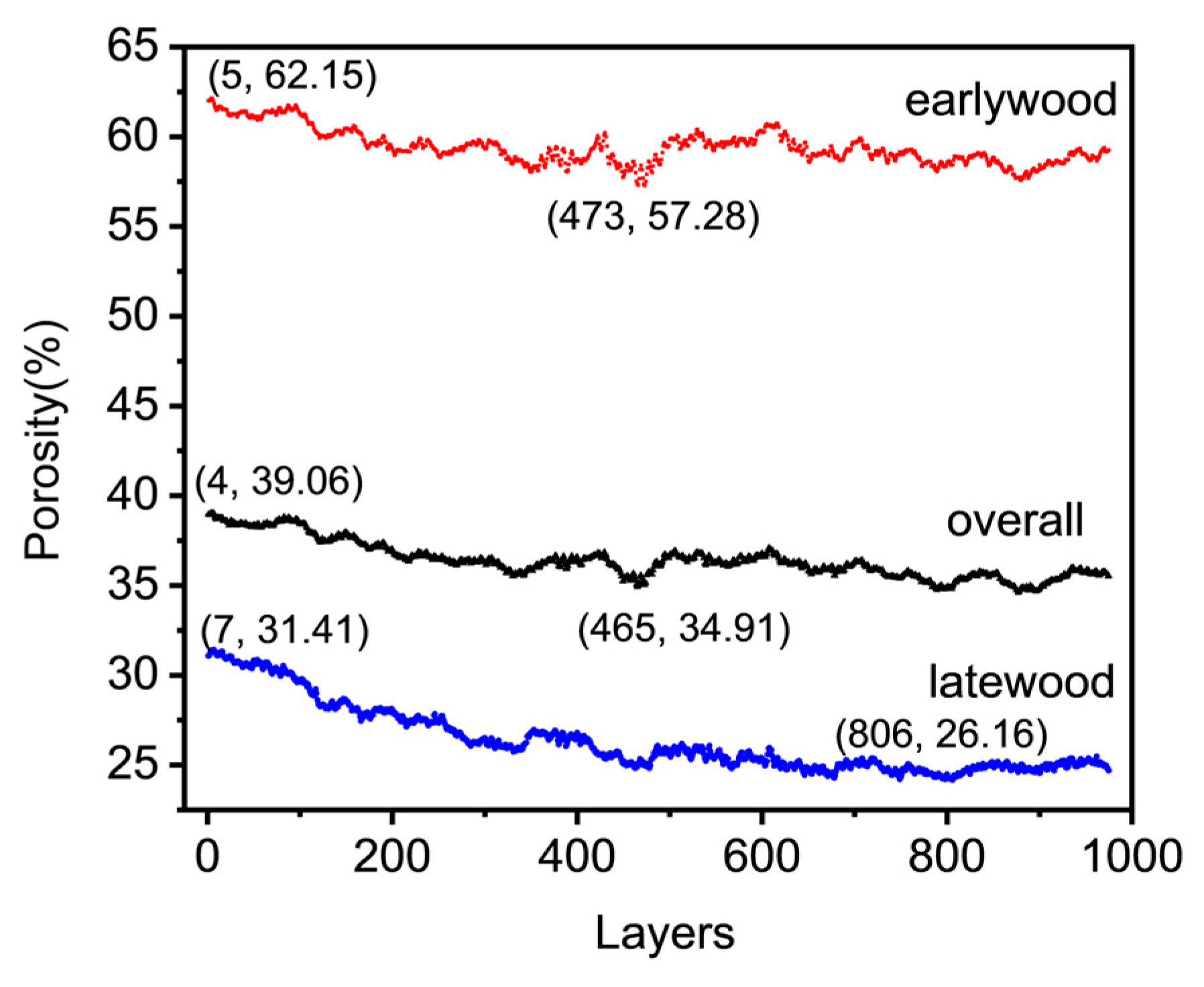
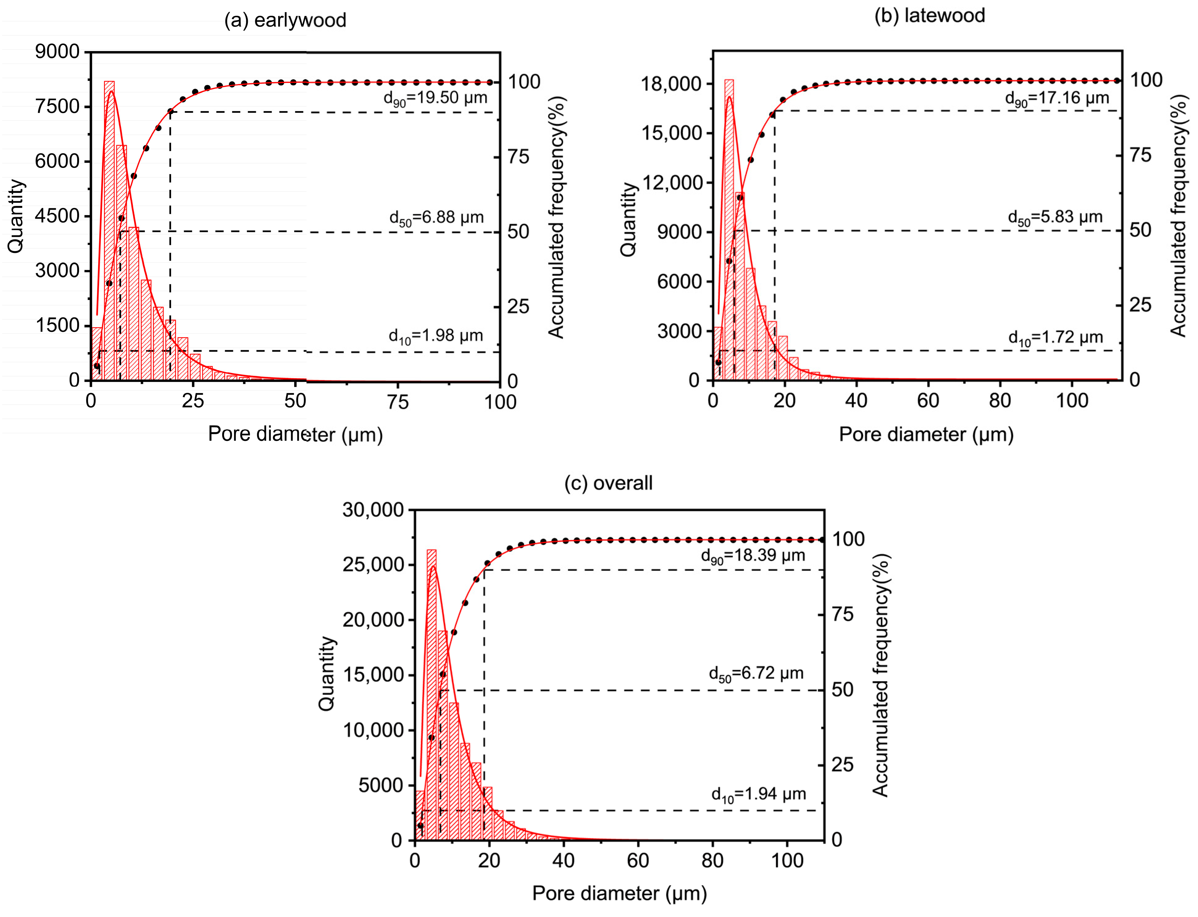
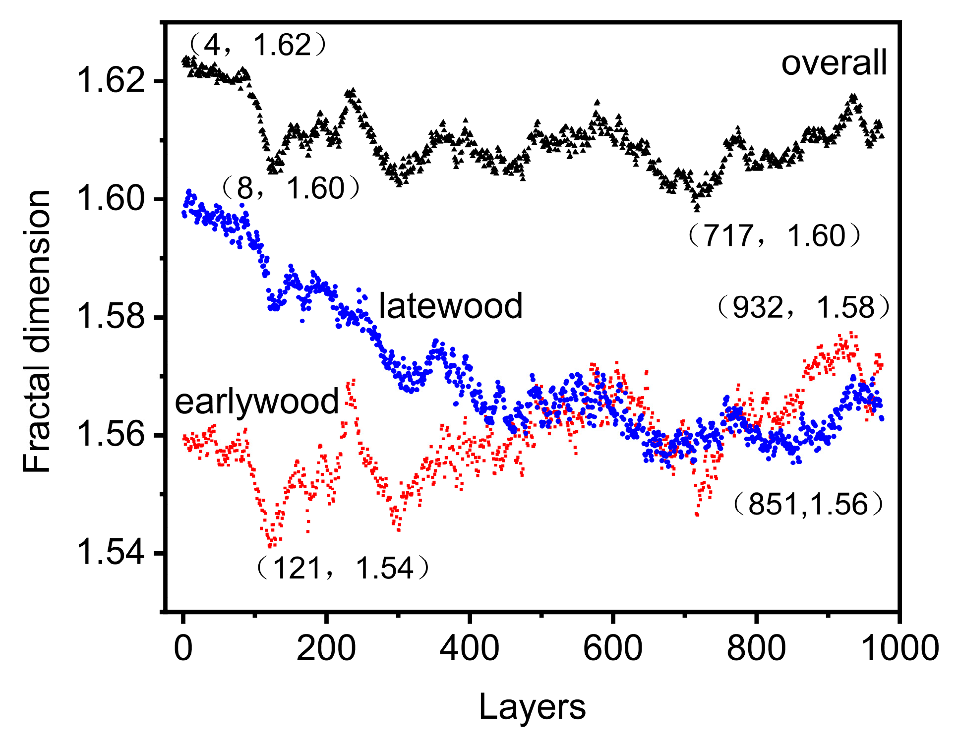
3.1. Pore Structure and Parameters

Wood pores can be classified from macroscopic to microscopic as macropores > 2 μm, 2 μm < mesopores < 10 μm, and micropores <10 μm, while XCT technology can characterize the pore structure of wood with resolution down to the micrometer scale [32]. Figure 5 displays micrometer-scale images of the oak sample’s T-R-L cross-sections and OSW obtained using XCT technology. In these images, the gray and black areas correspond to the wood matrix (cell walls) and pores, respectively. To thoroughly investigate the impact of the three-dimensional structure of the oak sample on its 3D porosity, clear images containing wood rays, vessel pores, earlywood, latewood, and thin-walled tissues were selected. Cross-sections, tangential sections, and radial sections were obtained from layers 487, 650, and 650, respectively, as shown in Figure 5.
Porosity is one of the primary factors referred to when assessing the structural characteristics of wood. It is defined as the ratio of pore volume to the total sample volume and is significantly influenced by the macroscopic features of the wood. This study used XCT scanning to obtain micrometer-scale 3D structural images of the oak sample and analyzed the porosity layer by layer. Figure 6 displays the porosity of the oak sample along the axial direction for each layer. The porosity ranges for earlywood, latewood, and the overall sample were 57.28–62.15%, 26.16–31.41%, and 34.91–39.06%, respectively. The average porosities were 59.41%, 26.4%, and 36.39%, with standard deviations of 0.95, 1.86, and 1.01, respectively. The results indicated that the porosity of the earlywood in the oak sample was significantly higher than that of the latewood. The variation in porosity between layers was attributed to the radial arrangement of vessel pores and the axial arrangement of thin-walled tissues within growth rings. The porosity calculated in this study was nearly identical to the value measured by Guo et al. [23] using XCT, which was 37.6%. The result was slightly lower than the porosity measured by Zhao et al. using MIP (44.26%). This discrepancy is due to the fact that the applied pressure in mercury intrusion can collapse the wood cell walls, creating artificial fissures [19]. Additionally, mercury intrusion may suffer from incomplete penetration into internal pores if the pressure is insufficient, increasing error. Extractives might also block pores, preventing mercury from penetrating. These issues do not affect XCT measurements. Additionally, the resolution of the XCT system and the accuracy of the matrix and pore segmentation algorithms have an impact [33].
The cumulative and histogram plots of the pore size distribution for oak are shown in Figure 7. The pore size distributions for earlywood, latewood, and the overall sample exhibited a log-normal distribution, with R2 values of 0.99. The average pore diameters for earlywood, latewood, and the OSW were 10.56, 9.53, and 10.21 μm, respectively. The results indicated that the average pore diameter of earlywood was larger than that of latewood. As shown in the cumulative plot in Figure 7, the values of d10 were 1.98, 1.72, and 1.94 μm, respectively. d10 refers to the pore size at which 10% of the cumulative pore size distribution is smaller, meaning that 10% of the pores have a size smaller than this value. The values of d50 were 6.88, 5.83, and 6.72 μm, respectively. d50 represents the pore size at which 50% of the cumulative pore size distribution is smaller, also known as the median pore diameter. This is a characteristic value that precisely divides the material’s pore sizes into two equal parts. The values of d90 were 19.50, 17.16, and 18.39 μm, indicating that 90% of the pore sizes were smaller than these values. In conjunction with Figure 5b, it can be observed that earlywood contained some large pores around 200 μm; yet, the output data did not show any pores larger than 100 μm. This suggests that the image processing software may have classified these large pores as part of the wood matrix. It should be noted here that we will gradually improve this problem in subsequent studies. Future studies will involve attempts such as grayscale preprocessing during image processing, which may potentially enhance the differentiation between the matrix and pores. The image processing software included with the XCT system utilized a sphere–cylinder model for equivalent calculations.
Based on the anatomical characteristics of wood, the pores within it primarily consist of cell lumina (10–50 μm), pits (2–15 μm), and micropores in the cell walls (2–5 nm) [34]. However, micropores are typically difficult to detect. As shown in Figure 7, the measured pores were mainly pits and cell lumina, with the number of pits being significantly greater than the number of cell lumina.
The fractal dimension is a measure of the irregularity of complex shapes. As shown in Figure 8, the fractal dimension varied with the number of layers in the three-dimensional structure of the oak sample. The surface fractal dimensions for earlywood, latewood, and the OSW three-dimensional structure ranged from 1.54 to 1.58, 1.56 to 1.60, and 1.60 to 1.62, respectively. The average values were 1.56, 1.57, and 1.61, respectively, with standard deviations of 0.0073, 0.012, and 0.005. The fractal dimensions of the OSW three-dimensional structure were 2.60, 2.61, and 2.64. There was only a slight linear correlation between the fractal dimensions and porosity in both earlywood and the OSW three-dimensional structure of the oak sample. The fractal dimension of earlywood showed a negative linear correlation with porosity (R2 = 0.49), while the fractal dimension of the OSW exhibited a positive linear correlation with porosity (R2 = 0.43). In contrast, the increase in fractal dimension for latewood was highly correlated with the increase in porosity, with an R2 value of 0.96. The axial cell arrangement in latewood is more orderly compared to earlywood, which better aligns with the self-similarity required by fractal dimensions. In summary, the findings indicated that, as the self-similarity of the wood structure increased, the correlation between porosity and fractal dimension became stronger, and the relationship between the two was positively correlated. The calculated surface fractal dimension in this study was similar to the value obtained by Zhao et al. [24] for larch, which was 1.779. However, the fractal dimension for OSW in this study significantly differed from the OSW fractal dimension reported by Dessie (2.87–2.96) [35], but it aligned with the fractal dimension of mesopores (radius 5000–100 nm). The reason was that larger pores in wood implied a more complex pore structure. During the image processing phase, the analysis software may have inadvertently classified the largest vessel pores as part of the wood matrix. This resulted in the porosity and fractal dimension measurements being lower than their actual values.

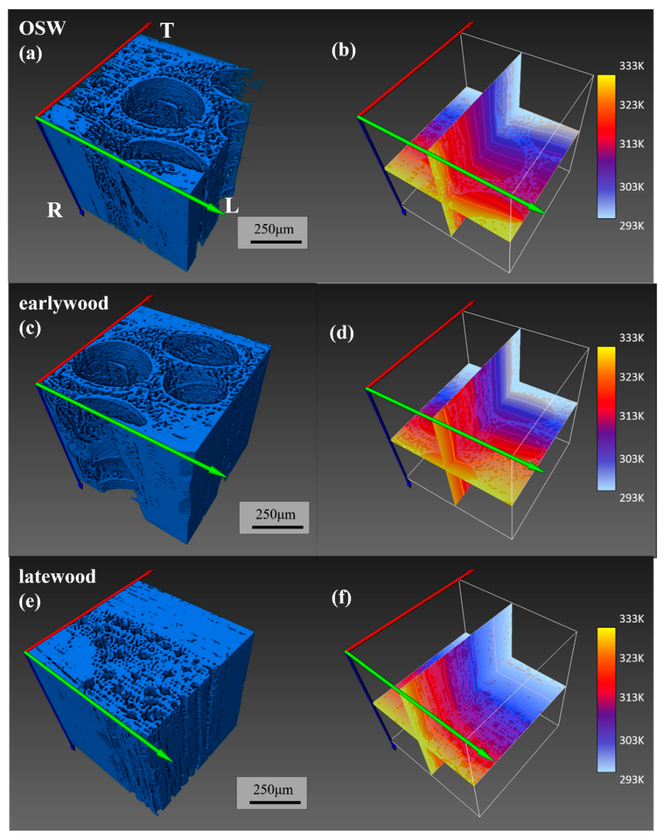
3.2. Heat Transfer Simulation and Validation

The XCT simulation method allowed for the estimation of the effective thermal conductivity and the internal temperature field of the oak samples. Figure 9 displays the temperature contours and isothermal sections for the TR and TL planes when the effective thermal conductivity simulated in the T direction was constant, for three substructures (1, 5, and 9) on the three-dimensional structure. The temperature ranged from 333 K to 293 K, with yellow to white representing this gradient. The results demonstrated that the porous structure had a significant impact on thermal conductivity. Heat was transferred more efficiently through the solid phase with higher thermal conductivity, while the presence of pores impeded the heat transfer process. Latewood exhibited stable heat transfer with relatively straight isotherms, whereas earlywood showed curvature in the isotherms due to the presence of vessel pores. A comparison of substructures 5 and 9 revealed that latewood lacked vessel pores and had more axial voids, with a more uniform pore distribution compared to earlywood. This confirmed the decisive influence of large pores on thermal conductivity.
Table 1 presents the effective thermal conductivity coefficients for substructures 1–4 in three directions. The average values obtained from the simulations were compared with experimental and reference values [36] and are depicted in a box plot (see Figure 10). The average effective thermal conductivity coefficients in the T, R, and L directions were 0.178, 0.189, and 0.282 W/(m∙K), respectively. These findings align with the literature, which states that L-direction thermal conductivity is greater than R-direction, and R-direction is greater than T-direction thermal conductivity [11]. Due to the anisotropy of wood, the effective thermal conductivity is influenced by the macrostructural characteristics in each direction. Comparing the theoretical simulation averages with the measured values, the errors (Error = (Measured Value − Calculated Value)/Measured Value × 100%) were 1.14%, 0.53%, and 9.3% for the three directions, respectively. The results indicated that the XCT-based thermal simulations were accurate for the T-direction and R-direction effective thermal conductivities but showed significant discrepancies for the L-direction effective thermal conductivity. This was due to the digital image processing, where smaller L-direction attachment pores were designated as part of the matrix, leading to an inability to precisely predict the L-direction effective thermal conductivity. Additionally, the anisotropic nature of wood and the presence of extractives within oak pores also influenced the experimental outcomes. The tangential and radial thermal conductivities were primarily influenced by large pores, with a lesser impact observed. The average thermal conductivities for earlywood in the three directions were 0.145, 0.154, and 0.234 W/(m∙K), respectively, while for latewood, they were 0.356, 0.422, and 0.478 W/(m∙K). The thermal conductivities followed the order axial > radial > tangential. The thermal conductivity of latewood was significantly higher than that of earlywood, which was related to porosity and is explored in the next section.

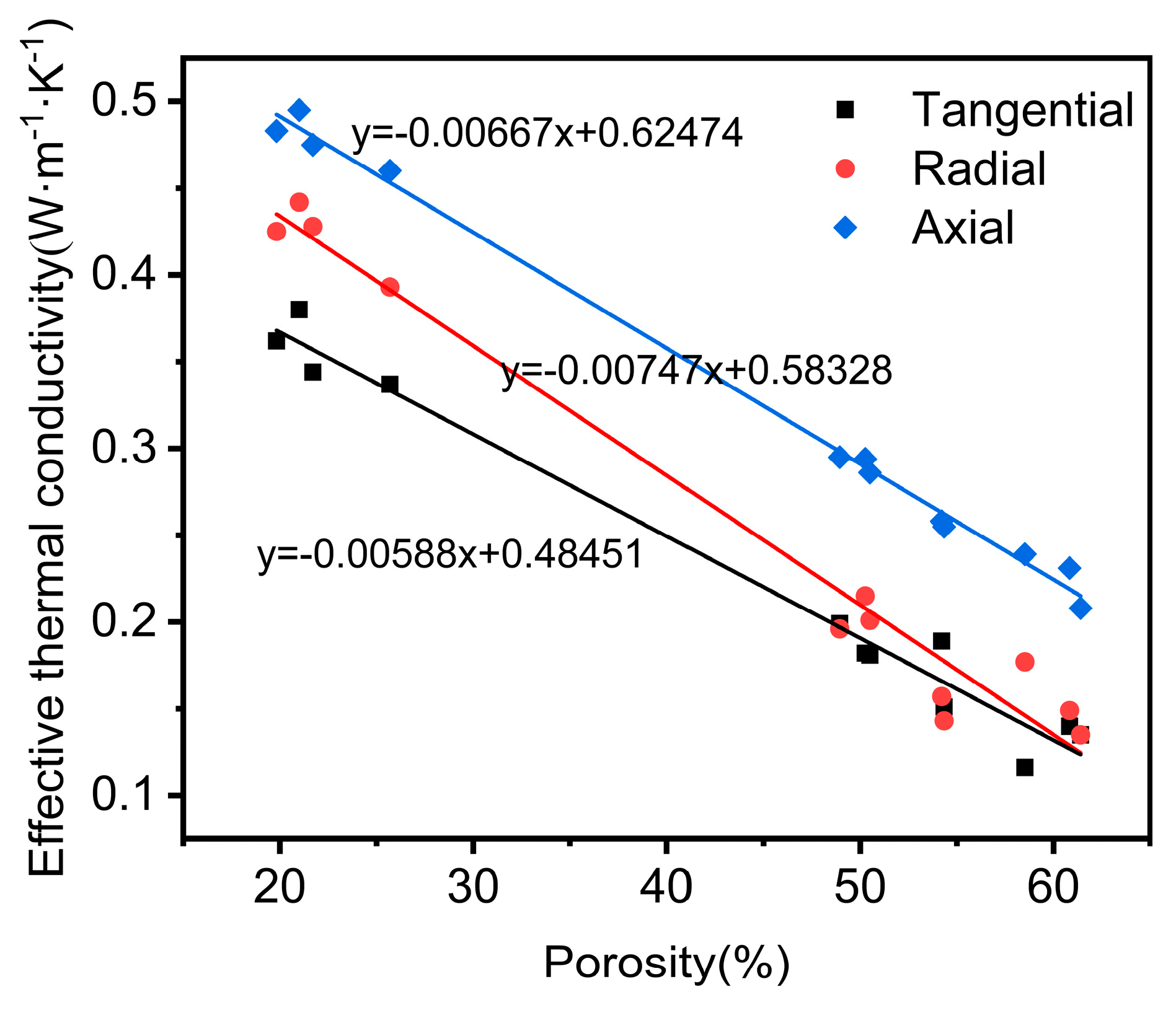
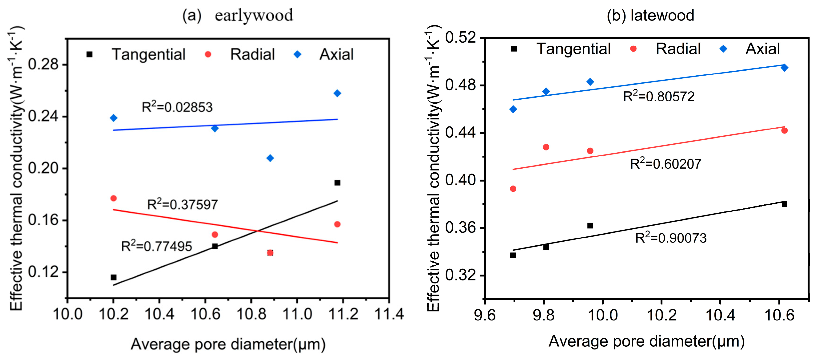
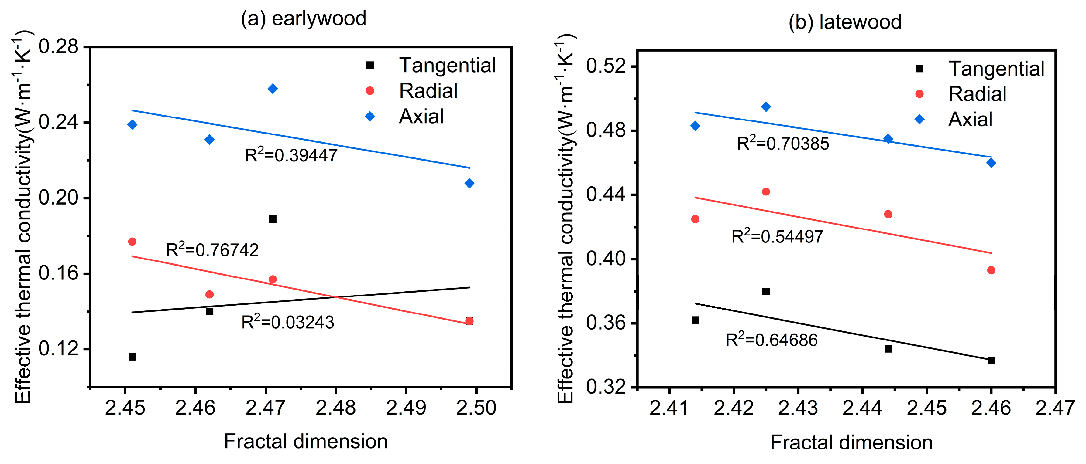
3.3. Relationship Between Pore Structure and Thermal Conductivity

Figure 11 demonstrates a linear relationship between the porosity of the oak samples and their effective thermal conductivity. As porosity increases, the effective thermal conductivity decreases. The R2 values for the fitted curves of the oak samples in the tangential, radial, and fiber directions were 0.98, 0.98, and 0.99, respectively. As a wood material, heat flux must traverse both the solid matrix (cell walls) and the pores within the wood. The thermal conductivity of air within the pores is significantly lower than that within the solid material. Consequently, an increase in porosity results in a decrease in the thermal conductivity of the oak samples. According to the analysis models by Liu and Zhao [37], as porosity increases, the thermal conductivity of the porous structure approaches that of the gas within the pores. This finding is consistent with the simulation results, which indicate that the thermal conductivity follows the order of earlywood < OSW < latewood.
Figure 12 illustrates the relationship between the average pore diameter and the thermal conductivity of earlywood and latewood. However, large pores have a decisive impact on the thermal conductivity of wood, and the average pore diameter of earlywood does not significantly reflect the effect of vessel pores on heat conduction. In contrast, as the average pore diameter increased in latewood, the effective thermal conductivity also increased. The average pore diameter accounted for at least 60% of the variability in the simulated thermal conductivity of latewood. The fitting performance for the fiber direction and tangential direction was notably good, with R2 values exceeding 0.8. The results indicated that using the average pore diameter to describe the thermal conductivity of wood is feasible for latewood or coniferous wood with uniform pore size distribution. However, Liu and Zhao’s [37] model results showed that, as pore size decreases, the effective thermal conductivity remains nearly constant. This may be attributed to the discrepancy between the actual structure of the vessels and the model; vessels do not represent an ideal porous structure. Instead, they exhibit an elliptical shape in the cross-section, with openings at both ends of the short axis and vessel membranes along the long axis [34]. Section 3.1 revealed that vessel pores were thinner areas of secondary cell walls and served as conduits for moisture and other substances within wood cells. This implied that vessel pores could not be neglected when simulating heat transfer through the wood’s porous structure. The impact of vessel pore structure on heat transfer requires more in-depth investigation. Therefore, when conducting heat transfer simulations using the actual pore structure of wood, special attention should be given to the influence of vessel pores. Additionally, due to the impact of large pores, pore diameters needed to be categorized into several ranges for relevant analysis. Future research could employ grey relational theory for further study [38].
The simulated results for the effective radial thermal conductivity of earlywood exhibited a weaker correlation with the average pore diameter. This was attributable to the fact that radial cell growth was uneven due to seasonal variations in climate temperature and precipitation. In contrast, wood cells along the tangential and fiber directions developed under similar climatic conditions at the same time, resulting in minimal variation. Consequently, when heat flowed through the wood in different directions, the radial heat flux traversed a more complex and variable structure.
Figure 13 illustrates the relationship between the fractal dimension of latewood and earlywood and their effective thermal conductivity. As the fractal dimension increased, it correspondingly reduced the effective thermal conductivity, though the correlation was relatively weak, with R2 values ranging from 0.39 to 0.70. In other words, as the pore structure became more complex, heat transfer became more difficult, resulting in a lower thermal conductivity. The correlation between the fractal dimension of earlywood and its effective thermal conductivity was relatively weak. This may be due to significant errors associated with the box-counting method or potentially due to an insufficient sample size. The ideal method for calculating fractal dimension remains controversial, and no universal calculation method currently exists [39]. This study selected oak as the target species, characterized by the following distinct anatomical differences: earlywood vessels are larger in diameter and arranged loosely with thinner cell walls, whereas latewood vessels are smaller and densely packed with thicker cell walls. Earlywood rays are broader and more dispersed compared to the narrower, tightly organized latewood rays. We hypothesized that when cell walls are excessively thin, the correlation between fractal dimension and thermal conductivity becomes less pronounced. This suggests that selecting species with thicker earlywood cell walls could enhance the fractal dimension–thermal conductivity relationship due to strengthened pore–wall interfacial heat transfer. Additionally, while this study identified a correlation between fractal dimension and thermal conductivity, further theoretical and experimental work is needed to develop specific methods for assessing wood using this parameter.

4. Conclusions

Using XCT technology, this study investigated the three-dimensional structure of oak wood and its relationship with thermal conductivity, focusing on earlywood and latewood. This study examined the samples’ porosity, pore size and distribution, and fractal dimension. Thermal conductivity simulations of the oak samples’ three-dimensional structure were conducted and validated using the transient plane source (TPS) method. Finally, the impact of the oak wood’s pore structure on thermal conductivity was evaluated. The main conclusions are as follows:
(1) In order to conduct the thermal conductivity research based on the simulation of the real structure of wood, the X-ray computed tomography (XCT) was combined with digital image processing methods, and the pore parameters of wood as well as their relationship with thermal conductivity were obtained. Within the scope of this study, the porosity, average pore diameter, and fractal dimension values for the oak samples were 36.39%, 10.21 μm, and 2.64, respectively. There is little difference in the fractal dimension between earlywood and latewood, and the overall fractal dimension is relatively large. When the self-similarity of the wood structure is higher, the correlation between the porosity and the fractal dimension is stronger, and it is a positive correlation between them.
(2) The simulation results indicated that the thermal conductivity of the oak samples was greatest in the fiber direction, followed by the radial and tangential directions, with latewood exhibiting higher effective thermal conductivity than earlywood. The heat transfer simulations based on XCT might have some axial deviations due to limitations in CT resolution and threshold segmentation methods, which require further refinement. Overall, however, the method provided relatively accurate estimates of the effective thermal conductivity of oak wood.
(3) Porosity was a major factor influencing the thermal conductivity of wood. There was a correlation between the average pore diameter, fractal dimension, and effective thermal conductivity of the oak samples. Compared with the ideal homogeneous model, the pore diameter of latewood is not irrelevant to the effective thermal conductivity. Therefore, the research on the thermal conductivity of multi-scale pore structures is of crucial importance to the study of the thermal conductivity of wood. Among the primary pores were pits and cell cavities, with pit pore structure warranting further attention in future studies on heat transfer. Additionally, the correlation for earlywood was weaker, and its behavior required further investigation.
This study has certain limitations. Due to the unique characteristics of wood, that is, there is no completely identical wood structure. When investigating the influence of one parameter, it is impossible to keep other parameters unchanged. Therefore, we can only try our best to reduce the impact of parameter changes and select the parts with similar remaining parameters for research. In future research, convection and radiation heat transfer should be considered, since in large pores these forms of heat transfer become important.

Author Contributions

Conceptualization, writing—review and editing, and funding acquisition, J.Z.; methodology, formal analysis, and writing—original draft, B.C.; validation, J.L.; data curation, J.Y.; investigation, L.Y.; software and formal analysis, Y.L.; resources, X.C.; conceptualization, writing—review and editing, and supervision, Y.C. All authors have read and agreed to the published version of the manuscript.

Funding

This research was supported by National Natural Science Foundation of China (No. 32271786).

Data Availability Statement

Data is contained within the article.

Conflicts of Interest

The authors declare no conflicts of interest.

References

  1. Zhao, J.; Guo, L.; Cai, Y. A novel fractal model for the prediction and analysis of the equivalent thermal conductivity in wood. Holzforschung 2021, 75, 702–711. [Google Scholar] [CrossRef]
  2. Altay, C.; Ozdemir, E.; Baysal, E.; Ergun, M.E.; Toker, H. Physical, mechanical, and thermal characteristics of alkaline copper quaternary impregnated oriental beech wood. Maderas Cienc. Tecnol. 2024, 26, 1–10. [Google Scholar] [CrossRef]
  3. Birinci, A.U.; Demir, A.; Ozturk, H. Comparison of thermal performances of plywood shear walls produced with different thermal insulation materials. Maderas Cienc. Tecnol. 2022, 24, 1–12. [Google Scholar] [CrossRef]
  4. Ding, H.; Zhao, L.; Yan, J.; Feng, H.-Y. Implementation of digital twin in actual production: Intelligent assembly paradigm for large-scale industrial equipment. Machines 2023, 11, 1031. [Google Scholar] [CrossRef]
  5. Poletto, M. Effect of extractive content on the thermal stability of two wood species from brazil. Maderas Cienc. Tecnol. 2016, 18, 435–442. [Google Scholar] [CrossRef]
  6. Yu, Z.L.; Qin, B.; Ma, Z.Y.; Gao, Y.C.; Guan, Q.F.; Yang, H.B.; Yu, S.H. Emerging bioinspired artificial woods. Adv. Mater. 2021, 33, 2001086. [Google Scholar] [CrossRef]
  7. Suleiman, B.; Larfeldt, J.; Leckner, B.; Gustavsson, M. Thermal conductivity and diffusivity of wood. Wood Sci. Technol. 1999, 33, 465–473. [Google Scholar] [CrossRef]
  8. Prałat, K. Research on thermal conductivity of the wood and analysis of results obtained by the hot wire method. Exp. Tech. 2016, 40, 973–980. [Google Scholar] [CrossRef]
  9. Wu, S.-S.; Tao, X.; Xu, W. Thermal conductivity of Poplar wood veneer impregnated with graphene/polyvinyl alcohol. Forests 2021, 12, 777. [Google Scholar] [CrossRef]
  10. Flity, H.; Jannot, Y.; Terrei, L.; Lardet, P.; Schick, V.; Acem, Z.; Parent, G. Thermal conductivity parallel and perpendicular to fibers direction and heat capacity measurements of eight wood species up to 160 °C. Int. J. Therm. Sci. 2024, 195, 108661. [Google Scholar] [CrossRef]
  11. Sova, D.; Porojan, M.; Bedelean, B.; Huminic, G. Effective thermal conductivity models applied to wood briquettes. Int. J. Therm. Sci. 2018, 124, 1–12. [Google Scholar] [CrossRef]
  12. Lagüela, S.; Bison, P.; Peron, F.; Romagnoni, P. Thermal conductivity measurements on wood materials with transient plane source technique. Thermochim. Acta 2015, 600, 45–51. [Google Scholar] [CrossRef]
  13. Hunt, J.F.; Gu, H. Two-dimensional finite element heat transfer model of softwood. Part I. Effective thermal conductivity. Wood Fiber Sci. 2006, 38, 592–598. [Google Scholar]
  14. Varnier, M.; Sauvat, N.; Ulmet, L.; Montero, C.; Dubois, F.; Gril, J. Influence of temperature in a mass transfer simulation: Application to wood. Wood Sci. Technol. 2020, 54, 943–962. [Google Scholar] [CrossRef]
  15. Díaz, A.R.; Flores, E.I.S.; Yanez, S.J.; Vasco, D.A.; Pina, J.C.; Guzmán, C.F. Multiscale modeling of the thermal conductivity of wood and its application to cross-laminated timber. Int. J. Therm. Sci. 2019, 144, 79–92. [Google Scholar] [CrossRef]
  16. Prochukhan, N.; Rafferty, A.; Canavan, M.; Daly, D.; Selkirk, A.; Rameshkumar, S.; Morris, M.A. Development and application of a 3D image analysis strategy for focused ion beam–Scanning electron microscopy tomography of porous soft materials. Microsc. Res. Tech. 2024, 87, 1335–1347. [Google Scholar] [CrossRef]
  17. Zhang, Y.; Lin, L.; Fu, F. High-permeability wood with microwave remodeling structure. Forests 2021, 12, 1432. [Google Scholar] [CrossRef]
  18. Plötze, M.; Niemz, P. Porosity and pore size distribution of different wood types as determined by mercury intrusion porosimetry. Eur. J. Wood Wood Prod. 2011, 69, 649–657. [Google Scholar] [CrossRef]
  19. Zhao, J.; Yang, L.; Cai, Y. Combining mercury intrusion porosimetry and fractal theory to determine the porous characteristics of wood. Wood Sci. Technol. 2021, 55, 109–124. [Google Scholar] [CrossRef]
  20. Cai, C.; Zhou, F.; Cai, J. Bound water content and pore size distribution of thermally modified wood studied by NMR. Forests 2020, 11, 1279. [Google Scholar] [CrossRef]
  21. Zhou, F.; Fu, Z.; Zhou, Y.; Zhao, J.; Gao, X.; Jiang, J. Moisture transfer and stress development during high-temperature drying of Chinese fir. Drying Technol. 2020, 38, 545–554. [Google Scholar] [CrossRef]
  22. Palombini, F.L.; Lautert, E.L.; Mariath, J.E.d.A.; de Oliveira, B.F. Combining numerical models and discretizing methods in the analysis of bamboo parenchyma using finite element analysis based on X-ray microtomography. Wood Sci. Technol. 2020, 54, 161–186. [Google Scholar] [CrossRef]
  23. Guo, L.; Cheng, H.; Chen, J.; Chen, W.; Zhao, J. Pore Structure Characterization of Oak via X-ray Computed Tomography. Bioresour. 2020, 15, 3053–3063. [Google Scholar] [CrossRef]
  24. Zhao, J.; Li, L.; Lv, P.; Sun, Z.; Cai, Y. A comprehensive evaluation of axial gas permeability in wood using XCT imaging. Wood Sci. Technol. 2023, 57, 33–50. [Google Scholar] [CrossRef]
  25. Andrä, H.; Dobrovolskij, D.; Engelhardt, M.; Godehardt, M.; Makas, M.; Mercier, C.; Rief, S.; Schladitz, K.; Staub, S.; Trawka, K. Image-based microstructural simulation of thermal conductivity for highly porous wood fiber insulation boards: 3D imaging, microstructure modeling, and numerical simulations for insight into structure–property relation. Wood Sci. Technol. 2023, 57, 5–31. [Google Scholar] [CrossRef]
  26. ISO 22007-2; Plastics-Determination of Thermal Conductivity and Thermal Diffusivity-Part 2: Transient Plane Heat Source (Hot Disc) Method. International Organization for Standardization (ISO): Geneva, Switzerland, 2008.
  27. Wu, K.F.; Cao, T.F.; Li, W.B.; Zhang, H.; Tang, G.H. Quantitative evaluation of the natural convection effect on thermal conductivity measurement with transient plane source method. Case Stud. Therm. Eng. 2023, 45, 102933. [Google Scholar] [CrossRef]
  28. Xie, H.; Zhang, Y.; Song, X. Fractal Geometry–Fundamentals and Applications of Mathematics; Chongqing Publishing House: Chongqing, China, 1991. [Google Scholar]
  29. Asako, Y.; Kamikoga, H.; Nishimura, H.; Yamaguchi, Y. Effective thermal conductivity of compressed woods. Int. J. Heat Mass Transf. 2002, 45, 2243–2253. [Google Scholar] [CrossRef]
  30. Maku, T. Studies on the Heat Conductin in Wood: The present study is a discussion on the results of investigations made hitherto by author on heat conduction in wood. Wood Res. Rep. Inst. Wood Res. Kyoto Univ. Jpn. 1954, 13, 1–80. [Google Scholar]
  31. Zhou, H.; Zhou, M.; Cheng, M.; Guo, X.; Li, Y.; Ma, P.; Cen, K. High resolution X-ray microtomography for the characterization of pore structure and effective thermal conductivity of iron ore sinter. Appl. Therm. Eng. 2017, 127, 508–516. [Google Scholar] [CrossRef]
  32. Everett, D.H. Manual of symbols and terminology for physicochemical quantities and units, appendix II: Definitions, terminology and symbols in colloid and surface chemistry. Pure Appl. Chem. 1972, 31, 577–638. [Google Scholar] [CrossRef]
  33. Elkhoury, J.E.; Shankar, R.; Ramakrishnan, T. Resolution and limitations of X-ray micro-CT with applications to sandstones and limestones. Transp. Porous Media 2019, 129, 413–425. [Google Scholar] [CrossRef]
  34. Petty, J. The aspiration of bordered pits in conifer wood. Proc. R. Soc. Lond. B Biol. Sci. 1972, 181, 395–406. [Google Scholar] [CrossRef]
  35. Tibebu, D.T.; Avramidis, S. Fractal dimension of wood pores from pore size distribution. Holzforschung 2022, 76, 967–976. [Google Scholar] [CrossRef]
  36. Liu, Y.; Zhao, G. Wood Science, 2nd ed.; China Forestry Publishing House: Beijing, China, 2012. [Google Scholar]
  37. Liu, H.; Zhao, X. Thermal conductivity analysis of high porosity structures with open and closed pores. Int. J. Heat Mass Transf. 2022, 183, 122089. [Google Scholar] [CrossRef]
  38. Javed, S.A.; Mahmoudi, A.; Khan, A.M.; Javed, S.; Liu, S. A critical review: Shape optimization of welded plate heat exchangers based on grey correlation theory. Appl. Therm. Eng. 2018, 144, 593–599. [Google Scholar] [CrossRef]
  39. Hatzikiriakos, S.; Avramidis, S. Fractal dimension of wood surfaces from sorption isotherms. Wood Sci. Technol. 1994, 28, 275–284. [Google Scholar] [CrossRef]
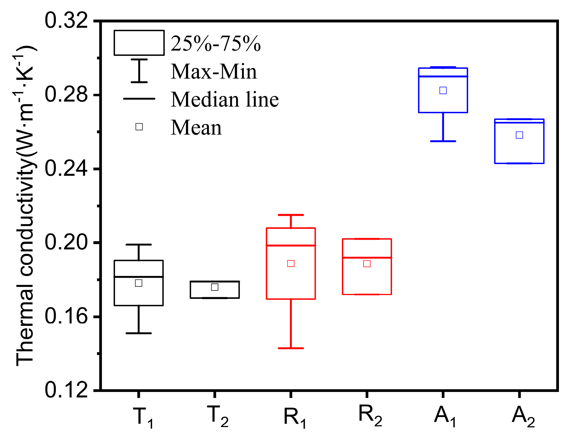
Figure 1. (a) XCT equipment; (b) TPS thermal constant analyzer and its testing procedure.
Forests 16 00834 g001
Figure 2. Labeling and processing based on XCT images.
Forests 16 00834 g002
Figure 3. Selection of areas for quantitative analysis.
Forests 16 00834 g003
Figure 4. Selection of substructures: (a) 3D side view; (b) selected area on the upper surface in the TR direction; (c) selected area on the lower surface in the TR direction; (d) selected area on the RL plane.
Forests 16 00834 g004
Figure 5. XCT image and trisection of the 3D structure of oak: (a) micron-scale image of the 3D structure of the specimen; (b) micron-scale image of the T-R oriented structure; (c) micron-scale image of the T-L oriented structure; (d) micron-scale image of the R-L oriented structure.
Forests 16 00834 g005
Figure 6. Porosity of oak face.
Forests 16 00834 g006
Figure 7. Pore size distribution of oak: (a) pore distribution of earlywood; (b) pore distribution of latewood; (c) overall pore distribution.
Forests 16 00834 g007
Figure 8. Fractal dimension of oak surface.
Forests 16 00834 g008
Figure 9. Simulation of the thermal conductivity of oak: (a,b) cross-sectional view and temperature distribution of the overall structure; (c,d) cross-sectional view and temperature distribution of the earlywood-containing portion; (e,f) cross-sectional view and temperature distribution of the latewood-containing portion.
Forests 16 00834 g009
Figure 10. Thermal conductivity box line diagram: (T1) tangential simulation, (T2) tangential experiment, (R1) radial simulation, (R2) radial experiment, (A1) axial simulation, (A2) axial experiment.
Forests 16 00834 g010
Figure 11. Relationship between porosity and thermal conductivity.
Forests 16 00834 g011
Figure 12. Relationship between average pore diameter and thermal conductivity: (a) earlywood, (b) latewood.
Forests 16 00834 g012
Figure 13. Relationship between fractal dimension and thermal conductivity: (a) earlywood, (b) latewood.
Forests 16 00834 g013
Table 1. Overall effective thermal conductivity of oak.
NumberTangential Thermal Conductivity (W/(m·K)) Radial Thermal Conductivity (W/(m·K))Axial Thermal Conductivity (W/(m·K))
10.151 0.143 0.255
20.181 0.201 0.286
30.199 0.196 0.295
40.182 0.215 0.294
Average/standard deviation0.178 (0.0199)0.189 (0.0314)0.282 (0.0185)
TPS experimental measurements0.1760.1880.258
Reference values0.1710.190 0.200
Disclaimer/Publisher’s Note: The statements, opinions and data contained in all publications are solely those of the individual author(s) and contributor(s) and not of MDPI and/or the editor(s). MDPI and/or the editor(s) disclaim responsibility for any injury to people or property resulting from any ideas, methods, instructions or products referred to in the content.

