Article

Trends and Influencing Factors of Summer Air Quality Changes in Four Forest Types

1
Key Laboratory of Carbon Sequestration and Emission Reduction in Agriculture and Forestry of Zhejiang Province, Zhejiang A&F University, Hangzhou 311300, China
2
Engineering Research Center of Bamboo Carbon Sequestration for State Forestry Grassland Administration, Hangzhou 311300, China
3
Institute of Ecological Civilization and Institute of Carbon Neutrality, Zhejiang A&F University, Hangzhou 311300, China
4
College of Forestry and Biotechnology, Zhejiang A&F University, Hangzhou 311300, China
5
Zhejiang Academy of Forestry, Hangzhou 310023, China
6
Faculty of Forestry, University of British Columbia, 2424 Main Mall, Vancouver, BC V6T 1Z4, Canada
*
Author to whom correspondence should be addressed.
These authors contributed equally to this work.
Forests 2025, 16(5), 833; https://doi.org/10.3390/f16050833 (registering DOI)
Submission received: 14 February 2025 / Revised: 13 May 2025 / Accepted: 14 May 2025 / Published: 17 May 2025
(This article belongs to the Section Forest Meteorology and Climate Change)

Abstract

:
Forest ecosystems are crucial in mitigating air pollution and improving air quality. Therefore, investigating the relationships between air quality, forest structure, and environmental factors in different forest types is of significant importance. This study conducted three months of continuous monitoring (June–September 2023) of air quality factors (particulate matter (PM2.5 and PM10), ozone (O3), and negative air ions (NAI)) and environmental factors (air temperature (TA), relative humidity (RH), light intensity (LI), and wind speed (WS)) in four subtropical forest types, along with vegetation characteristic surveys. The effects of forest structure and environmental factors on air quality were determined by correlation and multiple regression analysis. The results showed that the forest air quality is at its best in July during the summer season. Concentrations of particulate matter (PM) and ozone (O3) in mixed coniferous and broadleaf forests (MCB), as well as deciduous broadleaf forests (DB), are lower than those in moso bamboo forests (MB) and evergreen broadleaf forests (EB). The troughs of PM concentrations occur in the early morning (4:00–6:00), while the troughs of O3 concentrations occur in the early morning (4:00–6:00) and in the evening (18:00). NAI concentrations were highest in DB (1287 ions/cm3), followed by MCB (1187 ions/cm3), MB (896 ions/cm3), and EB (584 ions/cm3), with NAI concentrations peaking between 14:00 and 16:00. PM concentrations in forest air were primarily influenced by stand density (SD) and the Shannon–Wiener index of herbaceous layer (SWH) (p < 0.05); ozone concentrations were significantly affected by tree height (TH) and canopy density (CD) (p < 0.05); and NAI concentrations were primarily related to TH and diameter at breast height (DBH). Air particulate matter concentrations were negatively affected by TA and RH (p < 0.01), and ozone concentrations were negatively influenced by RH and WS and were positively influenced by TA. TA has a direct and significant positive effect on the NAI concentration (p < 0.01), and RH indirectly influences the changes in NAI concentration through its interaction with TA. This study provides new insights for vegetation optimization in forest parks and planning forest health-promoting activities for sub-healthy populations.

1. Introduction

Rapid economic development and urbanization have accelerated lifestyles, leading to severe environmental air pollution and a consequent rise in the number of sub-healthy individuals [1]. This has driven a growing public awareness of the critical importance of good air quality for physical health. Forest ecosystems are indispensable in mitigating air pollution and enhancing air quality, resulting in the increasing prominence of forest-based health and wellness activities. The effectiveness of forest-based health and wellness activities is closely linked to air quality, with particulate matter (PM), ozone (O3), and negative air ion (NAI) concentrations serving as key indicators [2,3]. PM is primarily categorized into fine particulate matter (PM2.5) and inhalable particulate matter (PM10) based on particle size, and high PM concentrations pose significant health risks, including respiratory and cardiovascular diseases [4]. Ozone is a specific irritant, and high ozone concentrations can damage the respiratory tract, exacerbate allergic reactions, and impair central nervous system cells [5]. NAI concentration is a significant indicator of good air quality and is known for its bactericidal, dust-reducing, and air-purifying effects [6]. To control air pollution, China implemented a second revision to the Air Pollution Prevention and Control Law in 2018. In addition to proposing methods such as reducing emissions of atmospheric pollutants and increasing the utilization rate of environmentally friendly renewable energy sources, forest vegetation was also recognized as a major tool for mitigating air pollution [7]. Currently, most urban residents choose to engage in activities within urban parks and green spaces. However, the relatively simple vegetation structure of these parks often fails to meet the needs of forest-based health and wellness [8], thereby failing to replicate the therapeutic effects experienced in natural forests. Consequently, research on air quality in healthy forests is urgently needed.
Forests, among the most abundant ecosystems on Earth, primarily improve air quality through the adsorption of airborne particulate matter, absorption of harmful gases, and release of negative air ions [9,10]. Forest vegetation, via physiological processes such as respiration and transpiration, reduces the internal forest temperature, subsequently altering relative air humidity and promoting the adsorption of PM onto plant leaves [11]. Factors such as plant leaf shape, size, surface roughness, and microscopic structure all influence the capacity of leaves to adsorb PM [12]. Furthermore, environmental factors such as temperature, humidity, and wind speed within the forest significantly influence the ability of leaves to retain PM. Plant leaves reduce ozone concentrations by absorbing O3 from the air through open stomata [13]. In terms of forest stand structure, the vertical structure of the plant community has a notable impact on PM concentration, with multilayered vegetation structures being more effective at reducing airborne PM levels than single-layered vegetation [14]. Related studies have demonstrated that tree diameter at breast height (DBH), leaf area index (LAI), and crown area have a significant effect on reducing PM concentrations [15]. In contrast, different vegetation compositions also produce various types of biogenic volatile organic compounds (BVOCs). Abundant vegetation can release substantial amounts of BVOCs, which in turn can lead to a significant increase in O3 concentration, indirectly impacting the generation of NAI [16].
Early research by Krueger [6] on negative air ions found that NAI can effectively inhibit the proliferation of viruses and bacteria, thereby providing an antibacterial and disinfecting effect. Furthermore, NAI has been shown to significantly improve cardiopulmonary endurance, reduce fatigue, and lower blood pressure [17]. The diurnal variation of NAI generally exhibits a bimodal or unimodal pattern, depending on the day-night cycle and environmental changes. Studies show that NAI concentrations are higher at midnight and early morning, lower at noon, and gradually increase in the afternoon, showing a “U”-shaped distribution [18]. Environmental factors exert a complex influence on NAI concentrations. As a primary factor affecting NAI concentrations, the temperature is influenced by relative air humidity, wind speed, and light intensity. Most studies have demonstrated a negative correlation between particulate matter concentration and NAI concentration, while relative air humidity and light intensity positively correlate with NAI concentration [19,20]. Due to variations in vegetation community composition and regional environmental conditions, NAI concentrations differ across various forest types. Related studies indicate that NAI concentrations are higher in mixed coniferous-broadleaved forests compared to pure broadleaved forests [21]. Furthermore, NAI concentrations within mixed coniferous-broadleaved forests are higher than in coniferous and deciduous broadleaved forests [22]. Recent studies have employed multiple regression analysis and random forest models to investigate the primary factors influencing NAI concentrations, identifying PM2.5, soil moisture, and relative air humidity as having a significant impact on NAI levels [23].
These studies have primarily focused on describing the relationships between air quality and environmental factors. However, research on the connection between air quality and forest stand structure remains limited, and there is a lack of comprehensive investigations into the synergistic effects of environmental factors and integrated analytical methods. To elucidate the overall impact of forest environments on air quality factors, this paper shifts from examining the effects of single environmental factors to exploring the coupled relationships between multiple environmental factors. Multivariate regression analysis and path analysis were employed to gain a deeper understanding of the interaction mechanisms among air quality, environmental factors, and forest stand structure, thereby offering a theoretical basis for optimizing vegetation and scheduling health and wellness activities in forest-based health centers.

2. Materials and Methods
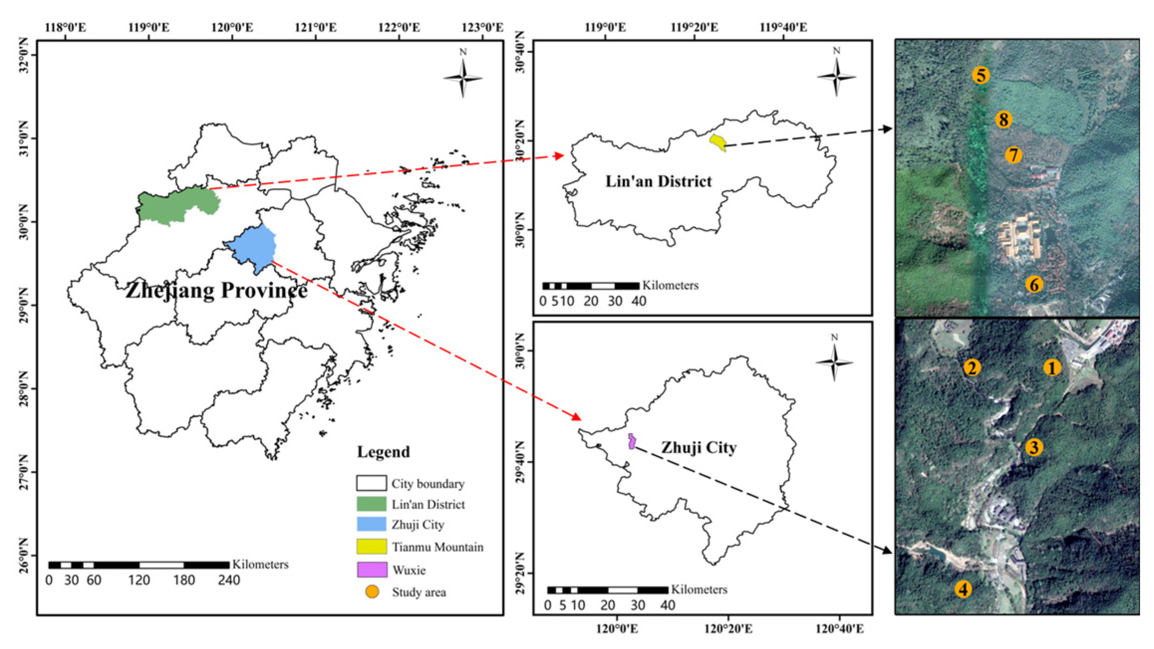
2.1. Study Area

This research was conducted in two scenic areas in Zhejiang Province with typical subtropical forests: Wuxie Scenic Area (120°02′–120°03′ E, 29°42′–29°45′ N) in Zhuji City and and Tianmu Mountain Scenic Area (119°24′–119°28′ E, 30°18′–30°24′ N) in Lin’an District (Figure 1). These two areas are 140 km apart and experience dry, cold winters and warm, humid summers with abundant rainfall. The average annual temperature is 15.2–16.2 °C, the average annual rainfall is 1390–1670 mm, and there are an average of 158.7–183.1 rainy days per year.
This study selected four typical forest types along the tourist trails of two scenic areas in Zhejiang Province for investigation. In the Wuxie Scenic Area, evergreen broad-leaved forests (EB) and moso bamboo plantations (MB) were chosen; in the Tianmu Mountain Scenic Area, mixed coniferous and broad-leaved forests (MCB) and deciduous broad-leaved forests (DB) were selected. Two sample plots were established within each forest type, resulting in eight sample plots (20 m × 20 m) across the four forest types. The selected sample site is located in the center of the forest, far away from the main roads of the scenic area and tourist concentration areas. Detailed information about the location of each monitoring point and the dominant plant communities is provided in Table 1 and Table 2. Understory vegetation was surveyed using a five-point sampling method within each sample plot. Five quadrats were established for both shrubs and herbaceous plants. Data collected included species and abundance of understory shrubs and herbs, shrub height density (SHD), and coverage of herb layer (CHL).

2.2. Observation Instruments

This study employed a fixed environmental factor meteorological monitoring station (ZX-AQI-L, Zhongxing EP Ltd., Shenzhen, China) to synchronously collect data on air temperature (TA), relative humidity (RH), light intensity (LI), wind speed (WS), fine particulate matter (PM2.5), inhalable particulate matter (PM10), ozone (O3), and carbon dioxide (CO2) within the sample plots over 24 h. The monitoring sensors were positioned at a height of 1.6 m, corresponding to the average human respiratory level. Data were recorded at a frequency of 1 min. Negative air ions (NAI) and HCHO were monitored using a portable air negative ion detector (WST-10D, IonWoston, Beijing, China), with data collected at a frequency of 10 s. Specific instrument parameters are detailed in Table 3.
Meteorological data were collected from 1 June to 1 September 2023. Before data acquisition, the meteorological monitoring station underwent a one-month operational testing period. NAI measurements were conducted on three clear, rain-free days between August and September 2023, with daily observations from 8:00 a.m. to 5:00 p.m. The portable negative air ion detector was calibrated and tested three days before use. Forest stand structure parameters, including average tree height (TH), average diameter at breast height (DBH), stand density (SD), and canopy density (CD), were obtained for each sample plot using a backpack LiDAR (LiBackpackDGC50, Digital Green Earth Technology Co., Ltd., Beijing, China).

2.3. Data Processing and Analysis

2.3.1. Data Processing

Due to the large variation in raw air quality data, conventional outlier detection methods were inadequate. This study utilized PyCharm 2023 to implement the filtering method from Shi et al. [23]: (1) Time-series data was screened for discontinuities and outliers caused by device malfunctions; (2) values of 0 were treated as outliers; (3) values that were greater than 5 times or less than 1/5 of adjacent values were treated as outliers; (4) sequences of six or more identical values were treated as outliers; and (5) values less than 10 were interpolated by averaging adjacent values, rounding to the nearest integer.
This study employed the Simpson diversity index and the Shannon–Wiener diversity index as evaluation metrics to assess understory vegetation species diversity. The Simpson diversity index for the shrub layer (SDS) and herbaceous layer (SDH), as well as the Shannon–Wiener diversity index for the shrub layer (SWS) and herbaceous layer (SWH), were calculated using the following formulas.
Simpson’s diversity index measures the probability that two randomly selected individuals belong to different species. It emphasizes dominance rather than species richness (number of species). Higher values of Simpson’s diversity index (D) indicate greater species diversity. The formula is as follows:
D = 1 i = 1 S ( P i ) 2
Shannon–Wiener diversity index quantifies biodiversity by measuring the entropy of species distribution. It integrates species richness and evenness (relative abundance). Higher values of the Shannon–Wiener index (H) indicate greater biodiversity, reflecting both richness and evenness. The formula is as follows:
H = i = 1 S P i ln P i
In these formulas, S is the total number of species in the sample plot, and Pi is the proportion of individuals of a given species compared to the total number of individuals of all species in the community.

2.3.2. Data Analysis

In this study, to examine the impact of environmental factors on the concentrations of air pollutants, Spearman’s correlation analysis was first conducted on the environmental factors and air pollutants. Then, using the daily average data as samples (n = 92), multiple regression equations between air pollutants and environmental factors were constructed, with PM2.5, PM10, and O3 as the dependent variables respectively, and TA, RH, WS, and LI as the independent variables. In the multiple regression equations between air quality factors and forest stand structure, TH, DBH, SD, SHD, CHL, CD, SDS, SDH, SWS, and SWH of 8 sample plots were selected as independent variables, respectively. When constructing the regression equations, we selected the stepwise regression method to construct the optimal regression model, which can effectively retain the most relevant variables and prevent the occurrence of overfitting and multicollinearity problems.
Previous studies have demonstrated that the Random Forest (RF) model can determine the influence degree of environmental factors on NAI [18,24]. In this study, the RF model and path analysis were selected to examine the influence degree of various environmental factors on the changes in NAI concentration. Using the ten-minute average data of each factor collected during the monitoring period as samples (n = 46), with the NAI concentration as the dependent variable and environmental factors including TA, RH, WS, LI, PM2.5, PM10, and O3 as the independent variables, a Spearman’s correlation analysis was carried out before the analysis. To better obtain the fitting indices of the path model, variables with higher importance in the RF were selected to construct the path model to determine the causal relationships between variables. The fitting indices used in the path analysis include the chi-square and degrees of freedom (χ2/df), Goodness-of-Fit Index (GFI), Root Mean Square Error of Approximation (RMSEA), and Comparative Fit Index (CFI).
The preliminary data processing and visual plotting were carried out using Microsoft Excel 2021, Origin 2022, and Pycharm 2023. The statistical analysis was performed using IBM SPSS Statistics 27. When comparing the differences in air quality among different forest types, we employed a Linear Mixed Model (LMM), which can effectively reduce pseudo-replication and decrease the occurrence of false positives. Before conducting any tests, the normality of the data was verified through the Shapiro–Wilk normality test. For non-normal data, we transformed the data in the form of logarithms or squares and standardized the data before establishing the regression equations. The RF model was implemented using the SPSSPRO software, and the path analysis model was fitted using the SPSSAU software.

3. Results

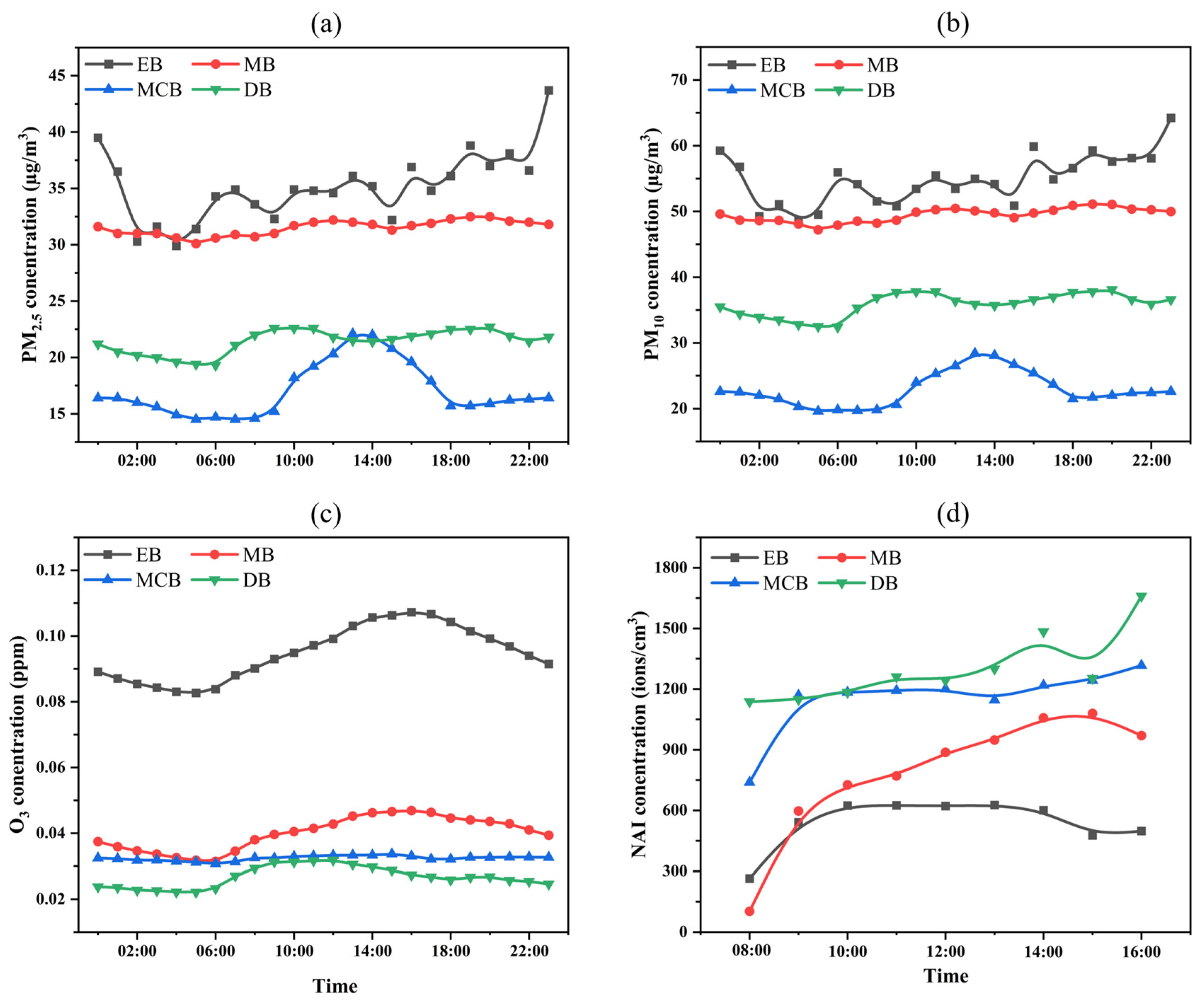
3.1. The Changing Trends of Concentrations of Air Pollutants and NAI

The results of this study show significant monthly fluctuations in the concentrations of air pollutants and NAI across the four forest types. During the summer, the peak concentrations of PM2.5, PM10, and O3 were observed in June for all four forest types, with the lowest concentrations occurring in July. The overall trend in monthly average concentrations showed an initial decrease followed by an increase. From June to August, PM2.5 and PM10 concentrations in EB and MB were higher than those in MCB and DB. In July, the air PM2.5 concentrations for the four forest types, in ascending order, were DB (19.2 μg/m3), MCB (19.4 μg/m3), MB (25.2 μg/m3), and EB (27.3 μg/m3) (Figure 2a). The PM10 concentrations, in ascending order, were MCB (24.5 μg/m3), DB (28.4 μg/m3), MB (36.8 μg/m3), and EB (38.7 μg/m3) (Figure 2b). The O3 concentration in EB was significantly higher than in MCB and DB during the summer (p < 0.05), with EB having O3 concentrations 1.2 to 4 times greater than those of the other three forest types (Figure 2c). The daily average concentration of NAI in different forest types is as follows: DB (1287 ions/cm3) > MCB (1187 ions/cm3) > MB (896 ions/cm3) > EB (584 ions/cm3) (Figure 2d).
The diurnal variations in PM2.5 concentration, PM10 concentration, O3 concentration, and NAI concentration within the four forest types are illustrated in Figure 3. The lowest points for both PM2.5 and PM10 concentrations in all four forest types occurred around 5:00 a.m. The peak concentrations for PM2.5 and PM10, except for EB (which occurred at 11:00 p.m.), were observed during the midday period (10:00 a.m. to 2:00 p.m.). The minimum O3 concentrations for all four forest types were found around 6:00 a.m., while the peak O3 concentrations were observed around 4:00 p.m., except for DB, where the peak occurred at 11:00 a.m. The NAI concentration in MB, MCB, and DB all exhibited a similar gradual upward trend. Only in EB did the NAI concentration peak at 10:00 a.m. and then tend to stabilize. The lowest NAI concentrations for all four forest types were observed at 8:00 a.m. Except for EB, the NAI peak concentrations in the other three forest types occurred between 2:00 p.m. and 4:00 p.m.

3.2. The Relationship Between Forest Structure and Air Quality

Multiple regression analyses were conducted for summer stand structure parameters with PM2.5, PM10, O3, and NAI to determine the relationship between air quality factors and forest stand structure parameters. In these analyses, PM2.5, PM10, O3, and NAI served as dependent variables, and the forest stand structure parameters (TH, DBH, SD, SHD, CHL, CD, SDS, SDH, SWS, and SWH) from the eight sample plots served as independent variables. Stepwise regression analysis was used to fit a model of summer stand structure and air quality, with results presented in Table 4. In the context of summer forest structural parameters, both SD and SWH significantly influence particulate matter concentrations. Specifically, SD exhibits a significant positive correlation with PM2.5 concentrations, whereas SWH shows a significant negative correlation. A similar pattern is observed for PM10, which is also significantly modulated by SD and SWH. TH has a significant negative correlation with O3 concentrations, whereas CD displays a significant positive correlation. In the forest stand structure, NAI was positively associated with TH (p = 0.059) and negatively associated with DBH (p = 0.065). Although the significance levels of both variables slightly exceeded the 0.05 threshold, the model explained 40.5% of the variance in NAI, suggesting that the combination of these variables has an important influence on NAI.

3.3. The Impact of Environmental Factors on Air Quality

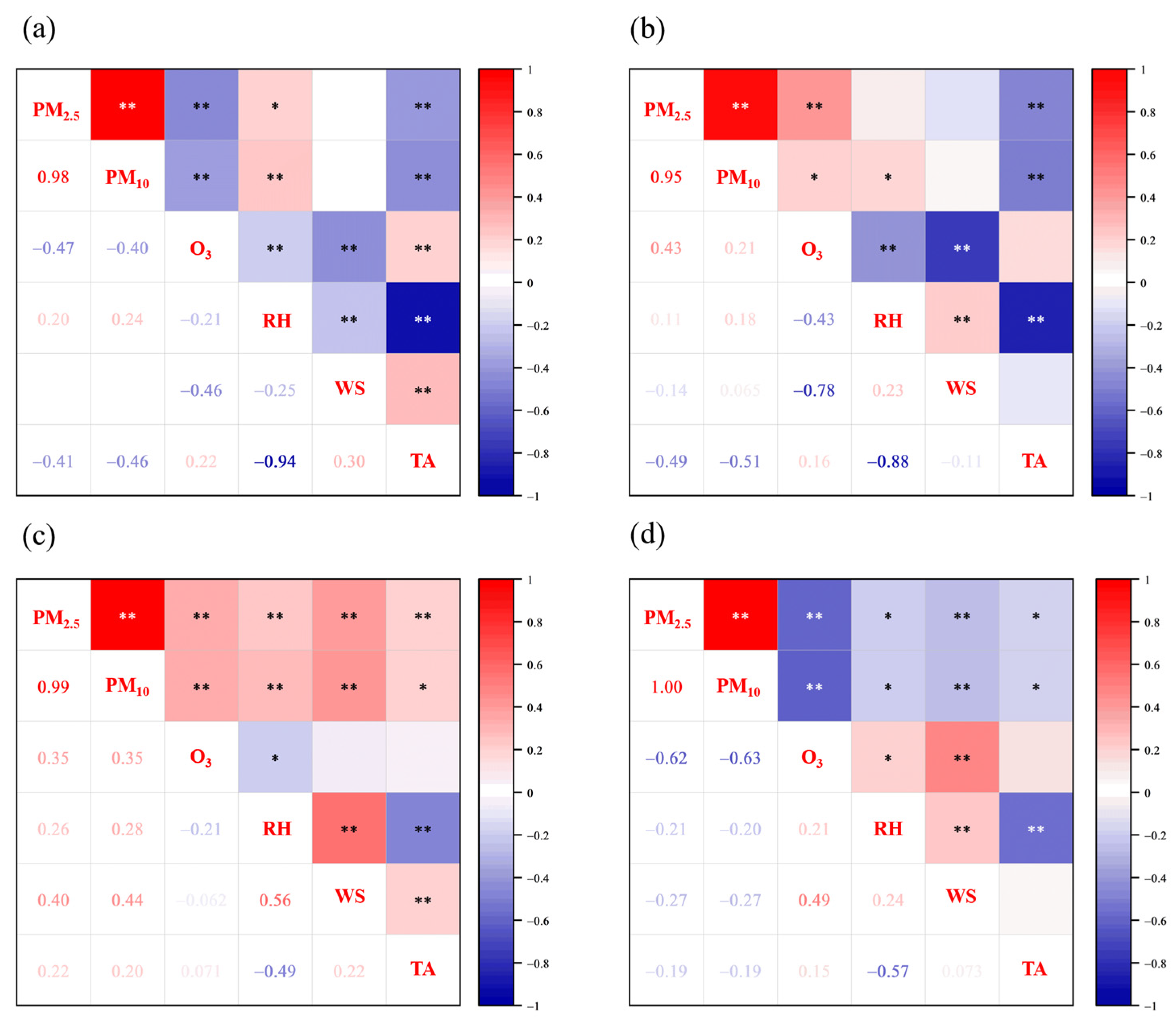
3.3.1. The Impact of Environmental Factors on Air Pollutants

This paper analyzed the correlations between RH, TA, WS, PM2.5, PM10, and O3, with the results shown in Figure 4. A significant negative correlation (p < 0.05) was found between RH and PM2.5 concentration and PM10 concentration in DB, while a significant positive correlation was found in EB, MB, and MCB. Except for MCB, which showed a significant positive correlation (p < 0.05) between TA and PM2.5 concentration and PM10 concentration, the other three forest types showed a significant negative correlation. The O3 concentration in all four forest types was negatively influenced by RH and WS and positively correlated with changes in TA.
Multiple linear regression analyses were conducted using these three environmental factors (RH, TA, and WS) with PM2.5, PM10, and O3, respectively. Table 5 presents the results of the multiple linear regression equations. From the multiple linear regression equations for PM2.5 concentration, the R2 values, ranked from highest to lowest, were MB (0.745), EB (0.451), MCB (0.256), and DB (0.165). Except for MCB, the PM2.5 concentrations of the other forest types were significantly negatively influenced by RH and TA (p < 0.01). The PM2.5 concentration in MCB was significantly negatively influenced by RH and positively influenced by WS (p < 0.01). Additionally, the PM2.5 concentration in EB was also positively influenced by WS (p < 0.05). For the multiple linear regression equations of PM10 concentration in each forest type, the R2 values, ranked from highest to lowest, were MB (0.716), EB (0.601), MCB (0.292), and DB (0.175). The meteorological factors influencing the PM10 concentration of each forest type were consistent with those influencing the PM2.5 concentration. In the regression equations for O3 concentration, the R2 values, ranked from highest to lowest, were MB (0.670), EB (0.536), MCB (0.167), and DB (0.129). The O3 concentration in EB was significantly positively influenced by RH and TA and significantly negatively influenced by WS (p < 0.001). The O3 concentration in MB was significantly negatively influenced by RH, TA, and WS (p < 0.001). The O3 concentration in MCB was significantly negatively influenced by RH and TA and significantly positively influenced by WS (p < 0.001). The O3 concentration in DB was only significantly positively influenced by WS (p < 0.001).

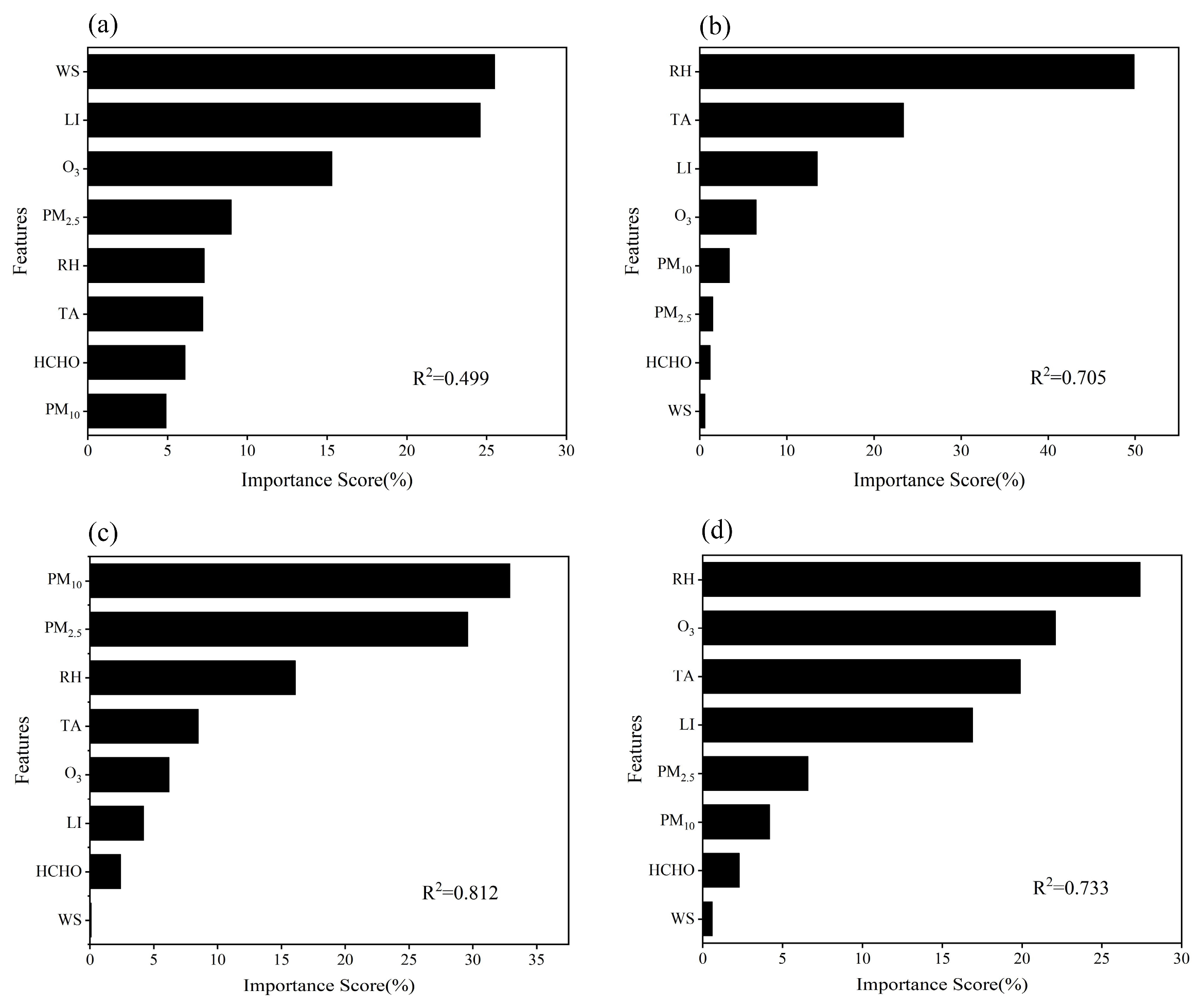
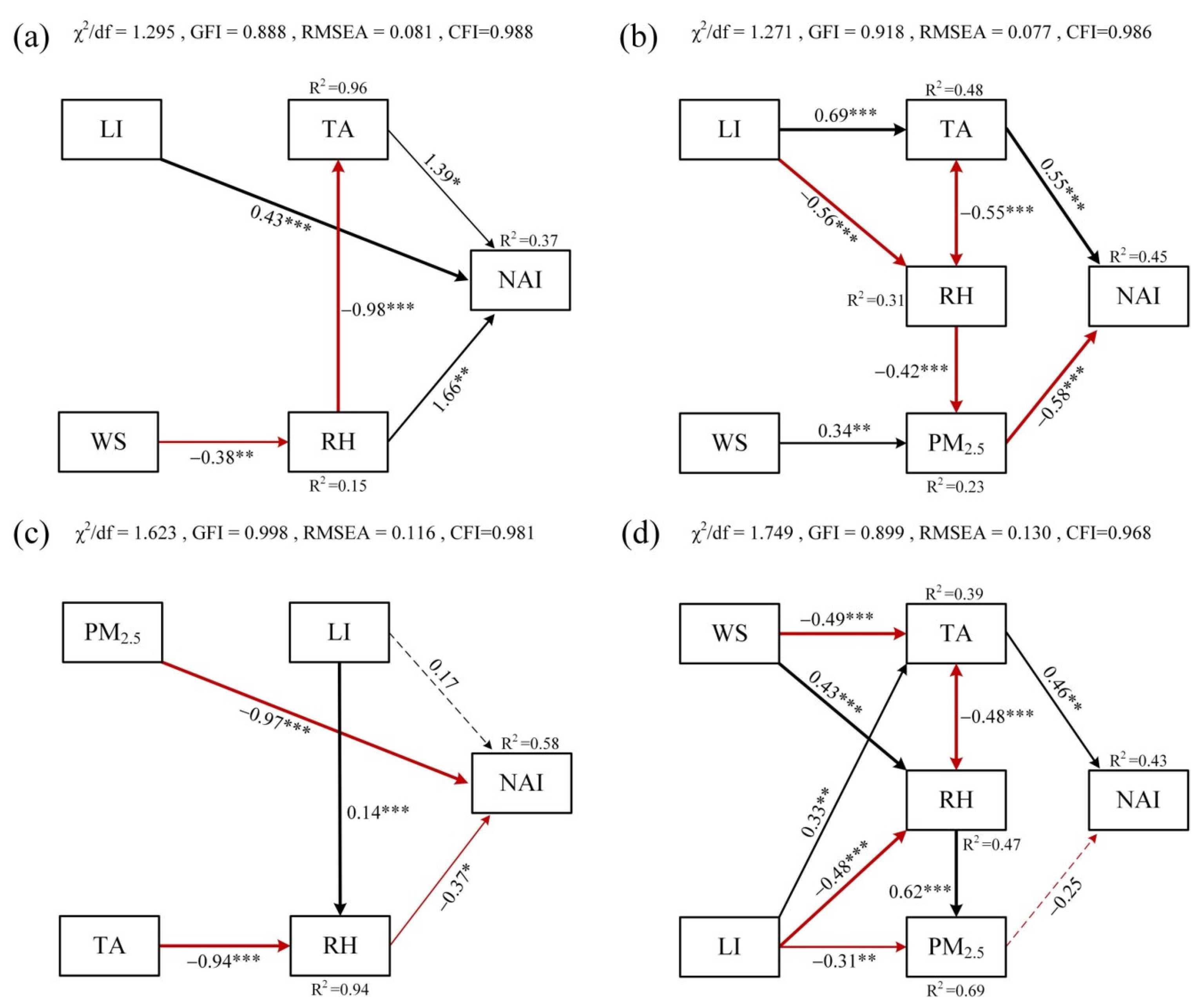
3.3.2. The Impact of Environmental Factors on NAI

This study analyzed the correlations between environmental factors and NAI concentration and their contributions to NAI concentration. Due to the numerous influencing factors, a random forest model and path analysis were employed. Figure 5 displays the correlations between environmental factors and NAI concentration for each forest type. The random forest model also analyzed eight factors (RH, TA, WS, LI, PM2.5, PM10, O3, and HCHO) and ranked their importance to NAI concentration from highest to lowest. The main factors influencing NAI concentration in EB, from highest to lowest, were WS, LI, O3, PM2.5, RH, and TA (Figure 6a). For MB, the main factors were RH, TA, LI, and O3 (Figure 6b). For MCB, the main factors were PM10, PM2.5, RH, TA, and O3 (Figure 6c). For DB, the main factors were RH, O3, TA, LI, and PM2.5 (Figure 6d). Path models were used to further examine the degree and way variables influence NAI concentration.
The path model analysis examined the direct and indirect effects of predictor variables on NAI concentration. TA, WS, LI, and RH had the greatest influence on NAI concentration in EB, with standardized total effects of 1.39, −0.63, 0.43, and 0.29, respectively (Figure 7a). TA and WS played a significant role in NAI variations in EB. In addition to a significant positive direct effect of TA on NAI (p < 0.05), WS altered NAI concentration indirectly by influencing RH. The model showed that the variables above could explain 37% of the variation in NAI concentration in EB. PM2.5, TA, RH, WS, and LI had the greatest influence on NAI concentration in MB, with standardized total effects of −0.58, 0.42, 0.25, −0.20, and 0.15, respectively (Figure 7b). PM2.5 and TA had a significant impact on NAI concentration in MB. PM2.5 directly and significantly negatively influenced NAI concentration (p < 0.001). Besides having a direct and highly significant positive influence on NAI concentration (p < 0.001), TA also indirectly affected NAI concentration changes through its interaction with RH. The model showed that the variables above could explain 45% of the NAI concentration variation in MB. PM2.5, RH, TA, and LI had the greatest influence on NAI concentration in MCB, with standardized total effects of −0.97, −0.37, 0.35, and 0.12, respectively (Figure 7c). PM2.5 directly and significantly negatively influenced NAI concentration in MCB (p < 0.001). The model showed that the abovementioned variables could explain 58% of the NAI concentration variation in MCB. TA, WS, LI, RH, and PM2.5 had the greatest influence on NAI concentration in DB, with standardized total effects of 0.64, −0.47, 0.47, −0.38, and −0.25, respectively (Figure 7d). TA directly and significantly positively affected NAI concentration (p < 0.01) and indirectly affected NAI concentration changes through its interaction with RH. The model showed that the variables above could explain 43% of the NAI concentration variation in DB.

4. Discussion

4.1. Differences in Air Quality Among Different Forest Types

4.1.1. PM Concentration

This study revealed significant differences in air quality among the four forest types (EB, MB, MCB, and DB) during the growing season. Congzhe Liu et al. [24] found that mixed coniferous and broadleaf forests had the strongest reduction capacity for PM2.5 and PM10, followed by deciduous broadleaf forests, and the weakest was evergreen broadleaf forests. This finding aligns with the results of the present study. The dominant tree species in both mixed coniferous and broadleaf forests and deciduous broadleaf forests, with a remarkable capacity for PM reduction, are Cryptomeria fortunei, Ginkgo biloba, Bischofia javanica, Quercus acutissima, and Liquidambar formosana. The leaf surfaces of these plants are mostly rough, sticky, or pubescent, which increases the contact area and adsorption capacity for PM, thus allowing them to better capture airborne particulate matter.

4.1.2. Ozone Concentration

Our findings showed that EB exhibited the highest ozone concentration, significantly exceeding the levels in the other three forest types, which parallels the research of Li Shaoning et al. [25] Li’s work showed that evergreen broadleaf forests in Nanhai Zi Park had higher ozone concentrations than mixed coniferous and broadleaf forests. This phenomenon is often attributed to the higher temperatures and elevated levels of biogenic volatile organic compounds (BVOCs) found within broadleaf forests, which subsequently promote the accumulation of O3 within the forest environment [26,27]. Numerous studies have established a strong link between BVOC release and air quality, particularly ozone levels, with large quantities of BVOC release leading to a 20%–49% surge in O3 concentrations [16,28,29]. The efficiency of plant BVOC release and the capacity to remove O3 are primarily determined by community makeup, stand structure, and environmental elements influencing tree growth [30].

4.1.3. NAI Concentration

This study observed higher concentrations of NAI in deciduous broadleaf forests and mixed coniferous and broadleaf forests, consistent with the conclusions of most prior studies. Deng Cheng et al. [21] reported that the NAI concentration in mixed coniferous and broadleaf forests was higher than that in evergreen broadleaf forests. However, some studies do not support our findings. Wang Yihao et al. [31], in their study of forest stands in Chongqing, found that the NAI concentration ranking during summer from highest to lowest was deciduous broadleaf forests, evergreen broadleaf forests, moso bamboo forests, and mixed coniferous and broadleaf forests. Through comparison, we believe that the higher NAI concentration in MCB in our study is related to the complex spatial structure of vegetation within the forest, rich plant diversity, and taller trees. Furthermore, our study showed that the NAI concentration in EB was the lowest among the four forest types, even significantly lower than the NAI concentration in MB, which contradicts some research results. Aibo Li et al. [19], in their study of subtropical typical forests, found that the NAI concentration in evergreen broadleaf mixed forests was the highest, higher than that in moso bamboo and coniferous forests. This discrepancy may be due to differences in tree species composition, stand structure, and the microclimate of the forest environment [32]. In our study, the stand density of EB was only one-sixth that of MB, and the average tree height of EB was the lowest among the four forest types. Simultaneously, the herbaceous plant coverage, Shannon–Wiener index, and Simpson index were significantly lower than those of other forest types, which may be the main reasons limiting the NAI release capacity.

4.2. Factors Affecting Air Quality in Different Forest Types

4.2.1. The Impact of Plant Groups on Air Quality

Vegetation is one of the most important factors in reducing regional PM concentrations [9,33]. Numerous studies investigating the impact of forest vegetation on ambient PM concentrations have shown that different vegetation compositions can reduce airborne PM concentrations through various pathways, including ground cover, pollutant adsorption, and influencing meteorological factors [34,35,36,37]. Different vegetation types and the single-leaf characteristics of tree species within a community can significantly affect PM concentrations in a specific area [38]. Under similar environmental conditions, leaves with sticky or rough surfaces can capture more particulate matter than smooth leaves [12,39]. The adsorption of particulate matter by plants mainly occurs during the growing season, and leaf quantity and shape are also major factors affecting air quality. Smaller leaves and complex leaf shapes have a greater capacity for PM retention [40]. For example, the leaf surface of Cryptomeria fortunei has deep, striated grooves and irregularly arranged nodular protrusions, and these microstructures increase the surface area of the leaves, enabling them to better adsorb PM. In areas with abundant vegetation, the BVOCs released by vegetation can chemically react with ozone. During this process, the released electrons combine with oxygen ions to form negative oxygen ions, which can improve local air quality.

4.2.2. The Impact of Forest Structure on Air Quality

The complex spatial structure of vegetation reduces airflow velocity and hinders the diffusion of PM and NAI to the outside environment, thereby leading to a decrease in PM concentration and a continuous increase in NAI concentration within the forest. Investigations into stand-level and vertical structures have confirmed that dense vegetation has a stable mitigating effect on PM2.5 and can create a relatively clean air environment, even under severe PM pollution [41,42]. Notably, single-layered stands exhibit unique differences in their effectiveness at mitigating PM2.5. Due to their relatively simple structure and the lack of multi-layered vegetation interception and regulation mechanisms, PM2.5 demonstrates two distinctly different patterns of change within single-layered stand areas: either rapid dispersion or rapid accumulation [43]. Stands with complex vertical structures of trees, shrubs, and herbs can effectively slow down airflow and better remove airborne particulate matter [44,45], ensuring higher NAI concentrations within the forest. Among the many factors influencing NAI concentration within a forest, shrub density and tree height diversity index play particularly prominent roles [19]. Shrub density influences the spatial layout and airflow patterns within a stand, while the tree height diversity index reflects the complexity and diversity of the stand in the vertical dimension. Together, these two factors significantly impact NAI concentration within the forest.
Among the factors measuring the air purification capacity of trees, diameter at breast height is crucial. Trees with larger DBH tend to have superior air purification abilities. As demonstrated by Chunyang Zhu et al. [15] in their 2019 research, the reduction in PM concentration is closely related to DBH and leaf area index (LAI). Plant communities with larger DBH have a significantly stronger dust accumulation capacity and can effectively adsorb and reduce the amount of PM in the air [46]. This is because trees with larger DBH also have a larger leaf area index. The rich microstructure and large total surface area of these trees greatly enhance their ability to adsorb air pollutants.
In addition to tree DBH, vegetation cover also reflects a forest stand’s ability to improve air quality. Related studies have found that higher tree cover has a significant positive effect on air quality compared to open areas. For example, Vesa Yli-Pelkone [47] demonstrated that higher tree density can significantly reduce ozone concentration. This phenomenon is particularly evident in urban environments. According to Kun Liu’s 2024 study [48], the PM2.5 and O3 concentrations in urban forest areas were 34.3% and 12.6% lower, respectively, than in urban areas from 10:00 to 15:00. Simultaneously, areas with high vegetation cover also have excellent regulatory capacity for forest microclimate. Through physiological and physical processes such as transpiration and the absorption and reflection of light and heat, vegetation effectively regulates meteorological factors such as temperature and humidity within the forest, thereby indirectly affecting pollutant concentrations and the rate at which vegetation releases NAI.

4.2.3. Impact of Environmental Factors on Air Quality

In this study, the correlation between TA and PM concentration was negative, and the results of the multiple regression equations showed that PM concentration decreased with increasing TA. Increased temperature may enhance local air convection within the forest, carrying PM from inside the forest to the outside. At the same time, increased temperature also promotes plant metabolic activity, leading to an enhanced capacity of plants to adsorb PM [49]. There is a close relationship between temperature and humidity in summer forest environments; increased temperature is usually accompanied by increased humidity, which makes PM more easily adsorb water vapor, increasing their particle size and thus accelerating their deposition. Alternatively, a decrease in air temperature may lead to temperature inversion [50]. The occurrence of temperature inversion reduces surface wind speed, causing pollutants in the air to easily accumulate and be difficult to disperse, leading to an increase in PM2.5 concentration. The four forest types showed two distinctly different results in the relationship between TA and NAI concentration in this study. TA was negatively correlated with NAI concentration in EB and MCB, while TA was positively correlated with NAI in MB and DB. The reason for this may be that increased TA accelerates the movement of charged particles within the forest and also accelerates photosynthesis in the vegetation within MB and DB, further promoting NAI production by accelerating the release of oxygen [51]. EB and MCB, with their lower stand densities, may have high-temperature, high-humidity environments that are not conducive to NAI production. Some studies have reported similar results; Aibo Li et al. [52] found that the feedback effect of NAI concentration on TA gradually decreased within a certain range.
Vegetation influences RH in the air through its own transpiration [53]; in this study, RH had a significant impact on PM concentration within the forest, but the relationship between RH and PM concentration was not a simple linear correlation. The results of the multiple regression equations showed that PM concentration decreased with increasing RH, which is consistent with the research results of Ryu et al. [11]. Ryu confirmed in their report that the increased RH due to plant transpiration is critical for reducing PM. The effect of plant communities on particulate matter in the air is very complex. Generally, when the relative humidity of the air in a forest increases, the PM will absorb water vapor from the air, causing the particle size to increase, a process known as hygroscopic growth [54]. Particles with larger sizes have a slower settling velocity in the air, which extends their residence time in the forest air. Therefore, over a certain period, PM concentration may appear to increase with increasing RH [55]. When the relative humidity reaches a certain level, the high humidity increases the stickiness of the plant leaf surface, further improving its efficiency in removing PM [56]. In our study of the relationship between RH and NAI concentration, we found results similar to those for TA. RH was positively correlated with NAI concentration in EB and MCB, while RH was negatively correlated with NAI in MB and DB. Related studies have shown that there is a certain fitting relationship between RH and NAI concentration. As RH increases, NAI concentration initially decreases, then increases, and then finally decreases [57]. Under high humidity conditions, as RH continues to increase, NAI concentration will gradually decrease, possibly because NAI loses its biological effect at higher humidity [58].
Many scholars have studied the relationship between WS, PM, and NAI, reaching different and even contradictory results. Yanan Wu et al. [59] proposed that the collection rate of PM2.5 and PM10 is positively correlated with wind speed, but other scholars have found that PM concentration is not significantly correlated with wind speed [60], which may be related to the aerosols generated by mechanical friction caused by wind. In our study, there was no clear pattern in the relationship between WS and PM within the four forest types, and WS was negatively correlated with NAI concentration, which is consistent with the views of other scholars [20]. Some scholars have proposed that a large amount of NAI is generated through air friction when wind speed is between 3 and 10 m/s. However, studies have found that the average wind speed in forests is much lower than this value, so NAI generation through air friction does not fit the actual situation of the sample plots in this study. Therefore, we believe that the impact of wind speed within the forest on air quality is mainly through wind at a given moment blowing particulate matter and NAI past the monitoring equipment, which leads to no clear correlation in the air quality data collected by the instrument [18]. I suggest further exploring the influence of wind speed within the forest through controlled variable experiments.

4.3. Suggestions on Selecting Healthy Forest Stands and the Timing of Healthcare

Reasonable forest stand selection and time planning are crucial for achieving forest health benefits. Our study shows that NAI concentrations in the four subtropical forest stands during the summer can meet human therapy requirements. We recommend conducting health and fitness activities such as sitting meditation, mindfulness meditation, and Tai Chi in MCB and DB forests. These two forest types have lower PM and ozone concentrations, and the average NAI concentrations within them exceed the fresh air threshold defined by the World Health Organization [61], indicating better air quality. Therefore, longer-duration health activities are more suitable for these two stands. Additionally, the timing of forest activities should be arranged in the afternoon (14:00–16:00), when NAI concentrations within the forest are at their highest. This recommendation is consistent with the views of Aibo Li et al. [19], who suggest that outdoor leisure and forest therapy activities are most beneficial in the afternoon (15:00–17:00) or early morning (5:00–7:00).

5. Conclusions

In this study, we conducted three months of continuous monitoring of four forest types, revealing the spatiotemporal dynamics of summer air quality and the factors influencing its concentration. The following conclusions were drawn. Firstly, the forest air quality is at its best in July during the summer season, and there are significant differences in air quality among different forest stands. Among these forest types, mixed coniferous and broadleaf forests and deciduous broadleaf forests have the lowest PM concentrations and O3 concentrations. Secondly, the troughs of PM concentrations occur in the early morning (4:00–6:00), while the troughs of O3 concentrations occur in the early morning (4:00–6:00) and in the evening (18:00). Thirdly, NAI concentrations were highest in deciduous broadleaf forests, followed by mixed coniferous and broadleaf forests, moso bamboo forests, and evergreen broadleaf forests, with NAI concentrations peaking between 14:00 and 16:00. Fourthly, PM concentrations in forest air were primarily influenced by SD and SWH (p < 0.05); ozone concentrations were significantly affected by TH and CD (p < 0.05); and NAI concentrations were primarily related to TH and DBH. Finally, air particulate matter concentrations were negatively affected by TA and RH (p < 0.01), ozone concentrations were negatively influenced by RH and WS and were positively influenced by TA. NAI concentration was negatively impacted by WS and positively impacted by LI. Meanwhile, TA has a direct and significant positive effect on the NAI concentration (p < 0.01), and RH indirectly influences the changes in NAI concentration through its interaction with TA.
By analyzing the stand structure and environmental factors of four typical subtropical forests, the results of this study have significant implications for urban green space planning, forest protection, and public health. In urban green space planning, tree species with strong purification ability can be planted in high pollution areas based on the relationship between tree species and air quality, and green space layout can be designed referring to forest structure. In terms of forest protection, we protect and restore tree species that are crucial for maintaining air quality and carry out related afforestation projects to maintain the integrity of forest ecosystems. In the field of public health, based on the benefits of forests for health, activities such as forest bathing and hiking are promoted to help improve respiratory health.
This study was conducted in specific regions and forest types, and due to the relatively small number of sample plots, there are certain limitations in generalizing the results to other regions. The data collection for this study was focused on summer, which inevitably brought seasonal constraints. The activities of forest ecosystems vary significantly in different seasons; subsequent research can collect and analyze data from different seasons throughout the year to further improve. Simultaneously install fixed negative oxygen ion monitoring equipment to collect long-term negative oxygen ion data. Among the factors affecting air quality, the negative impact of human factors was not taken into account. Future research should aim to expand the range of forest types and extend the monitoring time to capture seasonal changes in air quality. Other variables such as human activities and soil conditions should be considered and included in the analysis. Researchers should simultaneously consider interdisciplinary collaboration, collaborate with medical and health experts, and participate in evaluating the physiological benefits of different forest types.

Author Contributions

Z.J., data curation, formal analysis, and writing—original draft; R.Z., formal analysis and validation; J.J., writing—review and editing; C.P., writing—review and editing; Z.C., investigation; Y.H., investigation; Y.Z., resources and project administration; G.Z., conceptualization, funding acquisition, supervision, and writing—review and editing. All authors have read and agreed to the published version of the manuscript.

Funding

This research was funded by the Key Research and Development Program of Zhejiang Province (Grant Nos. 2021C02005 and 2022C03039).

Data Availability Statement

The original contributions presented in this study are included in the article. Further inquiries can be directed to the corresponding author.

Conflicts of Interest

The authors declare no conflicts of interest.

Abbreviations

The following abbreviations are used in this manuscript:
PMparticulate matter
PM2.5fine particulate matter
PM10inhalable particulate matter
O3ozone
NAInegative air ion
BVOCsbiogenic volatile organic compounds
EBevergreen broad-leaved forests
MBmoso bamboo plantations
MCBmixed coniferous and broad-leaved forests
DBdeciduous broad-leaved forests
THtree height
DBHdiameter at breast height
SDstand density
SHDshrub density
CHLcoverage of herb layer
CDcanopy density
SDSSimpson diversity index of shrubs layer
SDHSimpson diversity index of herbaceous Layer
SWSShannon–Wiener index of shrub layer
SWHShannon–Wiener index of herbaceous Layer
TAair temperature
RHrelative humidity
WSwind speed
LIlight intensity
CO2carbon dioxide

References

  1. Liang, L.; Wang, Z.; Li, J. The effect of urbanization on environmental pollution in rapidly developing urban agglomerations. J. Clean. Prod. 2019, 237, 117649. [Google Scholar] [CrossRef]
  2. World Health Organization. WHO Global Air Quality Guidelines: Particulate Matter (PM2.5 and PM10), Ozone, Nitrogen Dioxide, Sulfur Dioxide and Carbon Monoxide; World Health Organization: Geneva, Switzerland, 2021. [Google Scholar]
  3. Reiter, R. Part B Frequency distribution of positive and negative small ion concentrations, based on many years’ recordings at two mountain stations located at 740 and 1780 m ASL. Int. J. Biometeorol. 1985, 29, 223–231. [Google Scholar] [CrossRef]
  4. Lu, X.; Lin, C.; Li, W.; Chen, Y.; Huang, Y.; Fung, J.C.; Lau, A.K. Analysis of the adverse health effects of PM2.5 from 2001 to 2017 in China and the role of urbanization in aggravating the health burden. Sci. Total Environ. 2019, 652, 683–695. [Google Scholar] [CrossRef]
  5. Mudway, I.; Kelly, F. Ozone and the lung: A sensitive issue. Mol. Asp. Med. 2000, 21, 1–48. [Google Scholar] [CrossRef] [PubMed]
  6. Krueger, A.P.; Reed, E.J. Biological Impact of Small Air Ions: Despite a history of contention, there is evidence that small air ions can affect life processes. Science 1976, 193, 1209–1213. [Google Scholar] [CrossRef]
  7. Chen, L.; Liu, C.; Zhang, L.; Zou, R.; Zhang, Z. Variation in tree species ability to capture and retain airborne fine particulate matter (PM2.5). Sci. Rep. 2017, 7, 3206. [Google Scholar] [CrossRef]
  8. Chen, L.; Sun, B.; Tan, G.; Li, Z.; Chen, Y.; Huang, Y.; Liao, S. Plant species structure and diversity of plant communities in Guangzhou parks. Ecol. Sci. 2015, 34, 38–44. [Google Scholar] [CrossRef]
  9. Chen, L.; Liu, C.; Zou, R.; Yang, M.; Zhang, Z. Experimental examination of effectiveness of vegetation as bio-filter of particulate matters in the urban environment. Environ. Pollut. 2016, 208, 198–208. [Google Scholar] [CrossRef]
  10. Cai, L.; Shi, G.; Zhang, J.; Du, L.; Ni, X.; Hu, Y.; Pang, D.; Meng, J. Empirical analysis of the influence mechanism of vegetation and environment on negative air ion in warm temperate forest ecosystems. Environ. Pollut. 2024, 363, 125273. [Google Scholar] [CrossRef]
  11. Ryu, J.; Kim, J.J.; Byeon, H.; Go, T.; Lee, S.J. Removal of fine particulate matter (PM2.5) via atmospheric humidity caused by evapotranspiration. Environ. Pollut. 2019, 245, 253–259. [Google Scholar] [CrossRef]
  12. Sæbø, A.; Popek, R.; Nawrot, B.; Hanslin, H.; Gawronska, H.; Gawronski, S. Plant species differences in particulate matter accumulation on leaf surfaces. Sci. Total Environ. 2012, 427, 347–354. [Google Scholar] [CrossRef] [PubMed]
  13. Hu, Y.; Zhao, P.; Niu, J.; Sun, Z.; Zhu, L.; Ni, G. Canopy stomatal uptake of NOX, SO2 and O3 by mature urban plantations based on sap flow measurement. Atmos. Environ. 2016, 125, 165–177. [Google Scholar] [CrossRef]
  14. Jeong, N.-R.; Han, S.-W.; Kim, J.-H. Evaluation of vegetation configuration models for managing particulate matter along the urban street environment. Forests 2022, 13, 46. [Google Scholar] [CrossRef]
  15. Zhu, C.; Przybysz, A.; Chen, Y.; Guo, H.; Chen, Y.; Zeng, Y. Effect of spatial heterogeneity of plant communities on air PM10 and PM2.5 in an urban forest park in Wuhan, China. Urban For. Urban Green. 2019, 46, 126487. [Google Scholar] [CrossRef]
  16. Liu, Y.; Li, L.; An, J.; Huang, L.; Yan, R.; Huang, C.; Wang, H.; Wang, Q.; Wang, M.; Zhang, W. Estimation of biogenic VOC emissions and its impact on ozone formation over the Yangtze River Delta region, China. Atmos. Environ. 2018, 186, 113–128. [Google Scholar] [CrossRef]
  17. Liu, S.; Huang, Q.; Wu, Y.; Song, Y.; Dong, W.; Chu, M.; Yang, D.; Zhang, X.; Zhang, J.; Chen, C. Metabolic linkages between indoor negative air ions, particulate matter and cardiorespiratory function: A randomized, double-blind crossover study among children. Environ. Int. 2020, 138, 105663. [Google Scholar] [CrossRef]
  18. Wang, H.; Wang, B.; Niu, X.; Song, Q.; Li, M.; Luo, Y.; Liang, L.; Du, P.; Peng, W. Study on the change of negative air ion concentration and its influencing factors at different spatio-temporal scales. Glob. Ecol. Conserv. 2020, 23, e01008. [Google Scholar] [CrossRef]
  19. Li, A.; Li, Q.; Yang, Y.; Hu, Y.; Xiao, S.; Li, Z.; Zhou, B. Stand structure and environment jointly determine negative air ion concentrations in forests: Evidence from concurrent on-site monitoring in four typical subtropical forests during the growing season. Environ. Exp. Bot. 2024, 220, 105684. [Google Scholar] [CrossRef]
  20. Kalivitis, N.; Stavroulas, I.; Bougiatioti, A.; Kouvarakis, G.; Gagné, S.; Manninen, H.; Kulmala, M.; Mihalopoulos, N. Night-time enhanced atmospheric ion concentrations in the marine boundary layer. Atmos. Chem. Phys. 2012, 12, 3627–3638. [Google Scholar] [CrossRef]
  21. Deng, C.; Zhang, S.; Lu, Y. Research on the Monitoring and Evaluation of Forest Function in Air Environmental Quality Improvement. Ecol. Environ. Sci. 2015, 24, 84–89. [Google Scholar] [CrossRef]
  22. Zhu, S.; Wang, R.; Wang, Q.; Lei, T.; Cui, G. Coniferous and broad-leaved mixed forest has the optimal forest therapy environment among stand types in Xinjiang. Ecol. Indic. 2024, 169, 112950. [Google Scholar] [CrossRef]
  23. Shi, G.-Y.; Zhou, Y.; Sang, Y.-Q.; Huang, H.; Zhang, J.-S.; Meng, P.; Cai, L.-L. Modeling the response of negative air ions to environmental factors using multiple linear regression and random forest. Ecol. Inform. 2021, 66, 101464. [Google Scholar] [CrossRef]
  24. Liu, C.; Dai, A.; Ji, Y.; Sheng, Q.; Zhu, Z. Effect of different plant communities on fine particle removal in an urban road greenbelt and its key factors in Nanjing, China. Sustainability 2022, 15, 156. [Google Scholar] [CrossRef]
  25. Li, S.; Li, A.; Shi, C.; Zhao, N.; Xu, X.; Zheng, L.; Guo, J.; Lu, S. Interactive Response Mechanism of Different Urban Forest Stands to Negative Air Ion and Ozone Concentration. J. Southwest For. Univ. (Nat. Sci.) 2023, 43, 74–80. [Google Scholar]
  26. Aydin, Y.M.; Yaman, B.; Koca, H.; Dasdemir, O.; Kara, M.; Altiok, H.; Dumanoglu, Y.; Bayram, A.; Tolunay, D.; Odabasi, M. Biogenic volatile organic compound (BVOC) emissions from forested areas in Turkey: Determination of specific emission rates for thirty-one tree species. Sci. Total Environ. 2014, 490, 239–253. [Google Scholar] [CrossRef]
  27. Guidolotti, G.; Pallozzi, E.; Gavrichkova, O.; Scartazza, A.; Mattioni, M.; Loreto, F.; Calfapietra, C. Emission of constitutive isoprene, induced monoterpenes, and other volatiles under high temperatures in Eucalyptus camaldulensis: A 13C labelling study. Plant Cell Environ. 2019, 42, 1929–1938. [Google Scholar] [CrossRef]
  28. Wu, K.; Yang, X.; Chen, D.; Gu, S.; Lu, Y.; Jiang, Q.; Wang, K.; Ou, Y.; Qian, Y.; Shao, P. Estimation of biogenic VOC emissions and their corresponding impact on ozone and secondary organic aerosol formation in China. Atmos. Res. 2020, 231, 104656. [Google Scholar] [CrossRef]
  29. Li, N.; He, Q.; Greenberg, J.; Guenther, A.; Li, J.; Cao, J.; Wang, J.; Liao, H.; Wang, Q.; Zhang, Q. Impacts of biogenic and anthropogenic emissions on summertime ozone formation in the Guanzhong Basin, China. Atmos. Chem. Phys. 2018, 18, 7489–7507. [Google Scholar] [CrossRef]
  30. Fitzky, A.C.; Sandén, H.; Karl, T.; Fares, S.; Calfapietra, C.; Grote, R.; Saunier, A.; Rewald, B. The interplay between ozone and urban vegetation—BVOC emissions, ozone deposition, and tree ecophysiology. Front. For. Glob. Change 2019, 2, 50. [Google Scholar] [CrossRef]
  31. Wang, Y.; Liu, F.; Zhou, X.; Liu, X.; Li, L. Air Anions Content and Its Evaluation for Main Forest Types in Chongqing. J. Northeast. For. Univ. 2014, 42, 38–42. [Google Scholar] [CrossRef]
  32. Kousis, I.; Manni, M.; Pisello, A. Environmental mobile monitoring of urban microclimates: A review. Renew. Sustain. Energy Rev. 2022, 169, 112847. [Google Scholar] [CrossRef]
  33. Jeanjean, A.P.; Monks, P.S.; Leigh, R.J. Modelling the effectiveness of urban trees and grass on PM2.5 reduction via dispersion and deposition at a city scale. Atmos. Environ. 2016, 147, 1–10. [Google Scholar] [CrossRef]
  34. Popek, R.; Przybysz, A.; Gawrońska, H.; Klamkowski, K.; Gawroński, S.W. Impact of particulate matter accumulation on the photosynthetic apparatus of roadside woody plants growing in the urban conditions. Ecotoxicol. Environ. Saf. 2018, 163, 56–62. [Google Scholar] [CrossRef]
  35. Viippola, V.; Whitlow, T.H.; Zhao, W.; Yli-Pelkonen, V.; Mikola, J.; Pouyat, R.; Setälä, H. The effects of trees on air pollutant levels in peri-urban near-road environments. Urban For. Urban Green. 2018, 30, 62–71. [Google Scholar] [CrossRef]
  36. Yin, S.; Chen, D.; Zhang, X.; Yan, J. Review on the multi-scale interactions of urban forests and atmospheric particles: Affecting factors are scale-dependent among tree, stand and region. Urban For. Urban Green. 2022, 78, 127789. [Google Scholar] [CrossRef]
  37. Przybysz, A.; Nersisyan, G.; Gawroński, S.W. Removal of particulate matter and trace elements from ambient air by urban greenery in the winter season. Environ. Sci. Pollut. Res. 2019, 26, 473–482. [Google Scholar] [CrossRef] [PubMed]
  38. Shao, F.; Wang, L.; Sun, F.; Li, G.; Yu, L.; Wang, Y.; Zeng, X.; Yan, H.; Dong, L.; Bao, Z. Study on different particulate matter retention capacities of the leaf surfaces of eight common garden plants in Hangzhou, China. Sci. Total Environ. 2019, 652, 939–951. [Google Scholar] [CrossRef]
  39. Baraldi, R.; Neri, L.; Costa, F.; Facini, O.; Rapparini, F.; Carriero, G. Ecophysiological and micromorphological characterization of green roof vegetation for urban mitigation. Urban For. Urban Green. 2019, 37, 24–32. [Google Scholar] [CrossRef]
  40. Weerakkody, U.; Dover, J.W.; Mitchell, P.; Reiling, K. Evaluating the impact of individual leaf traits on atmospheric particulate matter accumulation using natural and synthetic leaves. Urban For. Urban Green. 2018, 30, 98–107. [Google Scholar] [CrossRef]
  41. Zhai, H.; Yao, J.; Wang, G.; Tang, X. Study of the effect of vegetation on reducing atmospheric pollution particles. Remote Sens. 2022, 14, 1255. [Google Scholar] [CrossRef]
  42. Janhäll, S. Review on urban vegetation and particle air pollution–Deposition and dispersion. Atmos. Environ. 2015, 105, 130–137. [Google Scholar] [CrossRef]
  43. Su, T.-H.; Lin, C.-S.; Lu, S.-Y.; Lin, J.-C.; Wang, H.-H.; Liu, C.-P. Effect of air quality improvement by urban parks on mitigating PM2.5 and its associated heavy metals: A mobile-monitoring field study. J. Environ. Manag. 2022, 323, 116283. [Google Scholar] [CrossRef] [PubMed]
  44. Abhijith, K.; Kumar, P.; Gallagher, J.; McNabola, A.; Baldauf, R.; Pilla, F.; Broderick, B.; Di Sabatino, S.; Pulvirenti, B. Air pollution abatement performances of green infrastructure in open road and built-up street canyon environments—A review. Atmos. Environ. 2017, 162, 71–86. [Google Scholar] [CrossRef]
  45. Deshmukh, P.; Isakov, V.; Venkatram, A.; Yang, B.; Zhang, K.M.; Logan, R.; Baldauf, R. The effects of roadside vegetation characteristics on local, near-road air quality. Air Qual. Atmos. Health 2019, 12, 259–270. [Google Scholar] [CrossRef]
  46. Kwak, M.J.; Lee, J.; Kim, H.; Park, S.; Lim, Y.; Kim, J.E.; Baek, S.G.; Seo, S.M.; Kim, K.N.; Woo, S.Y. The removal efficiencies of several temperate tree species at adsorbing airborne particulate matter in urban forests and roadsides. Forests 2019, 10, 960. [Google Scholar] [CrossRef]
  47. Yli-Pelkonen, V.; Scott, A.A.; Viippola, V.; Setälä, H. Trees in urban parks and forests reduce O3, but not NO2 concentrations in Baltimore, MD, USA. Atmos. Environ. 2017, 167, 73–80. [Google Scholar] [CrossRef]
  48. Liu, K.; Li, J.; Sun, L.; Yang, X.; Xu, C.; Yan, G. Impact of Urban Forest and Park on Air Quality and the Microclimate in Jinan, Northern China. Atmosphere 2024, 15, 426. [Google Scholar] [CrossRef]
  49. Ram, S.; Majumder, S.; Chaudhuri, P.; Chanda, S.; Santra, S.; Chakraborty, A.; Sudarshan, M. A review on air pollution monitoring and management using plants with special reference to foliar dust adsorption and physiological stress responses. Crit. Rev. Environ. Sci. Technol. 2015, 45, 2489–2522. [Google Scholar] [CrossRef]
  50. Schilperoort, B.; Coenders-Gerrits, M.; Rodríguez, C.J.; van Hooft, A.; van de Wiel, B.; Savenije, H. Detecting nighttime inversions in the interior of a Douglas fir canopy. Agric. For. Meteorol. 2022, 321, 108960. [Google Scholar] [CrossRef]
  51. Miao, S.; Zhang, X.; Han, Y.; Sun, W.; Liu, C.; Yin, S. Random forest algorithm for the relationship between negative air ions and environmental factors in an urban park. Atmosphere 2018, 9, 463. [Google Scholar] [CrossRef]
  52. Li, A.; Li, Q.; Zhou, B.; Ge, X.; Cao, Y. Temporal dynamics of negative air ion concentration and its relationship with environmental factors: Results from long-term on-site monitoring. Sci. Total Environ. 2022, 832, 155057. [Google Scholar] [CrossRef] [PubMed]
  53. Zhu, C.; Ji, P.; Li, S. Effects of urban green belts on the air temperature, humidity and air quality. J. Environ. Eng. Landsc. Manag. 2017, 25, 39–55. [Google Scholar] [CrossRef]
  54. Han, J.; Liu, X.; Chen, D.; Jiang, M. Influence of relative humidity on real-time measurements of particulate matter concentration via light scattering. J. Aerosol Sci. 2020, 139, 105462. [Google Scholar] [CrossRef]
  55. Jayamurugan, R.; Kumaravel, B.; Palanivelraja, S.; Chockalingam, M. Influence of temperature, relative humidity and seasonal variability on ambient air quality in a coastal urban area. Int. J. Atmos. Sci. 2013, 2013, 264046. [Google Scholar] [CrossRef]
  56. Burch, A.Y.; Zeisler, V.; Yokota, K.; Schreiber, L.; Lindow, S.E. The hygroscopic biosurfactant syringafactin produced by P seudomonas syringae enhances fitness on leaf surfaces during fluctuating humidity. Environ. Microbiol. 2014, 16, 2086–2098. [Google Scholar] [CrossRef]
  57. Shi, G.; Sang, Y.; Zhang, J.; Meng, P.; Cai, L.; Pei, S. Relationship between Negative Air Ion and Relative Humidity in Quercus variabilis Plantation under Natural Conditions. Chin. J. Agrometeorol. 2021, 42, 24–33. [Google Scholar]
  58. Horrak, U.; Salm, J.; Tammet, H. Bursts of intermediate ions in atmospheric air. J. Geophys. Res. Atmos. 1998, 103, 13909–13915. [Google Scholar] [CrossRef]
  59. Wu, Y.; Ma, W.; Liu, J.; Zhu, L.; Cong, L.; Zhai, J.; Wang, Y.; Zhang, Z. Sabina chinensis and Liriodendron chinense improve air quality in Beijing, China. PLoS ONE 2018, 13, e0189640. [Google Scholar] [CrossRef]
  60. Deng, S.; Ma, J.; Zhang, L.; Jia, Z.; Ma, L. Microclimate simulation and model optimization of the effect of roadway green space on atmospheric particulate matter. Environ. Pollut. 2019, 246, 932–944. [Google Scholar] [CrossRef]
  61. Jiang, S.-Y.; Ma, A.; Ramachandran, S. Negative air ions and their effects on human health and air quality improvement. Int. J. Mol. Sci. 2018, 19, 2966. [Google Scholar] [CrossRef]
Figure 1. Location of the study area. The numbers 1–8 represent the actual location of the plot.
Forests 16 00833 g001
Figure 2. Concentrations of air pollutants and NAI among different forest types. Note: (a) PM2.5 concentration, (b) PM10 concentration, (c) O3 concentration, (d) NAI concentration. Lowercase letters indicate significant differences in air quality factor concentrations between different forest types in the same month at the 0.05 significance level. Whiskers indicate standard errors (SE).
Forests 16 00833 g002
Figure 3. Daily dynamic changes of air pollutants and NAI in different forest types. Note: (a) PM2.5 concentration, (b) PM10 concentration, (c) O3 concentration, (d) NAI concentration.
Forests 16 00833 g003
Figure 4. Correlation between environmental factors and air pollutants. Note: (a) represents EB, (b) represents MB, (c) represents MCB, (d) represents DB. * and ** indicate significance at p < 0.05, p < 0.01, and p < 0.001, respectively.
Forests 16 00833 g004
Figure 5. Correlation between environmental factors and NAI concentration. Note: (a) represents EB, (b) represents MB, (c) represents MCB, (d) represents DB. * and ** indicate significance at p < 0.05, p < 0.01, and p < 0.001, respectively.
Forests 16 00833 g005
Figure 6. The importance of environmental factors on the concentration of NAI. Note: (a) represents EB, (b) represents MB, (c) represents MCB, (d) represents DB.
Forests 16 00833 g006
Figure 7. Path model of the influence of environmental factors on NAI concentration. Note: (a) represents EB, (b) represents MB, (c) represents MCB, (d) represents DB. Black and red arrows symbolize positive and negative correlations (*, **, and *** indicate significance at p < 0.05, p < 0.01, and p < 0.001, respectively), and the dashed line indicates that there is no significant relationship between the variables. The values associated with the arrows represent standardized path coefficients, with the thickness of the arrow scaled accordingly, indicating the extent of the influence.
Forests 16 00833 g007
Table 1. Specific geomorphic information of each monitoring point.
Forest TypeNumberGradient (°)Slope OrientationAltitude (m)LongitudeLatitude
EB121.7West271.529°44′24″120°2′56″
211.2Northeast276.029°44′24″120°2′46″
MB327.7Southeast202.929°44′13″120°2′52″
418.6Southwest198.629°43′55″120°2′46″
MCB56.2Southeast469.930°19′46″119°26′28″
63.6Northeast365.130°19′19″119°26′35″
DB733.0West392.630°19′35″119°26′32″
821.5Northwest452.730°19′41″119°26′30″
Table 2. Basic information on forest structure types of sample plots.
NumberDominant SpeciesAverage
TH (m)
Average
DBH (cm)
SD (plants/ha)SHD
(plants/ha)
CHL (%)CDSDSSDHSWSSWH
1Schima superba Gardner & Champ.14.7128.3535035,0004.00.850.7650.4311.5930.727
2Schima superba Gardner & Champ.9.4516.0785011,66633.70.850.8570.6542.0691.279
3Phyllostachys edulis (Carrière) J. Houzeau11.2511.99415030,00042.90.800.5590.7740.9831.682
4Phyllostachys edulis (Carrière) J. Houzeau12.0112.51357515,83331.30.900.8530.7732.1561.740
5Cryptomeria japonica var. sinensis Miquel, Ginkgo biloba L.18.4624.07925916747.80.860.8930.7702.2721.851
6Cryptomeria japonica var. sinensis Miquel, Bischofia polycarpa (Levl.) Airy—Shaw16.9549.28150375071.30.850.4440.8050.6371.917
7Quercus acutissima Carruth., Liquidambar formosana Hance12.4620.1285035,83318.30.840.6090.8281.4631.965
8Liquidambar formosana Hance, Quercus acutissima Carruth.12.1918.0695038,33328.70.810.6610.7371.3041.590
Note: TH (tree height), DBH (diameter at breast height), SD (stand density), SHD (shrub density), CHL (coverage of herb layer), CD (canopy density), SDS (Simpson diversity index of shrubs layer), SDH (Simpson diversity index of herbaceous layer), SWS (Shannon–Wiener index of shrub layer), and SWH (Shannon–Wiener index of herbaceous layer).
Table 3. Specifications and parameters of monitoring factor sensors.
FactorsData SensorsUnitMeasuring AccuracyResolution Ratio
PM2.5SDS0110–1000 μg/m3<±10 μg/m3 + 10%1 µg/m3
PM10SDS0110–1000 μg/m3<±10 μg/m3 + 10%1 µg/m3
O3QT4S0–1 ppm<±0.5%0.001 ppm
TASHT21−20–85 °C±0.50.1 °C
RHSHT210%–100% RH±3%0.10%
WSHQC-FS10–30 m/s±0.30.1 m/s
LIBH1750FVI0–200 klux±2%0.01 klux
CO2CRIR M1400–2000 ppm±40 ppm ± 3%1 ppm
NAIWST-10D1–5 million ions/cm3±5%1 ions/cm3
HCHOWST-10D0–10 mg/m3±5%0.01 mg/m3
Table 4. Multiple regression results of air quality factors and forest structure.
ModelR2
PM2.5Y = 24.956 + 4.285 *(x1) − 6.986 **(x2)0.751
PM10Y = 38.144 + 9.064 **(x1) − 12.081 **(x2)0.923
O3Y = 0.035 − 0.004 *(x3) + 0.007 **(x4)0.851
NAIY = 987.25 + 459.823(x3) − 446.014(x5)0.405
Note: x1 is SD (stand density), x2 is SWH (Shannon–Wiener index of herbaceous layer), x3 is TH (tree height), x4 is CD (canopy density), x5 is DBH (diameter at breast height). ** indicates significance at the 0.01 level; * indicates significance at the 0.05 level.
Table 5. Multiple regression results of air pollutants and environmental factors.
Air
Pollutants
Forest TypeMultiple Regression EquationR2p
PM2.5EBY = 436.062 − 2.391 *** × RH − 7.491 *** × TA + 29.263 * × WS0.4510.001
MBY = 386.672 − 2.188 *** × RH − 6.19 *** × TA − 0.038 × WS0.7450.001
MCBY = 125.937 − 1.179 ** × RH − 0.152 × TA + 474.775 *** × WS0.2560.001
DBY = 98.828 − 0.574 *** × RH − 1.095 *** × TA − 29.801 × WS0.1650.001
PM10EBY = 753.213 − 4.173 *** × RH − 12.943 *** × TA + 31.12 * × WS0.6010.001
MBY = 604.067 − 3.404 *** × RH − 9.756 *** × TA + 0.443 * × WS0.7160.001
MCBY = 159.917 − 1.423 ** × RH − 0.595 × TA + 786.884 *** × WS0.2920.001
DBY = 176.498 − 1.054 *** × RH − 1.931 *** × TA − 69.401 × WS0.1750.001
O3EBY = −463.089 + 2.521*** × RH + 10.023 *** × TA − 154.132 *** × WS0.5360.001
MBY = 0.358 − 0.002 *** × RH − 0.004 *** × TA − 0.002 *** × WS0.6700.001
MCBY = 0.127 − 0.001 *** × RH − 0.001 *** × TA + 0.173 *** × WS0.1670.001
DBY = 30.685 + 0.059 × RH − 1.356 × TA + 532.236 *** × WS0.1290.001
Note: *** indicates significance at the 0.001 level, ** at the 0.01 level, and * at the 0.05 level.
Disclaimer/Publisher’s Note: The statements, opinions and data contained in all publications are solely those of the individual author(s) and contributor(s) and not of MDPI and/or the editor(s). MDPI and/or the editor(s) disclaim responsibility for any injury to people or property resulting from any ideas, methods, instructions or products referred to in the content.

