Abstract
Hyperspectral image classification is crucial in remote sensing but faces challenges in forest ecosystem studies due to high-dimensional data, spectral variability, and spatial heterogeneity. Watershed Superpixel Segmentation and Sparse Graph Convolutional Networks (WSSGCN), a novel framework designed for efficient forest image classification, is introduced in this paper. Watershed superpixel segmentation is first used by the method to divide hyperspectral images into semantically consistent regions, reducing computational complexity while preserving terrain boundary information. On this basis, a dual-branch model is designed: a local branch with multi-scale convolutional neural networks (CNN) extracts spatial–spectral features, while a global branch constructs superpixel graphs and uses GCNs to model the global context. To enhance efficiency, a sparse tensor-based storage method is proposed for the adjacency matrix, reducing complexity from quadratic to linear. Additionally, an attention-based adaptive fusion strategy dynamically balances local and global features. Experiments on multiple datasets show that WSSGCN outperforms mainstream methods in overall accuracy (OA), average accuracy (AA), and Kappa coefficient. Notably, it achieves a 3.5% OA improvement and a 0.04 Kappa coefficient increase compared to SPEFORMER on the WHU-Hi-HongHu dataset. Practicality in resource-limited scenarios is ensured by sparse graph modeling. This work offers an efficient solution for forest monitoring, supporting applications like biodiversity assessment and deforestation tracking, and advances remote sensing-based forest ecosystem analysis. The proposed approach shows strong potential for real-world ecological conservation and forest management.
1. Introduction
Hyperspectral remote sensing technology establishes a multidimensional analytical framework by acquiring parallel measurements of forest reflectance, radiative properties, and scattering characteristics across contiguous narrow spectral channels. This methodology generates a spectrally enriched datacube (spatial dimension × spatial dimension × spectral dimension) through spectral–spatial fusion, thereby advancing observational capabilities in vegetation taxonomy, temporal environmental assessment, and ecosystem resource governance [1]. Its successful applications in precision agriculture, mineral exploration, and disaster emergency response highlight its core value in complex scene interpretation. For instance, in precision agriculture, hyperspectral data can distinguish the growth states of different crop varieties, enabling early pest and disease warnings [2]; in environmental monitoring, it can identify the types and concentrations of water pollutants, providing scientific evidence for pollution tracing [3]; in urban planning, it can finely delineate the spatial distribution of buildings, roads, and green spaces, assisting in urban heat island effect analysis [4]. However, the inherent characteristics of hyperspectral images (HSI)—high dimensionality, spectral variability, and spatial heterogeneity—pose multiple challenges for classification tasks. The sparsity of sample distribution in high-dimensional feature spaces significantly reduces the generalization ability of traditional classifiers, while spectral variability leads to nonlinear distribution differences of the same object under varying environmental parameters (e.g., illumination, humidity, phenological stages). For example, the spectral characteristics of forest vegetation differ markedly between morning and noon, potentially causing classifier misjudgments [5]; the spectral properties of farmland crops shift with chlorophyll content changes during different growth stages, further increasing classification difficulty [6]. More complex is the mixed pixel problem caused by spatial heterogeneity, which is particularly prominent in fragmented scenes (e.g., urban building clusters, farmland boundaries), making it difficult for traditional methods to effectively distinguish object boundaries [7]. Although existing research has achieved some progress in specific scenarios, when dealing with large-scale, high-complexity remote sensing data, it still faces dual bottlenecks in accuracy and efficiency, urgently requiring an innovative method that combines local detail capture capabilities with global semantic modeling capabilities.
Conventional ML algorithms, including Support Vector Machine (SVM) classifiers [8] and ensemble-based Random Forest models [9], rely on manually designed spectral features (e.g., spectral mean, texture features). While they perform stably in low-dimensional data, they struggle to effectively mine the implicit spatial–spectral joint features in hyperspectral data. These methods typically process the spectral information of individual pixels independently, ignoring the contextual correlations within spatial neighborhoods, which limits their classification ability for mixed pixels. For example, SVM may misclassify areas at the boundary of farmland and roads due to the neglect of spatial consistency among adjacent pixels [10]. Furthermore, as the number of bands increases, the high-dimensional sensitivity and overfitting risk of traditional classifiers significantly rise. Critical nonlinear discriminant information may be compromised by Principal Component Analysis (PCA) [11], a widely adopted dimensionality reduction technique, due to its reliance on linear assumptions. Similarly, limitations inherent in Linear Discriminant Analysis (LDA) [12] can result in the loss of such discriminative features, as its mathematical framework is constrained by linear subspace projections [13]. LDA, in particular, is constrained in unsupervised scenarios because it relies on prior information of class labels [14]. In recent years, deep learning methods, especially convolutional neural networks (CNN), have achieved breakthrough progress in hyperspectral classification through end-to-end feature learning [15]. CNN automatically extracts spatial–spectral joint features through multi-layer convolution and pooling operations, significantly improving classification accuracy. For instance, Hu et al. proposed a 3D convolution-based model that directly processes spectral–spatial cubes, achieving over 95% classification accuracy on the Indian Pines dataset [16]. However, its core issue lies in the inherent limitation of local receptive fields: fixed-size convolution kernels (e.g., 3 × 3 or 5 × 5) can only capture local neighborhood information, making it difficult to model long-range contextual dependencies [17]. For example, when identifying large objects (e.g., lakes, forests), local windows may fail to capture the overall shape and distribution patterns, leading to blurred classification boundaries [18]. Additionally, directly inputting full-resolution hyperspectral images (e.g., 1000 × 1000 pixels) into CNN results in a significant increase in memory and computation time. Although patch-based processing strategies can alleviate this issue, the computational redundancy in overlapping regions between patches remains non-negligible [19]. For example, Wang et al. pointed out that the computational cost of patch-based strategies on 1024 × 1024 pixel images still exceeds 30 min, making it difficult to meet real-time processing requirements [20].
To overcome the aforementioned limitations, researchers have sought improvements from multiple directions, including multi-scale feature fusion, attention mechanisms, and graph structure modeling. Among these, Graph Convolutional Networks (GCN) provide a novel approach to hyperspectral classification by explicitly modeling global semantic relationships between pixels or regions through the construction of non-Euclidean graph structures [21]. The core advantage of GCN lies in its ability to define node similarity through adjacency matrices and aggregate global information using graph convolution operations, thereby capturing long-range dependency features of objects [22]. For example, Chen et al. proposed a pixel-level graph-based GCN model, constructing adjacency matrices based on spectral similarity, achieving 98.7% classification accuracy on the Pavia University dataset [23]. However, most existing GCN methods directly construct graph structures on full-resolution images, resulting in adjacency matrices with dimensions of N×N (where N is the total number of pixels), leading to quadratic growth in computational complexity [24]. For instance, a 1000 × 1000 pixel HSI corresponds to an adjacency matrix containing 1,000,000,000,000 elements, and even with sparse representation, the storage and computational costs remain prohibitive. Additionally, noisy pixels (e.g., cloud-occluded regions, sensor noise) may introduce invalid edges, disrupting the semantic consistency of the graph structure and reducing model robustness [25]. For example, Hong et al. found that the presence of noisy pixels could render over 20% of the edges in the adjacency matrix invalid, significantly degrading classification accuracy [26]. To address this issue, superpixel segmentation offers a viable solution: by dividing the image into hundreds to thousands of semantically consistent regions, superpixels not only preserve object boundary information but also reduce the data scale by 1–2 orders of magnitude, laying the foundation for efficient graph structure construction [27]. For example, the SLIC (Simple Linear Iterative Clustering) algorithm proposed by Achanta et al. [28], which generates superpixels by combining color similarity and spatial proximity, has demonstrated significant advantages in multispectral image analysis. Pixels within a superpixel share similar spectral and spatial attributes and can serve as graph nodes for global relationship modeling, while adjacency relationships between superpixels can be directly mapped to graph edges, avoiding redundant computations [29]. For instance, Mou et al. constructed graph structures based on superpixels, reducing the adjacency matrix dimension from 1,000,000 to 1000 on the Pavia University dataset and cutting computation time by 80% [30]. However, existing superpixel-based GCN methods still suffer from two major drawbacks: First, the superpixel segmentation process may lose object boundary information due to inappropriate parameter settings [31]. For example, when superpixel sizes are too large, boundaries between farmland and roads may become blurred; when superpixel sizes are too small, redundant nodes may be introduced, weakening the semantic expressiveness of the graph structure [32]. Second, the memory and computational overhead of graph convolution operations remain constrained by traditional dense matrix storage methods [33]. For example, Bianchi et al. noted that even with superpixel segmentation, traditional GCN training times on large datasets still exceed 10 h, limiting its practical application [34].
The core challenges of hyperspectral classification stem not only from the inherent complexity of the data but also from the theoretical limitations in algorithm design [35]. Taking the high-dimensionality problem as an example, although dimensionality reduction techniques (e.g., PCA, LDA) have been widely applied, their linear assumptions often fail in nonlinear high-dimensional data. When spectral reflectance curves exhibit nonlinear fluctuations due to environmental factors, PCA may fail to effectively separate overlapping class distributions. Spatially correlated patterns are often overlooked by traditional feature extraction pipelines, with resultant features exhibiting compromised preservation of contextual geometric dependencies. In recent years, manifold learning-based methods (e.g., Locally Linear Embedding LLE, Isometric Mapping Isomap) have been proposed to address nonlinear dimensionality reduction, but their high computational complexity makes them difficult to adapt to large-scale HSI data. The challenge of spectral variability further reveals the robustness limitations of traditional classifiers [36]. For instance, the same object may exhibit entirely different spectral curves under varying illumination conditions, while traditional classifiers (e.g., SVM) rely on fixed kernel function parameters, making it difficult to adaptively adjust classification boundaries. To address this issue, researchers have proposed dynamic kernel functions and transfer learning strategies, but their reliance on extensive labeled data or prior knowledge limits their application in annotation-scarce scenarios. Additionally, the mixed pixel problem requires classification models to possess subpixel-level resolution capabilities, while traditional methods (e.g., linear spectral unmixing) require predefined endmember quantities and are sensitive to noise.
Recent advancements in deep learning have significantly improved hyperspectral image (HSI) classification. For instance, Shi et al. proposed a 3D hybrid attention network that combines spatial and spectral attention mechanisms to enhance feature extraction [37]. Similarly, Yin et al. introduced a 3D dense attention network that leverages dense connections and attention mechanisms to capture multi-scale features effectively [38]. These studies highlight the potential of incorporating attention mechanisms into deep learning architectures for HSI classification. However, despite their success in capturing local features, these methods still struggle with modeling global contextual information and long-range dependencies, which are crucial for distinguishing between spectrally similar classes.
To address these limitations, graph-based methods have emerged as a promising alternative. Wang et al. proposed a 3D residual attention network that uses graph convolutional networks (GCNs) to model global relationships between pixels [39]. This approach effectively captures long-range dependencies but suffers from high computational complexity due to the dense graph structures. Additionally, Diao et al. introduced a 3D dense attention network that incorporates superpixel segmentation to reduce the computational burden while preserving important spatial boundaries [40]. These studies demonstrate the potential of combining graph-based methods with superpixel segmentation for efficient and accurate HSI classification. However, there is still a need for more robust and efficient frameworks that can effectively balance local detail preservation and global semantic modeling, particularly in complex forest ecosystems with high spectral variability and spatial heterogeneity.
The limitations of traditional machine learning and deep learning methods in hyperspectral classification essentially stem from their inability to simultaneously meet the dual requirements of local detail preservation and global semantic modeling. Taking CNN as an example, although it can gradually expand the receptive field through stacked convolutional layers, the gradient vanishing problem in deep networks may lead to feature expression degradation. Furthermore, the translation invariance assumption of CNN may fail in fragmented scenes; for instance, the spectral similarity between shadowed areas of urban building clusters and adjacent roads may cause misclassification. Although GCN methods model global relationships through graph structures, their definition of node adjacency heavily relies on initial similarity measures (e.g., Euclidean distance, spectral angle matching) [41]. In scenarios with significant spectral variability, adjacency matrices based on spectral similarity may introduce numerous erroneous connections, causing graph convolution to propagate noisy information. Additionally, existing GCN methods typically construct adjacency matrices using fixed thresholds or K-nearest neighbor strategies, lacking adaptability to dynamic scenes. For example, in the interlaced regions of farmland and forests, a fixed K value may fail to accurately capture the gradual transition characteristics of object boundaries.
To address the aforementioned issues, this paper proposes a novel method for HSI classification based on watershed superpixel segmentation and sparse graph convolutional networks, with deep optimization in the following technical aspects:
- (1)
- Robustness Enhancement of Superpixel Segmentation: An adaptive superpixel size adjustment strategy is introduced, dynamically optimizing segmentation parameters based on object complexity. Specifically, by calculating the texture complexity of local regions (e.g., gray-level co-occurrence matrix energy values), small-sized superpixels are adopted in fragmented areas (e.g., urban building clusters) to preserve details, while large-sized superpixels are used in homogeneous regions (e.g., farmland) to reduce redundant nodes.
- (2)
- Dynamic Optimization of Graph Structures: An Attentive Adjacency Refinement (AAR) algorithm based on attention mechanisms is proposed. This algorithm dynamically adjusts the connection strength between superpixel nodes through learnable attention weights, mitigating the interference of noisy edges. For example, for node pairs with high spectral variability (e.g., forests and shadowed regions), AAR automatically reduces their connection weights, thereby minimizing the propagation of erroneous information.
- (3)
- Hierarchical Design of Multi-Scale Feature Fusion: A cross-scale feature interaction mechanism is introduced in the dual-branch architecture. Multi-scale convolutional features from the local branch are fused with graph convolutional features from the global branch through skip connections, ensuring complementary expression of local details and global semantics. For instance, shallow convolutional features (capturing texture details) and deep graph convolutional features (modeling spatial distributions) are adaptively fused through a gating mechanism, enhancing the discriminative ability for complex objects.
2. Research Area and Data and Algorithms
2.1. Hyperspectral Data Source
The HyRANK-Loukia dataset comprises 176 spectral bands, covering a broad range from visible to near-infrared, with an image size of 249 × 945 pixels. It includes 13,503 manually labeled pixels across 14 land cover types, such as Fruit Trees, Broad-leaved Forest, Coniferous Forest, and Mixed Forest, among other forest categories. The dataset is publicly available on the HyRANK platform (https://aistudio.baidu.com/datasetdetail/80840 (accessed on 3 January 2025)) and has been widely used in hyperspectral image analysis research. The study area is located in the Loukia region of Greece, a typical Mediterranean climate zone characterized by rich vegetation diversity and complex forest structures. This region is home to various forest types, including broad-leaved forests, coniferous forests, and mixed forests, as well as agricultural lands and urban areas. The diverse land cover types and ecological features make this dataset highly valuable for studying forest ecosystems and biodiversity. This is demonstrated in Figure 1.
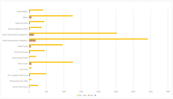
Figure 1.
HyRANK Loukia dataset details.
The WHU-Hi-HongHu dataset was gathered between 16:23 and 17:37 on 20 November 2017, in Honghu City, Hubei Province, China. The data acquisition was conducted using the The DJI Matrice 600 Pro belongs to DJI Innovation Technology Co., Ltd. and is located in Shenzhen, China. equipped with a Nano Hyperspec imaging sensor belongs to Headwall Photonics and is located in Bolton, USA. with a focal length of 17 mm. The weather during the collection was cloudy, with a temperature of approximately 8 °C and a relative humidity of about 55%. A forest-interlaced agricultural system was investigated, featuring hierarchical crop taxonomies ranging from conspecific cultivars (e.g., Chinese cabbage vs. heading cabbage) to phylogenetically divergent Brassica subspecies with distinct phenological traits. Notably, the forest characteristics were prominent, and the same crop types exhibited diversity among different varieties, such as the planting distribution of Chinese cabbage/cabbage and Brassica/small Brassica. The drone was operated at an altitude of 100 m, and the image size was set to 940 × 475 pixels, encompassing 270 bands in the range of 400 to 1000 nm. The spatial resolution of the airborne hyperspectral imagery was approximately 0.043 m. The results are shown in Figure 2.
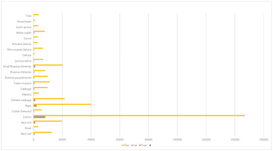
Figure 2.
WHU-Hi-HongHu dataset details.
Acquired through an airborne platform over a 49-min sunset interval, this dataset characterizes spectral patterns across Hanchuan’s transitional ecotone—a rapidly evolving fringe zone demarcating urban expansion boundaries and rural land-use mosaics in the Yangtze River Basin. The dataset was acquired using a Leica Aibot X6 drone equipped with a Nano-Hyperspec imaging sensor with a focal length of 17 mm. The drone was flown at an altitude of 250 m, resulting in an image resolution of 1217 × 303 pixels, covering 274 spectral bands in the range of 400 to 1000 nanometers. Buildings, water bodies, and farmland were included in the study area. Notably, forest-covered regions were prominent, providing rich ground object information for hyperspectral image analysis. The weather during data collection was clear, with a temperature of approximately 30 °C and a relative humidity of about 70%. Due to the low solar elevation angle during the late afternoon collection period, the images contained significant shadowed areas, which may pose challenges for subsequent data analysis. The spatial resolution of the dataset was approximately 0.109 m, offering robust support for hyperspectral image research in fields such as forest monitoring and crop classification. The results are shown in Figure 3.
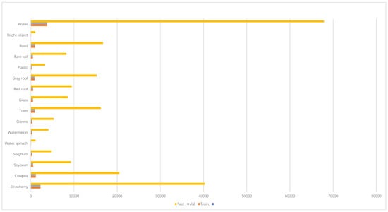
Figure 3.
WHU-Hi-HanChuan dataset details.
The WHU-Hi-LongKou dataset was collected in the afternoon of 17 July 2018, in Longkou Town, Hubei Province, China. The dataset was acquired using a Nano-Hyperspec hyperspectral sensor (8 mm focal length) mounted on a DJI M600 Pro drone platform. The data collection period was from 13:49 to 14:37, under clear and cloudless weather conditions, with a temperature high of 36 °C and a relative humidity of 65%. The study area was predominantly an agricultural landscape, including crops such as corn, cotton, sesame, and different leaf-type soybeans and rice. Additionally, forest patches were interspersed with farmland, providing diverse vegetation cover types, which offered typical samples for analyzing forest canopy spectral characteristics and mixed crop scenarios. The drone was flown at an altitude of 500 m, resulting in an image resolution of 550 × 400 pixels, covering 270 spectral bands in the range of 400–1000 nm with a spatial resolution of approximately 0.463 m. The high spectral resolution and medium-scale spatial resolution of this dataset make it particularly suitable for research in forest vegetation classification, canopy biochemical parameter retrieval, and remote sensing monitoring of agroforestry ecosystems. The results are shown in Figure 4.
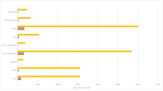
Figure 4.
WHU-Hi-LongKou dataset details.
The WHU-Hi-HongHu dataset, collected in Honghu City, Hubei Province, China, adds a complex agricultural environment dominated by forest landscapes to our study. This dataset is essential to validate the model’s performance in a different geographical and ecological context compared to HyRANK-Loukia. It includes various crop types and forest characteristics, ensuring the model’s effectiveness across diverse conditions. In total, four datasets are involved in this study: WHU-Hi-HongHu, HyRANK-Loukia, WHU-Hi-HanChuan, and WHU-Hi-LongKou. Each dataset offers unique geographical, ecological, and spectral characteristics. This diversity allows us to comprehensively evaluate the model’s performance and robustness across different environmental conditions and land cover types. The use of multiple datasets strengthens the validity of our results and demonstrates the generalizability of the proposed method.
2.2. Methodology
As shown in Figure 5, the proposed WSSGCN classification model consists of four key modules: the watershed superpixel segmentation module, the lightweight multi-scale convolutional module (LMC Module), the adaptive sparse graph modeling module (ASG Module), and the classifier. The overall workflow first generates superpixel regions using the watershed algorithm and constructs a sparse graph structure. Subsequently, lightweight convolution is employed to extract local detail features, while sparse graph modeling is used to capture global semantic relationships. Finally, multi-scale features are fused, and the results are output through the classifier. This framework significantly improves the accuracy and efficiency of hyperspectral image classification through the collaborative optimization of local and global features. Each part is introduced in detail below.
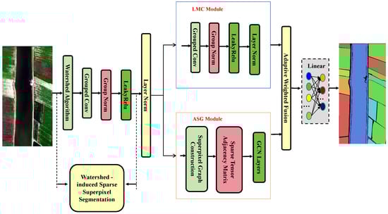
Figure 5.
Workflow of the WSSGCN classification model.
2.2.1. Watershed Superpixel Segmentation Module
The watershed superpixel segmentation module aims to divide hyperspectral images into semantically consistent superpixel regions, providing a foundation for subsequent image structure modeling. PCA is conducted on the hyperspectral dataset to achieve dimensionality reduction and extract dominant spectral features. X retains the first three principal components to reduce redundant information. The reduced dimensional data are obtained as shown in Equation (1):
Remove noise and extract local minima as initial marker points through morphological opening operation. After executing the watershed algorithm, generate a superpixel mask M, as shown in Equation (3):
Each superpixel covers a spatially continuous region of pixels. The superpixel feature matrix F is composed of spectral mean and centroid coordinates as shown in Equation (4):
where is the number of superpixels. Simultaneously, two sparse adjacency matrices are constructed based on adjacency relationships: the Euclidean distance matrix encodes the spectral similarity between superpixels, as shown in Equation (5):
The binary adjacency matrix A describes spatial adjacency and provides a basis for preserving forest boundaries, as shown in Equation (6):
2.2.2. Lightweight Multi-Scale Convolution Module (LMC Module)
The lightweight multi-scale convolution module achieves efficient forest local feature extraction by decoupling spatial and channel dimension feature learning. This module adopts a depthwise separable convolution structure, which first independently performs a 3 × 3 spatial convolution on each channel of the input features to capture local tree crown texture details; subsequently, cross channel information is fused through 1 × 1 convolution to enhance spectral discriminability.
Given the input features as shown in Equation (7):
The output of depthwise separable convolution is as shown in Equation (8):
The output of a 1 × 1 convolution is shown in Equation (9):
The multi-scale activation function combined with LeakyReLU and batch normalization layer adaptively adjusts the weight distribution of different scale features.
2.2.3. Adaptive Sparse Graph Modeling Module (ASG Module)
The adaptive sparse graph modeling module is based on the sparse adjacency matrix generated by the watershed, and dynamically integrates node features and neighborhood information through a gating mechanism. This module first normalizes the superpixel features, and then performs dual path graph convolution, using a Euclidean distance matrix and binary adjacency matrix to model global spectral similarity and spatial adjacency.
Given the superpixel features as shown in Equation (10):
The output of the graph convolution is as shown in Equation (11):
The gating mechanism dynamically suppresses the interference of noisy edges through learnable weights, while preserving the feature contributions of effective neighborhoods. The residual connection and DropPath strategy further enhance the stability of training.
2.2.4. Classifier and Loss Function Design
The classifier outputs the final classification result through multi-level feature fusion and decision output.
Firstly, upsample the superpixel level features output by the ASG module to the original image resolution as shown in Equations (12) and (13):
Channel concatenation is performed with pixel level features extracted by the LMC module to obtain fused features that achieve the fusion of local details and global semantics. The fused features are mapped to the category space through a fully connected layer; Equation (14) for generating category scores is as follows:
The categorical dimensionality K is defined as the cardinality of the target classes, from which probabilistic membership assignments are derived through a Softmax transformation applied to the logit outputs. Equation (15) is as follows:
where represents the probability that the location i,j belongs to category k. A weighted cross-entropy loss function is adopted to balance the problem of class sample imbalance. The class-imbalanced learning scenario necessitates a reformulation of the standard cross-entropy through instance weighting, formally expressed as follows:
This is usually proportional to the reciprocal of the number of class samples. To avoid an overfitting of the model, L2 regularization term constraints are introduced in the loss function. By minimizing the total loss function, the model can simultaneously optimize classification performance and avoid overfitting, thereby improving the accuracy and robustness of hyperspectral image classification.
2.3. Experimental Setup
Our model was developed using Python 3.10 and PyTorch 1.10.1. During the training phase, we utilized an Intel(R) Core(TM) i5-12400F @ 2.50 GHz CPU, an NVIDIA GeForce RTX 3060 GPU, 16 GB DDR4 @ 3200 MHz RAM, and a 512 GB NVMe SSD. To minimize result variability from randomness, each experiment was independently repeated five times with averaged outcomes. For each trial, 20% of samples were randomly selected for training, and the remaining samples were used for testing. Python 3.10 served as the primary programming language, offering extensive library support. PyTorch 1.10.1 was used for building and training neural networks with GPU acceleration. NumPy was utilized for numerical computations, SciPy for scientific computing, OpenCV for image processing, Matplotlib 3.8 for data visualization, and Scikit-learn for data preprocessing and model evaluation. The training process employed a learning rate of 0.001, 100 training epochs, and a batch size of 32. We also implemented a weighted cross-entropy loss function to address class imbalance and incorporated L2 regularization to prevent overfitting.
3. Experimental Results
3.1. Ablation Study
First, ablation experiments were conducted on the WHU-Hi-HongHu dataset to determine the impact of each module in the proposed method. The quantitative results are presented below. The research findings indicate that combining pixel-level CNN with superpixel-level GCN can produce a synergistic effect, enhancing both detailed and holistic feature extraction capabilities. This integration subsequently improves the network’s generalization ability for classification tasks across different datasets. The ablation experiment results are shown in Table 1.

Table 1.
WHU-Hi-HongHu precision table of ablation experiment.
Ablation studies are a crucial part of evaluating the effectiveness of different components in the proposed WSSGCN method. These studies help to understand the individual contribution of each module to the overall performance. A more detailed explanation of the ablation studies follows. The results indicate that the combination of pixel-level CNN and superpixel-level GCN can produce a synergistic effect, enhancing both detailed and holistic feature extraction capabilities. This integration subsequently improves the network’s generalization ability for classification tasks across different datasets. Specifically, the lightweight multi-scale convolution module (LMC Module) plays a significant role in capturing local spatial–spectral features. By using depthwise separable convolution and multi-scale feature extraction, this module enhances the model’s ability to capture complex land cover details. The results show that when only the LMC Module is used, the model achieves an OA of 94.57%. The adaptive sparse graph modeling module (ASG Module) is equally important for modeling global contextual information. Through sparse tensor storage and a gating mechanism, this module significantly reduces the computational overhead of graph convolution while dynamically adjusting the adjacency matrix to suppress noise interference. When only the ASG Module is used, the model achieves an OA of 91.14%, demonstrating its effectiveness in capturing global features. However, when both modules are combined, the model’s performance improves significantly, achieving an OA of 99.66%. This demonstrates the importance of the dual-branch architecture in synergistically optimizing local and global features. The adaptive fusion module is particularly crucial for improving classification accuracy, as it effectively balances the contributions of local and global features through a dynamic weighting strategy. In summary, the ablation studies clearly show that each component of the WSSGCN method contributes to the overall performance improvement. The combination of these components results in a more robust and accurate model for hyperspectral image classification.
3.2. Multi-Method Comparison
From the accuracy table, it can be observed that in GCN, the species of Celtuce and Broad bean remain indistinguishable. This misclassification may be attributed to the limitations of GCN in terms of layer depth, which restricts its ability to explore more distant nodes for comprehensive feature extraction. Additionally, integrating the gating mechanism into GCN enhances classification and generalization capabilities by increasing the network’s attention to remote nodes, enabling it to better capture long-range information in the graph. To evaluate the effectiveness of the proposed method, a comparative analysis was conducted with state-of-the-art deep learning methods for hyperspectral classification. This study employs a variety of comparative approaches for land cover classification, including M3D-DCNN (multi-scale 3D deep convolutional neural network), 3D-CNN (CNN-based 3D deep learning method), DFFN (deep feature fusion network), RSSAN, AB-LSTM (attention-based bidirectional long short-term memory network), SpectralFormer (a transformer-based backbone network), and SSFTT. The experimental results, which are presented in Table 2, Table 3, Table 4 and Table 5, aim to validate the effectiveness and superiority of the proposed model through a comprehensive performance evaluation and analysis.
Table 2.
HyRANK-Loukia classification results table.
Table 3.
WHU-Hi-HongHu classification results table.
Table 4.
WHU-Hi-HanChuan classification results table.
Table 5.
WHU-Hi-LongKou classification results table.
The experimental results demonstrate that the proposed model significantly outperforms other state-of-the-art (SOTA) deep learning-based hyperspectral image (HSI) classification methods across four benchmark HSI datasets. This indicates that the improved algorithm possesses greater potential in handling challenging classification datasets. In terms of inference time, the algorithm represents a highly competitive framework compared to other deep learning approaches. The classification results are shown in Figure 6, Figure 7, Figure 8 and Figure 9.
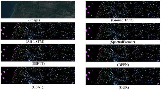
Figure 6.
HyRANK-Loukia dataset classification chart.
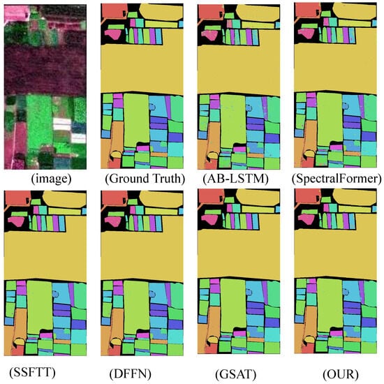
Figure 7.
WHU-Hi-HongHu dataset classification chart.
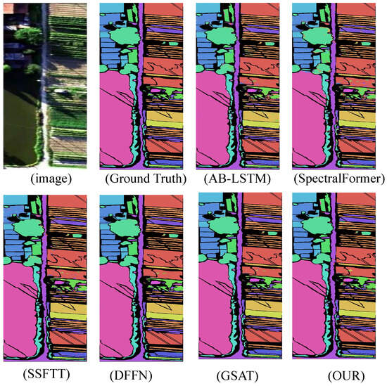
Figure 8.
WHU-Hi-HanChuan dataset classification chart.
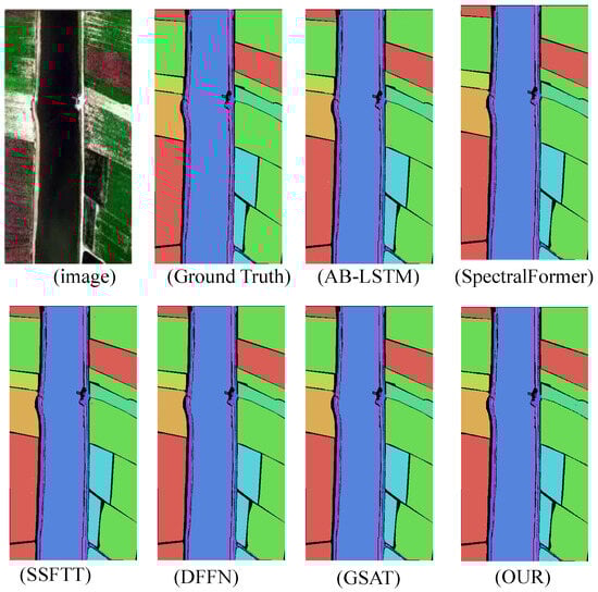
Figure 9.
WHU-Hi-LongKou dataset classification chart.
t-SNE is a dimensionality reduction technique used to map high-dimensional data into a two-dimensional space, enabling the visualization of data distribution and class separation. The figures below Figure 10 illustrate the feature distribution in hyperspectral image classification tasks for four datasets: hrl, WHU-Hi-HanChuan, WHU-Hi-HongHu, and WHU-Hi-LongKou.
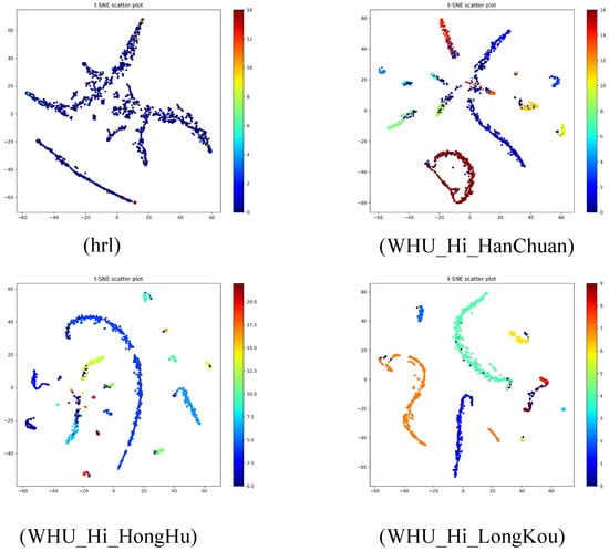
Figure 10.
T-SNE classification maps using algorithms for each dataset.
In the hrl dataset, data points are primarily distributed in two regions: a larger cluster of blue points and a smaller cluster of red points. The blue cluster exhibits high density, while the red cluster shows low density, with a clear separation between them. This indicates that the model has strong discriminative capability in feature extraction for this dataset. In the WHU-Hi-HanChuan dataset, the feature distribution is more scattered, with a high-density red cluster at the center surrounded by multiple low-density blue and green clusters. There is significant overlap between classes, and the boundaries are not well-defined, suggesting that the model has weaker feature discriminability on this dataset, possibly due to class imbalance or data complexity. The WHU-Hi-HongHu dataset exhibits a feature distribution with multiple elongated clusters, primarily consisting of a large blue cluster and several smaller green and red clusters. The blue cluster is well-separated from the others, but there is overlap among the smaller clusters, indicating that the model performs well in extracting features for the main classes but has limited discriminability for minor classes. The WHU-Hi-LongKou dataset also shows a complex feature distribution, with a large blue cluster and multiple smaller green, orange, and red clusters. The blue cluster is somewhat separated from the others, but there is considerable overlap among the smaller clusters, with unclear class boundaries and weak feature discriminability. Overall, the model performs poorly on the WHU-Hi-HanChuan and WHU-Hi-LongKou datasets, with significant feature aliasing, likely influenced by class imbalance or data complexity. Its performance on the WHU-Hi-HongHu dataset is moderate, with good separation for the main classes but limited discriminability for minor classes. The model achieves the best performance on the hrl dataset, demonstrating the most effective class separation.
4. Discussion
The proposed WSSGCN method, which integrates watershed superpixel segmentation with a sparse graph convolutional network, offers an efficient and robust approach to forest hyperspectral image classification. The experimental results from across multiple datasets validate the method’s effectiveness. Technically, the superpixel segmentation module reduces computational complexity through the watershed algorithm while preserving the critical spatial boundary information of forest types, such as coniferous and broadleaf forests. This forms a solid foundation for subsequent graph structure modeling. The dual-branch architecture synergistically optimizes local spatial–spectral features and global contextual information. The lightweight multi-scale convolution module, leveraging depthwise separable convolution and multi-scale feature extraction, enhances the model’s ability to capture intricate land cover details. Simultaneously, the adaptive sparse graph modeling module alleviates the computational burden of graph convolution via sparse tensor storage and a gating mechanism. This module dynamically adjusts the adjacency matrix to mitigate noise interference, further refining the model’s performance.
The quantitative results demonstrate the superiority of the WSSGCN method across multiple evaluation metrics. On the WHU-Hi-HongHu dataset, WSSGCN achieves an overall accuracy (OA) of 99.66%, which is a significant improvement of 3.5% over the SPEFORMER method, along with a Kappa coefficient increase of 0.04. These gains highlight the enhanced classification performance of WSSGCN. Furthermore, the computational efficiency of WSSGCN is markedly better than that of other state-of-the-art methods. For instance, on the same WHU-Hi-HongHu dataset, WSSGCN reduces the training time by approximately 40% and inference time by 30% compared to traditional GCN-based approaches. This is mainly attributed to the sparse tensor-based storage method for the adjacency matrix, which reduces the complexity from quadratic to linear, and the adaptive fusion strategy that dynamically balances local and global features. These improvements not only enhance the accuracy of the model but also make it more practical for real-time applications in resource-constrained scenarios.
t-SNE visualization results provide insights into the model’s feature distribution across different datasets. For instance, the hrl dataset demonstrates exceptional class separation, highlighting the model’s strong discriminative power in simpler scenarios. Conversely, the WHU-Hi-HanChuan and WHU-Hi-LongKou datasets exhibit more pronounced feature aliasing, likely attributable to their complexity, such as containing mixed pixels in urban–rural fringe areas and shadow-covered regions, as well as class imbalance issues. On the WHU-Hi-HongHu dataset, the model shows good separation for major classes but has room for improvement in distinguishing minor classes. Ablation experiments underscore the critical role of the adaptive fusion module in enhancing classification accuracy by dynamically balancing local and global feature contributions.
The complexity of these datasets, including mixed pixels in urban–rural fringe areas and shadow-covered regions, increases spectral variability, making it harder for the model to distinguish between similar classes. For instance, in WHU-Hi-HanChuan, the model exhibits feature aliasing due to the high number of mixed pixels and class imbalance. To address these limitations, future research could optimize the model by introducing an adaptive spectral correction mechanism to handle spectral variability and exploring multimodal data fusion to improve classification capabilities for under-canopy vegetation.
Compared to state-of-the-art deep learning methods like SpectralFormer and SSFTT, WSSGCN exhibits notable advantages in computational efficiency, particularly in resource-constrained settings. Its sparse graph modeling strategy allows it to maintain high accuracy while substantially reducing training and inference time. However, the model still faces challenges in handling scenes with high spectral variability, such as shadow regions in WHU-Hi-HanChuan. Future research directions could include incorporating dynamic spectral correction mechanisms or manifold learning-based nonlinear dimensionality reduction techniques to further enhance the model’s robustness. Additionally, exploring advanced superpixel segmentation algorithms and multimodal data fusion strategies could further improve the model’s classification capabilities for complex forest ecosystems.
5. Conclusions
The WSSGCN method, which combines superpixel segmentation, sparse graph modeling, and dual-branch feature fusion, offers an innovative framework for forest hyperspectral image classification that balances accuracy and efficiency. The experimental results demonstrate that this method outperforms existing mainstream approaches in terms of OA, AA, and the Kappa coefficient on datasets such as WHU-Hi-HongHu and HyRANK-Loukia. On the WHU-Hi-HongHu dataset, the model achieves an OA of 99.66%, thanks to the dataset’s relatively simple structure and distinct spectral characteristics of different land cover types. The model’s dual-branch architecture efficiently captures both local and global features, making it particularly effective for these types of data. Similarly, on the HyRANK-Loukia dataset, the model attains an OA of 85.70%, showing strong performance in classifying complex forest environments. However, the model faces challenges on more complex datasets like WHU-Hi-HanChuan and WHU-Hi-LongKou. On WHU-Hi-HanChuan, the OA drops to 99.00%, while on WHU-Hi-LongKou, it reaches 99.87%. Overall, WSSGCN provides an efficient and scalable solution for hyperspectral remote sensing image classification, with potential applications in precision agriculture, environmental monitoring, and other fields.
For future work, clear directions can be outlined to address these limitations:
- Develop and integrate an adaptive spectral correction mechanism that can dynamically adjust to varying spectral conditions, particularly in shadow regions and areas with high spectral variability;
- Advance the superpixel segmentation algorithm by incorporating deep learning techniques to improve the precision of forest boundary preservation and reduce the loss of important spatial information;
- Explore and implement multimodal data fusion strategies, combining hyperspectral data with LiDAR data to leverage forest height and structural information, thereby enhancing the classification of under-canopy vegetation and improving overall model performance in complex forest environments.
By focusing on these specific areas of improvement, the WSSGCN method can be further refined to handle a broader range of classification challenges, making it a more versatile and powerful tool for hyperspectral remote sensing image classification.
Author Contributions
Investigation, P.C., X.L., X.F., Q.L. and Y.P.; Conceptualization, P.C., X.F. and Y.P.; resources, Y.P., X.F. and Q.L.; methodology, P.C., X.L., X.F., Q.L. and Y.P.; software, P.C., X.L., Q.L. and Y.P.; validation, P.C., X.L., Q.L. and Y.P.; formal analysis, P.C., X.L., X.F. and Y.P.; data curation, P.C., X.L., X.F., Q.L. and Y.P.; writing—original draft preparation, P.C., X.L., X.F., Q.L. and Y.P. All authors have read and agreed to the published version of the manuscript.
Funding
This work is the result of the research project funded by the Guangxi Key Research and Development Program AB24010312. Funded by: Li Qi.
Data Availability Statement
Data are contained within the article.
Conflicts of Interest
The authors declare no conflict of interest.
Abbreviations
The following abbreviations are used in this manuscript:
| GCN | Graph Convolutional Networks |
| SVMs | Support vector machines |
| RNNs | Recurrent neural networks |
| ROI | Region of interest |
References
- Goetz, A.F.; Vane, G.; Solomon, J.E.; Rock, B.N. Imaging spectrometry for earth remote sensing. Science 1985, 228, 1147–1153. [Google Scholar] [CrossRef] [PubMed]
- Mahlein, A.K.; Oerke, E.C.; Steiner, U.; Dehne, H.W. Recent advances in sensing plant diseases for precision crop protection. Eur. J. Plant Pathol. 2012, 133, 197–209. [Google Scholar] [CrossRef]
- Brando, V.E.; Dekker, A.G. Satellite hyperspectral remote sensing for estimating estuarine and coastal water quality. IEEE Trans. Geosci. Remote Sens. 2003, 41, 1378–1387. [Google Scholar] [CrossRef]
- Weng, Q.; Lu, D.; Schubring, J. Estimation of land surface temperature–vegetation abundance relationship for urban heat island studies. Remote Sens. Environ. 2004, 89, 467–483. [Google Scholar] [CrossRef]
- Schaepman, M.E.; Ustin, S.L.; Plaza, A.J.; Painter, T.H.; Verrelst, J.; Liang, S. Earth system science related imaging spectroscopy—An assessment. Remote Sens. Environ. 2009, 113, S123–S137. [Google Scholar] [CrossRef]
- Thenkabail, P.S.; Smith, R.B.; De Pauw, E. Hyperspectral vegetation indices and their relationships with agricultural crop characteristics. Remote Sens. Environ. 2000, 71, 158–182. [Google Scholar] [CrossRef]
- Gao, B.C.; Goetz, A.F. Column atmospheric water vapor and vegetation liquid water retrievals from airborne imaging spectrometer data. J. Geophys. Res. Atmos. 1990, 95, 3549–3564. [Google Scholar] [CrossRef]
- Melgani, F.; Bruzzone, L. Classification of hyperspectral remote sensing images with support vector machines. IEEE Trans. Geosci. Remote Sens. 2004, 42, 1778–1790. [Google Scholar] [CrossRef]
- Ham, J.; Chen, Y.; Crawford, M.M.; Ghosh, J. Investigation of the random forest framework for classification of hyperspectral data. IEEE Trans. Geosci. Remote Sens. 2005, 43, 492–501. [Google Scholar] [CrossRef]
- Camps-Valls, G.; Bruzzone, L. Kernel-based methods for hyperspectral image classification. IEEE Trans. Geosci. Remote Sens. 2005, 43, 1351–1362. [Google Scholar] [CrossRef]
- Toporkov, J.V.; Sletten, M.A. Numerical simulations and analysis of wide-band range-resolved HF backscatter from evolving ocean-like surfaces. IEEE Trans. Geosci. Remote Sens. 2012, 50, 2986–3003. [Google Scholar] [CrossRef]
- Bandos, T.V.; Bruzzone, L.; Camps-Valls, G. Classification of hyperspectral images with regularized linear discriminant analysis. IEEE Trans. Geosci. Remote Sens. 2009, 47, 862–873. [Google Scholar] [CrossRef]
- Fauvel, M.; Tarabalka, Y.; Benediktsson, J.A.; Chanussot, J.; Tilton, J.C. Advances in spectral-spatial classification of hyperspectral images. Proc. IEEE 2012, 101, 652–675. [Google Scholar] [CrossRef]
- Badenas, J.; Sanchiz, J.M.; Pla, F. Motion-based segmentation and region tracking in image sequences. Pattern Recognit. 2001, 34, 661–670. [Google Scholar] [CrossRef]
- Chen, Y.; Jiang, H.; Li, C.; Jia, X.; Ghamisi, P. Deep feature extraction and classification of hyperspectral images based on convolutional neural networks. IEEE Trans. Geosci. Remote Sens. 2016, 54, 6232–6251. [Google Scholar] [CrossRef]
- Hu, W.; Huang, Y.; Wei, L.; Zhang, F.; Li, H. Deep convolutional neural networks for hyperspectral image classification. J. Sens. 2015, 2015, 258619. [Google Scholar] [CrossRef]
- Zhong, Z.; Li, J.; Luo, Z.; Chapman, M. Spectral–spatial residual network for hyperspectral image classification: A 3-D deep learning framework. IEEE Trans. Geosci. Remote Sens. 2017, 56, 847–858. [Google Scholar] [CrossRef]
- Li, W.; Wu, G.; Zhang, F.; Du, Q. Hyperspectral image classification using deep pixel-pair features. IEEE Trans. Geosci. Remote Sens. 2016, 55, 844–853. [Google Scholar] [CrossRef]
- Pržulj, N. Biological network comparison using graphlet degree distribution. Bioinformatics 2007, 23, e177–e183. [Google Scholar] [CrossRef]
- Wang, Y.; Wang, J.; Chen, X.; Chu, T.; Liu, M.; Yang, T. Feature surface extraction and reconstruction from industrial components using multistep segmentation and optimization. Remote Sens. 2018, 10, 1073. [Google Scholar] [CrossRef]
- Zhao, L.; Song, Y.; Zhang, C. T-GCN: A temporal graph convolutional network for traffic prediction. IEEE Trans. Intell. Transp. Syst. 2019, 21, 3848–3858. [Google Scholar] [CrossRef]
- Kipf, T.N.; Welling, M. Semi-supervised classification with graph convolutional networks. arXiv 2016, arXiv:1609.02907. [Google Scholar]
- Chen, Z.; Li, J.; Liu, H.; Wang, X.; Wang, H.; Zheng, Q. Learning multi-scale features for speech emotion recognition with connection attention mechanism. Expert Syst. Appl. 2023, 214, 118943. [Google Scholar] [CrossRef]
- Shuman, D.I.; Narang, S.K.; Frossard, P.; Ortega, A.; Vandergheynst, P. The emerging field of signal processing on graphs: Extending high-dimensional data analysis to networks and other irregular domains. IEEE Signal Process. Mag. 2013, 30, 83–98. [Google Scholar] [CrossRef]
- Bronstein, M.M.; Bruna, J.; LeCun, Y.; Szlam, A.; Vandergheynst, P. Geometric deep learning: Going beyond euclidean data. IEEE Signal Process. Mag. 2017, 34, 18–42. [Google Scholar] [CrossRef]
- Hong, D.; Gao, L.; Yao, J.; Zhang, B.; Plaza, A.; Chanussot, J. Graph convolutional networks for hyperspectral image classification. IEEE Trans. Geosci. Remote Sens. 2020, 59, 5966–5978. [Google Scholar] [CrossRef]
- Venkateswarlu, R. Eye gaze estimation from a single image of one eye. In Proceedings of the Ninth IEEE International Conference on Computer Vision, Nice, France, 14–17 October 2003; pp. 136–143. [Google Scholar]
- Achanta, R.; Shaji, A.; Smith, K.; Lucchi, A.; Fua, P.; Süsstrunk, S. SLIC superpixels compared to state-of-the-art superpixel methods. IEEE Trans. Pattern Anal. Mach. Intell. 2012, 34, 2274–2282. [Google Scholar] [CrossRef]
- Liu, M.Y.; Tuzel, O.; Ramalingam, S.; Chellappa, R. Entropy rate superpixel segmentation. In Proceedings of the CVPR 2011, Colorado Springs, CO, USA, 20–25 June 2011; pp. 2097–2104. [Google Scholar]
- Mou, L.; Lu, X.; Li, X.; Zhu, X.X. Nonlocal graph convolutional networks for hyperspectral image classification. IEEE Trans. Geosci. Remote Sens. 2020, 58, 8246–8257. [Google Scholar] [CrossRef]
- Subudhi, S.; Patro, R.N.; Biswal, P.K.; Dell’Acqua, F. A survey on superpixel segmentation as a preprocessing step in hyperspectral image analysis. IEEE J. Sel. Top. Appl. Earth Obs. Remote Sens. 2021, 14, 5015–5035. [Google Scholar] [CrossRef]
- Stutz, D.; Hermans, A.; Leibe, B. Superpixels: An evaluation of the state-of-the-art. Comput. Vis. Image Underst. 2018, 166, 1–27. [Google Scholar] [CrossRef]
- Defferrard, M.; Bresson, X.; Vandergheynst, P. Convolutional neural networks on graphs with fast localized spectral filtering. Adv. Neural Inf. Process. Syst. 2016, 29, 3844–3852. [Google Scholar]
- Bianchi, F.M.; Grattarola, D.; Alippi, C. Spectral clustering with graph neural networks for graph pooling. In Proceedings of the International Conference on Machine Learning, PMLR, Online, 13–18 July 2020; pp. 874–883. [Google Scholar]
- Li, X.; Fan, X.; Fan, J.; Li, Q.; Gao, Y.; Zhao, X. DASR-Net: Land Cover Classification Methods for Hybrid Multiattention Multispectral High Spectral Resolution Remote Sensing Imagery. Forests 2024, 15, 1826. [Google Scholar] [CrossRef]
- Li, X.; Fan, X.; Li, Q.; Zhao, X. RS-Net: Hyperspectral Image Land Cover Classification Based on Spectral Imager Combined with Random Forest Algorithm. Electronics 2024, 13, 4046. [Google Scholar] [CrossRef]
- Shi, C.; Liao, D.; Zhang, T.; Wang, L. Hyperspectral image classification based on 3D coordination attention mechanism network. Remote Sens. 2022, 14, 608. [Google Scholar] [CrossRef]
- Yin, J.; Qi, C.; Huang, W.; Chen, Q.; Qu, J. Multibranch 3D-dense attention network for hyperspectral image classification. IEEE Access 2022, 10, 71886–71898. [Google Scholar] [CrossRef]
- Wang, L.; Song, Z.; Zhang, X.; Wang, C.; Zhang, G.; Zhu, L.; Li, J.; Liu, H. SAT-GCN: Self-attention graph convolutional network-based 3D object detection for autonomous driving. Knowl. Based Syst. 2023, 259, 110080. [Google Scholar] [CrossRef]
- Diao, Q.; Dai, Y.; Zhang, C.; Wu, Y.; Feng, X.; Pan, F. Superpixel-based attention graph neural network for semantic segmentation in aerial images. Remote Sens. 2022, 14, 305. [Google Scholar] [CrossRef]
- Shen, Y.; Fu, H.; Du, Z.; Chen, X.; Burnaev, E.; Zorin, D.; Zhou, K.; Zheng, Y. GCN-denoiser: Mesh denoising with graph convolutional networks. ACM Trans. Graph. (TOG) 2022, 41, 1–14. [Google Scholar] [CrossRef]
Disclaimer/Publisher’s Note: The statements, opinions and data contained in all publications are solely those of the individual author(s) and contributor(s) and not of MDPI and/or the editor(s). MDPI and/or the editor(s) disclaim responsibility for any injury to people or property resulting from any ideas, methods, instructions or products referred to in the content. |
© 2025 by the authors. Licensee MDPI, Basel, Switzerland. This article is an open access article distributed under the terms and conditions of the Creative Commons Attribution (CC BY) license (https://creativecommons.org/licenses/by/4.0/).