Forest Carbon Storage Dynamics and Influencing Factors in Southeastern Tibet: GEE and Machine Learning Analysis

Abstract

As an important ecological security barrier on the Tibetan Plateau, southeastern Tibet is crucial to maintaining regional carbon balance under climate change. This study innovatively integrates multi-source remote sensing data (Landsat 8, Sentinel-1, and GEDI) on the Google Earth Engine (GEE) platform, and uses machine learning to model forest carbon storage dynamics from 2019 to 2023. The fusion of multi-source data improves forest vertical structure characterization and makes up for the shortage of single optical data. By comparing machine learning algorithms, the Gradient Boosting model performs excellently (validation set R² = 0.909, RMSE = 26.608 Mg/Ha), achieving high-resolution spatiotemporal mapping. The results show significant spatial heterogeneity; the increase in carbon storage in the central and southern regions is mainly in contrast to the scattered decreases in the eastern and western regions, reflecting vegetation restoration and topographic influence. High-altitude areas are subject to climate restrictions and small changes, while low-altitude areas show significant fluctuations due to human activities. Key drivers were elevation (importance score 22.06), slope (17.00), and temperature (22.04). Land use transformation (such as forest expansion) promotes net carbon accumulation and highlights the effectiveness of regional protection policies. This study provides a scientific basis for targeted ecological management of high-altitude ecosystems.

1. Introduction

As the “Third Pole of the World”, the Tibetan Plateau forms a core ecological barrier for China and Asia [1]. The carbon cycle process of its ecosystem plays an irreplaceable regulatory role in the regional and global climate systems. Thanks to the unique geographical and climatic conditions, the forests in southeastern Tibet have developed a mid-low latitude mountain vertical zonal forest ecosystem, forming carbon sink functional areas with significant differences along the altitude gradient. Studies have shown that under the dual influence of global climate change and human activities, the forests in this region exhibit a dual expansion effect: one is the horizontal expansion of the forest into surrounding areas [2], and the other is the upward shift of the forest line in the vertical direction [3,4]. An in-depth analysis of the forest carbon storage in this region is of great scientific value for improving the relevant theories of the carbon cycle and formulating climate-adaptive ecological management strategies.

Among various methods for calculating forest carbon storage, the biomass calculation method that incorporates forest structure parameters has unique advantages [5,6]. The key to accurately assessing carbon stocks lies in constructing a reliable biomass inversion model, and the accuracy of the model directly depends on the level of extraction of forest structural parameters [7]. Due to limited remote sensing data sources, traditional methods for extracting forest structural parameters are often flawed. For example, optical remote sensing is limited by poor penetration capability and weather conditions [8,9], while the application of LiDAR is restricted by the high cost and complexity of forest structure [10,11]. Recent studies have shown that integrating multiple remote sensing data types can significantly improve the accuracy and efficiency of forest parameter extraction [12,13,14]. For example, combining optical and synthetic aperture radar (SAR) data can provide a more comprehensive picture of forest structural characteristics using horizontal texture and vertical height information [15].

With the increasing complexity of multi-source remote sensing data and the ever-increasing requirements of forest structural parameter extraction accuracy, traditional methods gradually expose their limitations in solving multi-scale data coordination and error control. Machine learning techniques can effectively mine spectral, textural, and spatially related features through automatic feature extraction and multidimensional information integration, thus significantly improving the robustness and applicability of forest structural parameter extraction. Recent studies have increasingly adopted machine learning algorithms, such as Random Forests, Support Vector Machines, Gradient Boosting, and decision trees, to improve prediction accuracy and adaptability [16,17]. These algorithms can effectively handle a large number of different remote sensing data, including multispectral satellite images, thermal infrared images, and LiDAR data. By utilizing the rich information in these data, they can learn intricate nonlinear relationships that are difficult to capture by traditional methods. This greatly facilitates the development of forest parameter extraction, such as more accurate estimation of tree height, canopy density, and forest biomass, which ultimately leads to better results for forest parameter extraction [18]. Based on the advancements in forest parameter extraction driven by machine learning technologies, the analytical methods leveraging Google Earth Engine (GEE) harness its powerful cloud-computing capabilities to significantly reduce research costs while enabling the large-scale, high-precision extraction of forest parameters [19,20].

Based on these advances, this study integrates multi-source remote sensing data on the GEE platform, focusing on the forest ecosystem in southeastern Tibet. This method combines optical, SAR, and LiDAR data to address challenges such as cloud interference and terrain complexity. By leveraging machine learning algorithms, we enhance the detection capabilities of forest vertical structures and spatiotemporal carbon dynamics, supporting limited regional carbon monitoring with ground verification. This method improves the accuracy of biomass estimation and demonstrates the potential of ecological management in plateau areas.

Currently, there are numerous research achievements regarding carbon stock estimation, but studies on the spatial variation of carbon stocks and their influencing factors are relatively scarce, especially those related to plateau regions. This study takes forests in southeastern Tibet as the research object and utilizes the Google Earth Engine and machine learning techniques. This study will utilize multi-source remote sensing data using multiple remote sensing classification techniques, including supervised and unsupervised classification, as well as machine learning, in order to classify land cover types and analyze changes over time. This analysis is critical to understanding long-term environmental change and its ecological impacts. Accuracy validation was also carried out to ensure the reliability of remote sensing data interpretation. The results of the classification and change detection were synthesized to generate land cover maps and change reports, which are essential for environmental decision-making and land use planning.

The main objective of this study is to construct a model of spatial and temporal changes in carbon stocks in primary forests of Southeast Tibet, to assess the changes in aboveground carbon stocks, and to analyze the key ecological factors affecting these changes, such as elevation, slope, temperature, wind direction, precipitation, surface air pressure, and land use types over five years. The study will make comprehensive use of satellite remote sensing data and advanced processing techniques to characterize in detail the spatial and temporal characteristics of carbon stock changes from 2019 to 2023, and systematically assess the direct and indirect impacts of climate change and human activities. In addition, the study will explore the importance of establishing national parks and forest reserves for optimizing carbon storage, reducing greenhouse gas emissions, and increasing the carbon sink capacity of ecosystems [21]. In conclusion, this study aims to deepen the understanding of the spatial and temporal dynamics of carbon storage and its drivers in the primary forests of southeastern Tibet and to provide a scientific basis for effective regional carbon management policies.

It should be pointed out that forests in southeastern Tibet are mostly in the mature or overripe stage, with their growth rate tending to slow down and biomass accumulation approaching equilibrium [22,23]. This ecological feature means that the interannual fluctuations in natural carbon storage may be small, and the strict protection policies of local governments (such as limiting logging and ecological restoration projects) further reduce the impact of human interference. However, there are sensor errors, atmospheric correction biases, and uncertainty in multi-source data fusion during remote sensing data inversion, which may affect the accuracy of carbon density estimation. This study systematically discusses such errors in the analysis.

2. Study Area

The southeastern Tibet region (Figure 1) is located in the high mountain and deep valley areas of eastern and southeastern Tibet, as well as northwest Yunnan (Gongshan County). It encompasses administrative territories in both the Tibet Autonomous Region and Yunnan Province, bordered by Sichuan to the east and Qinghai to the north. The geographical coordinates are approximately 27°30′ to 32°32′ N and 91°45′ to 98°56′ E, with an average elevation of about 3000 m and an elevation difference of 7248 m.

The study area is primarily characterized by a humid, subtropical and tropical mountain climate, with an average annual temperature ranging from 12 °C to 18 °C. The number of days with temperatures above 10 °C is approximately 180, with the warmest month averaging 18 °C to 24 °C, and the extreme minimum temperature reaching around −10 °C. The climate is warm with a long frost-free period, abundant heat, and significant rainfall; however, precipitation is unevenly distributed throughout the year, leading to distinct dry and wet seasons. From June to September, over 80% of the annual rainfall occurs.

Over the past 50 years, the southeastern Tibet region has experienced a temperature increase of 0.3 °C to 0.55 °C, alongside a precipitation increase of 20 to 25 mm [24]. Annual precipitation in southeastern Tibet is relatively high, ranging from 400 mm to 800 mm. This high precipitation is primarily attributed to the southwest monsoon, which traverses the Indian Ocean and approaches from the warm and humid regions near the Bay of Bengal, carrying significant heat and moisture toward the Tibetan Plateau. Rainfall in this region predominantly occurs from May to October, with approximately 90% of the May-October rainfall falling between June and September. The influence of the Indian monsoon results in concentrated and abundant precipitation in the southeastern Tibet area [25].

Southeastern Tibet is one of the main distribution areas of forest ecosystems on the Tibetan Plateau. The region is rich in forest vegetation types, including alpine forest line communities, broad-leaved evergreen forest belts, and broad-leaved mixed forest belts. Qinghai fir is the main dominant tree species in the alpine forest line communities in this region [26,27].

The southeastern Tibet presents unique natural environment characteristics due to its unique geography, geomorphology, topography, geology, and hydrometeorological conditions. The climate of the region is strongly influenced by the topography, which gradually becomes drier from the southeast to the northwest, thus forming rich vegetation types and complex ecosystems [28].

3. Material and Methods

The main steps of this study are as follows: First, data acquisition and preprocessing. Multi-source remote sensing data such as Landsat and Sentinel-1 were used, and operations such as cropping and calibration were performed to ensure data quality. Then, key surface features such as vegetation index were extracted from the preprocessed data. Subsequently, machine learning techniques—including regression-oriented approaches such as Random Forest and Gradient Boosting—were used to analyze the images, model continuous carbon stock variables, and detect spatiotemporal changes in land cover. Next, the accuracy of the remote sensing image analysis results is verified. Then, the results are integrated to generate land cover maps and change reports. Finally, post-processing is performed to generate statistical reports and visualize data to facilitate the understanding and application of the research results. The processing flowchart is shown in Figure 2.

3.1. Data Source

3.1.1. Landsat 8 Data

Landsat 8 data products are provided by Landsat 8 satellites jointly managed by the United States Geological Survey (USGS) and NASA. The data of Collection 2 Level 2 include both the surface reflectivity of the multispectral band and the surface temperature of the thermal infrared band. The data include atmospheric and geometric corrections to provide more accurate surface reflectivity information [29]. Additionally, Tier 1 data typically include preprocessed radiance and reflectance data. Therefore, this study selects the Landsat 8 Tier 1 reflectance dataset using the C02 version, which has undergone atmospheric and geometric corrections to provide more precise surface reflectance information. Such datasets are commonly used in remote sensing applications for surface monitoring, environmental research, and resource management.

The research employs Landsat 8 satellite data for the southeastern region of Tibet from 2019 to 2023, with a spatial resolution of 30 m. The data are sourced from the USGS Earth Explorer (https://earthexplorer.usgs.gov/, accessed on 20 July 2023) as Tier 1 terrain-corrected products, which have been subjected to radiometric and geometric corrections, with selected images being cloud-free or with less than 2% cloud cover. Each data period contains seven bands (Band 1 to Band 7), organized sequentially by spring, summer, and autumn data to form a dataset comprising 21 bands in total.

3.1.2. Sentinel-1 Data

The Sentinel-1 data products are from the Copernicus Sentinel-1 satellite, part of the European Space Agency (ESA). The experiment in this study utilized Sentinel-1’s imaging mode and band as the Interferometric Wide Swath mode, with a pixel size of 10 m × 10 m. The selected data type is GRD (Ground Range Detected), a radar data product type from Sentinel-1 satellite that undergoes geometric correction to convert radar signals from slant range to ground range coordinates, enabling accurate georeferencing and quantitative analysis of surface features. The Sentinel-1 data have a high resolution of 40 m × 40 m and an all-weather observing capability, which makes it particularly suitable for monitoring cloud-covered areas.

The Sentinel-1 satellite carries a synthetic aperture radar (SAR) sensor, which can penetrate the clouds to obtain surface information and is particularly suitable for monitoring parameters such as forest cover change, canopy height, and forest depression [30]. The fusion of SAR data with optical remote sensing data can improve the accuracy and reliability of the extraction of forest structural parameters [31].

3.1.3. ERA5 Meteorological Data

The ECMWF (European Centre for Medium-Range Weather Forecasts) is an international meteorological research organization. ERA5 is an atmospheric reanalysis dataset produced and maintained by ECMWF, which provides global coverage of meteorological and climatic data. This study utilized ERA5 terrestrial reanalysis data, which provide detailed global meteorological and climatic information, including temperature, precipitation, and wind speed. These data are valuable for analyzing forest growth environments, modeling dynamic processes, and assessing spatial distribution and seasonal variations in forest structural parameters.

3.1.4. GEDI Data

We selected the GEDI04_B_002 dataset, a Level 4B gridded aboveground biomass density product provided by NASA’s Global Ecosystem Dynamics Investigation (GEDI) mission. This dataset is derived from GEDI’s L2A and L2B observations, statistically aggregated into a 1 km × 1 km global grid, and is primarily used to study forest carbon storage, vegetation height, and ecosystem structure. GEDI is an advanced airborne LiDAR system specialized in the extraction of forest structural parameters, such as tree height, canopy cover, biomass, etc., on a global scale [32]. The use of GEDI data in combination with optical remote sensing data can significantly improve the accuracy and efficiency of forest structural parameter extraction [33].

3.1.5. SRTM Data

We used the Shuttle Radar Topography Mission (SRTM) version 3 (SRTM v3) digital elevation model (DEM) at 30 m spatial resolution (SRTM1 product) over southeastern Tibet. The dataset was obtained from NASA’s Earthdata portal (https://earthdata.nasa.gov/, accessed on 20 July 2023) and provides elevation data in meters with a vertical accuracy of <16 m. The data were collected in February 2000 using interferometric synthetic aperture radar (InSAR) aboard the Space Shuttle Endeavour, covering 60° N–56° S at 1-arcsecond (~30 m) resolution. This high-resolution DEM was essential for analyzing terrain effects on forest structure in our study area.

3.1.6. ESA Data

We used the ESA WorldCover 10 m 2020 product (v100), which provides global land cover classification at a 10 m spatial resolution (ESA, 2021). The dataset, derived from Sentinel-1 (SAR) and Sentinel-2 (optical) data, categorizes land cover into 11 classes, including forest, cropland, and urban areas. The data cover our study area in southeastern Tibet and were accessed through the ESA WorldCover project under the Earth Observation Envelope Programme (EOEP-5).

Although multi-source remote sensing data (Landsat 8, Sentinel-1, GEDI) provide large-scale continuous observation capabilities, their inherent errors may affect the inversion results. For example, Landsat 8 surface reflectance data are affected by atmospheric correction residual errors, Sentinel-1SAR data are prone to geometric distortions in complex terrain areas, and GEDI LiDAR’s 1 km resolution may smooth out local heterogeneity. In addition, the loss of temporal data caused by cloud coverage should be carefully considered in the interpretation of the results.

A summary of the aforementioned datasets is provided in

Table 1. An introduction to the dataset.

Data and Version	Data Content	Resolution
Landsat 8 Collection 2 Level 2 Tier 1	Reflectance data, atmospheric and geometric correction	30 m
Sentinel-1	Synthetic aperture radar (SAR) data	10 m
ERA5 Daily Data	Temperature, precipitation, pressure, wind speed, etc.	9000 m
GEDI Level 4B	LiDAR system, biomass	1000 m
SRTM GL1 v003	Elevation data	30 m
ESA v100	Global land cover map	10 m

. In this study, a spatial resolution of 1000 m × 1000 m was selected. However, for the analysis of the influence of land use types and climatic factors (ERA5 Daily Data) on biomass in southeastern Tibet (Section 4.5 and Section 4.6), a coarser resolution of 9000 m × 9000 m was adopted in the laboratory experiments.

3.2. Research Methods

3.2.1. Machine Learning Algorithms

This study employed a variety of machine learning algorithms to extract forest structural parameters. The algorithms utilized include Random Forest, CART decision tree, Gradient Boosting, and Support Vector Machine (SVM).

Random Forest is an ensemble learning method that performs regression tasks by constructing multiple decision trees [34]. Each decision tree is trained independently, and their results are aggregated to obtain the final prediction. The core ideas of the Random Forest algorithm include two aspects: firstly, using bootstrap sampling to generate subsets of the training dataset; secondly, randomly selecting a subset of variables for splitting at each node instead of choosing the optimal splitting variable. This approach can effectively reduce the risk of overfitting and improve the model’s generalization ability. The main advantages of the Random Forest algorithm are high accuracy, the ability to handle a large number of input variables efficiently, and a relatively low susceptibility to overfitting. It is suitable for regression tasks. In this study, the bootstrap sampling algorithm is selected, and the output mode is set to regression.

CART is a widely used decision tree algorithm. It recursively partitions the dataset to form a series of rules, ultimately achieving regression prediction of the data. The CART decision tree algorithm constructs a complete tree by selecting optimal features and split points at each node to minimize squared error [35], ensuring each split optimizes the fit to continuous target values and balances model complexity with predictive accuracy.

Gradient Boosting is an ensemble learning method that combines weak learners into a strong learner. It iteratively optimizes in the direction of the negative gradient of the loss function, gradually adding new decision trees to the model to reduce the overall prediction error. The key to Gradient Boosting lies in how to efficiently estimate the gradient of the loss function and how to choose appropriate splitting points. Gradient Boosting typically achieves high accuracy but involves complex parameter tuning and may require longer training times.

The SVM algorithm is commonly used for classification and regression analysis. Its basic goal is to find an optimal hyperplane that maximizes the separation between samples of different classes. SVM seeks the optimal hyperplane by maximizing the margin, where the margin refers to the distance from the closest data point to the hyperplane. When dealing with nonlinear regression problems, SVM can transform data into a high-dimensional space by introducing kernel methods, thereby constructing a function that better models the nonlinear relationship between inputs and continuous outputs. The SVM algorithm exhibits strong capabilities for handling nonlinear regression and can address complex data patterns through kernel functions. However, its performance may decline when the number of features far exceeds the number of samples.

The implementation and validation of these algorithms are detailed in Section 3.2.2.

3.2.2. Model Implementation

This study integrates Landsat 8 data, Sentinel-1 data, ERA5 meteorological data, and GEDI data to create a new dataset, with 70% designated as the training set and 30% as the validation set. Random sampling is performed on the training set for input into the model, encompassing two dimensions: rows (individual samples) and columns (feature variables). Row sampling employs the bootstrap sampling algorithm with a sampling rate of 100%, resulting in a sample size of 1000, and biomass is selected as the feature variable. Based on these steps, the final prediction results are obtained by calculating the mean values.

The vertical axis represents the predicted biomass, while the horizontal axis represents the observed biomass. Using the Random Forest algorithm, a corresponding scatter plot is generated. A trend line is added based on the distribution of the scatter points to develop a biomass prediction model for the aboveground biomass in the southeastern region of Tibet. Using the GEE platform, the number of trees, the maximum number of nodes of each tree, and the minimum number of samples of each leaf node were determined through multiple tests. Subsequently, the regression models were implemented in the Random Forest algorithm, CART decision tree algorithm, Gradient Boosting algorithm, and Support Vector Machine algorithm, where the models were used as the core prediction functions within these algorithms to predict the verification samples.

3.2.3. Evaluation Metrics

In this study, the coefficient of determination (R²), root mean square error (RMSE), mean absolute error (MAE), relative prediction deviation (RPD), and mean absolute percentage error (MAPE) were used to evaluate the model fitting.

The coefficient of determination (R²) indicates the proportion of the variance of the dependent variable that is explained by the independent variables [36]. The larger the R², the better the model fit as shown in Equation (1).

The formulas for the above evaluation metrics are as follows:

$$R^2={\displaystyle \frac{{\displaystyle \sum _{\mathrm{i}=1}^n{({\widehat{y}}_{\mathrm{i}}-\overline{y})}^2}}{{\displaystyle \sum _{\mathrm{i}=1}^n{(y_i-\overline{y})}^2}}}$$

(1)

In the formula, ${\widehat{y}}_{\mathrm{i}}$ represents the predicted value; $y_i$ represents the measured value of the sample plot; $\overline{y}$ represents the mean of the measured values of the sample plots; and $n$ represents the number of training and validation sample plots.

The root mean square error (RMSE) is the arithmetic square root of the standard error and measures the deviation between the predicted value and the actual value. The smaller the RMSE, the stronger the prediction ability and the better the model performance, as shown in Equation (2).

$$RMSE=\sqrt{{\displaystyle \frac{1}{n}}{\displaystyle \sum _{i=1}^n{(y_i-{\widehat{y}}_i)}^2}}$$

(2)

In the formula, ${\widehat{y}}_i$ denotes the predicted value; $y_i$ represents the measured value of a specific observation point; and $n$ stands for the total number of observation points.

The mean absolute error (MAE) measures the predictive performance of the model by calculating the mean of the absolute difference between the predicted value and the actual value. The smaller the MAE, the higher the prediction accuracy, as shown in Equation (3).

$$MAE={\displaystyle \frac{1}{n}}{\displaystyle \sum _{i=1}^n\left|y_i-{\widehat{y}}_i\right|}$$

(3)

In the formula, $y_i$ represents the measured value of an observation point (or sample plot); ${\widehat{y}}_i$ denotes the predicted value corresponding to that observation point; and $n$ stands for the total number of observation points.

The relative prediction deviation (RPD) is the ratio of the standard deviation of the measured value to the standard deviation of the difference between the predicted value and the measured value. The higher the RPD value, the better the variability of the model’s prediction performance relative to the observed data. Usually, an RPD value greater than 1.5 means that the model’s prediction performance is good, as shown in Equation (4).

$$RPD={\displaystyle \frac{S{D}_{observed}}{S{D}_{residuals}}}$$

(4)

In the formula, $S{D}_{observed}$ represents the standard deviation of the observed values; and $S{D}_{residuals}$ denotes the standard deviation of the differences between the predicted values and the observed values.

The mean percentage absolute error (MAPE) measures the average ratio of the absolute error to the actual value at each point; the smaller the MAPE, the higher the prediction accuracy of the model and the smaller the prediction error, as shown in Equation (5).

$$MAPE=\left({\displaystyle \frac{1}{n}}{\displaystyle \sum _{i=1}^n\left|\frac{y_i-{\widehat{y}}_i}{y_i}\right|}\right)\times 100\%$$

(5)

In the formula, $y_i$ represents the measured value of a sample plot (or observation point); ${\widehat{y}}_i$ denotes the predicted value corresponding to that sample plot (or observation point); and $n$ stands for the total number of observation points (or sample plots).

3.2.4. Carbon Stock Calculation

The carbon stock is calculated by multiplying the obtained biomass by a conversion factor, which reflects the relationship between biomass and carbon stock [37]. Through calculations, the conversion factor is determined to be 0.5 (dimensionless, assuming a 50% carbon content in biomass), resulting in a thematic map of carbon stock [38]. It is observed that some regions in the thematic map of carbon stock are missing. To address this, the unmasking method is employed to obscure and fill in the carbon stock, with the vacant areas filled with zeros, and finally, this layer is added to the map.

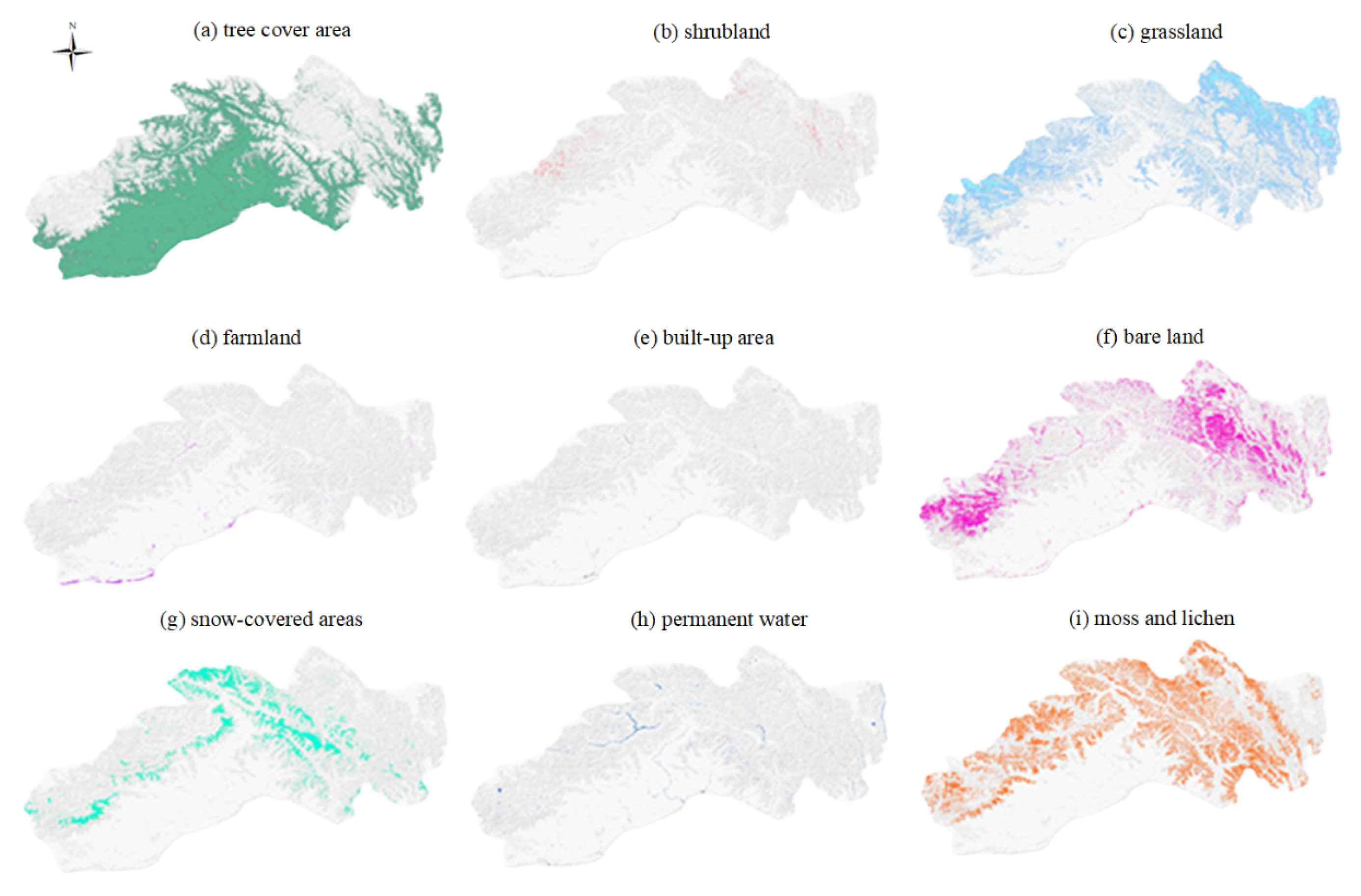
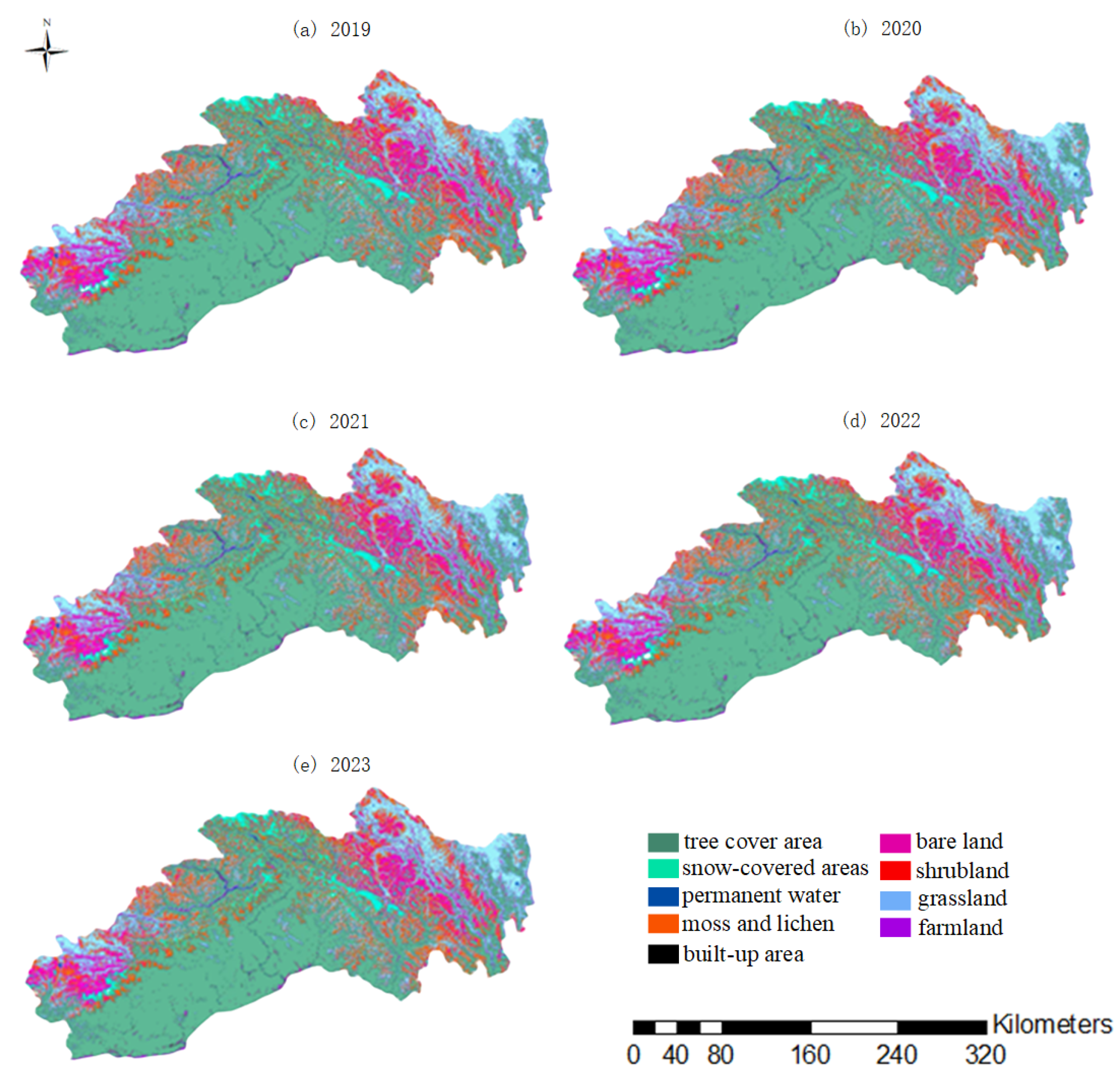
3.2.5. Land Use Types

Land use data are sourced from the ESA, and acquired through classification system adjustments, patch modifications, and dynamic updates, with a spatial resolution of 10 m. Based on this classification system, land use raster maps for the years 2019, 2020, 2021, 2022, and 2023 are extracted through masking, and land use types are reclassified into forest cover, shrub areas, grasslands, agricultural land, built-up areas, bare land/sparse vegetation, snow and ice surfaces, permanent water bodies, and moss and lichen. Temporal changes in land use types are analyzed to identify transitions between classes and their associations with carbon storage dynamics.

4. Results

4.1. Machine Learning Model Results

In the study conducted on the Google Earth Engine platform for extracting forest structural parameters in southeastern Tibet, prediction models for aboveground biomass were developed using the Random Forest algorithm, CART decision tree algorithm, Gradient Boosting algorithm, and Support Vector Machine (SVM) algorithm. Comparative analyses of the results from the training and validation sets of each model were performed to determine the optimal algorithm for subsequent research. The aboveground biomass prediction models for the southeastern region of Tibet, derived from the Random Forest model, CART decision tree algorithm, Gradient Boosting algorithm, and Support Vector Machine algorithm, along with their respective metrics, are summarized in

Table 2. Training and prediction results of machine learning models.

Evaluation Indicators		R2	RMSE (Mg/Ha)	MAE (Mg/Ha)	RPD (Mg/Ha)	MAPE (%)
Random Forest	Training Set	0.940	22.762	18.030	4.009	25.789
	Validation Set	0.901	27.799	21.854	3.166	26.560
CART Decision Tree	Training Set	0.920	25.710	19.328	3.524	24.739
	Validation Set	0.861	32.823	25.508	2.681	29.934
Gradient Boosting	Training Set	0.957	19.336	15.087	4.753	21.612
	Validation Set	0.909	26.608	20.302	3.308	23.626
Support Vector Machine	Training Set	0.560	71.234	58.020	1.280	80.680
	Validation Set	0.365	78.021	64.683	1.155	82.641

.

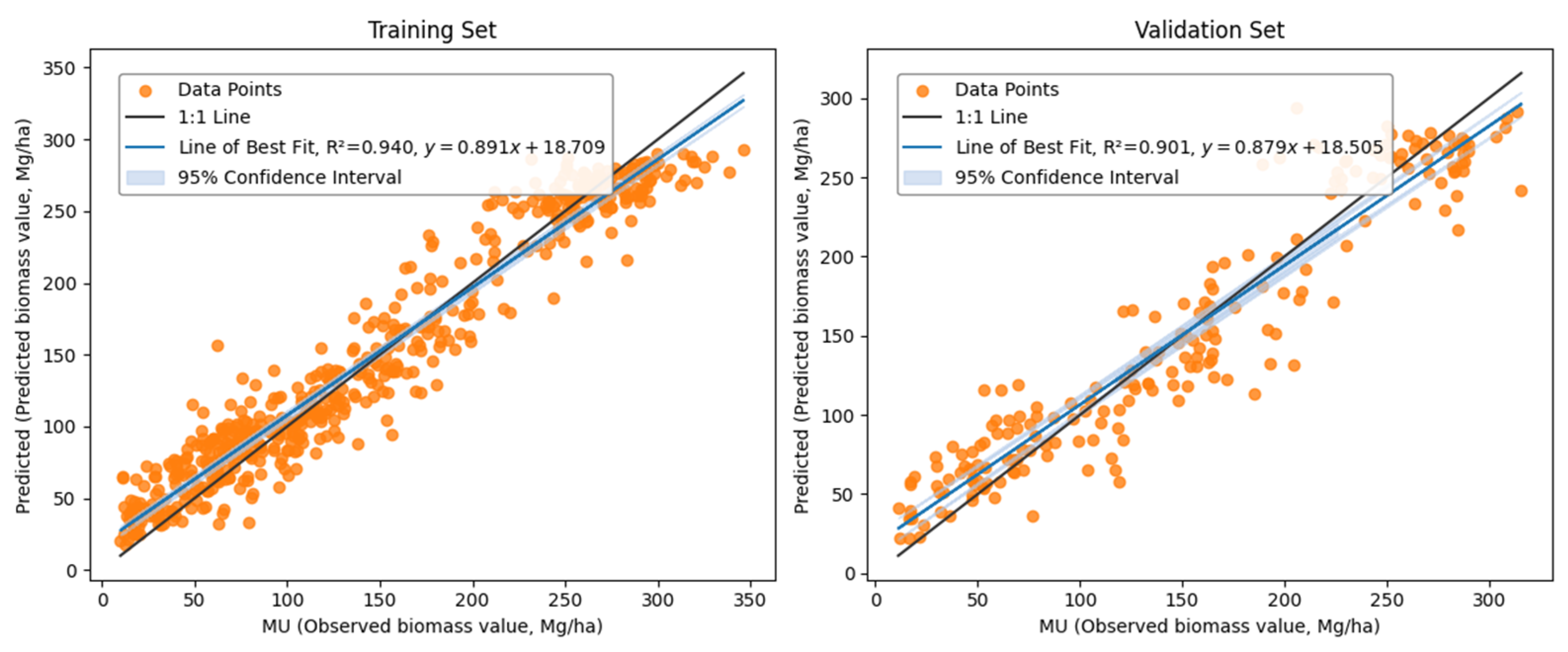
4.1.1. Random Forest Algorithm Model

Through multiple trials, the key parameters of the Random Forest model are adjusted, with the number of decision trees ultimately determined to be 100, the maximum number of nodes per tree to be 15, the minimum sample size for each leaf node to be 8, the feature subsample size to be 3, and the node splitting strategy based on optimal gain. The resulting aboveground biomass prediction model for the southeastern region of Tibet for the training and validation sets is illustrated in Figure 3.

The left figure displays the relationship between the predicted values (Predicted) and the observed values (MU) in the training dataset. The linear regression equation is given by Predicted = 0.891 × MU + 18.709, indicating that the predicted values are 0.89 times the observed values plus a constant of 18.709. The coefficient of determination (R²) is 0.940, the root mean square error (RMSE) is 22.762, the mean absolute error (MAE) is 18.030, the relative prediction deviation (RPD) is 4.009, and the mean absolute percentage error (MAPE) is 25.789. This suggests that the model fits well into the training set and can explain a significant portion of the variability.

The right figure displays the relationship between the predicted values (Predicted) and the observed values (MU) in the validation dataset. The linear regression equation is Predicted = 0.879 × MU + 18.505, indicating that the predicted values are 0.879 times the observed values plus a constant of 18.505. The coefficient of determination (R²) is 0.901, the root mean square error (RMSE) is 22.799, the mean absolute error (MAE) is 21.854, the relative prediction deviation (RPD) is 3.166, and the mean absolute percentage error (MAPE) is 26.560. These metrics suggest that the model performs exceptionally well in extracting forest structural parameters on the training set.

4.1.2. CART Decision Tree Algorithm Model

Through multiple trials, the key parameters of the CART model are adjusted, and we ultimately determined the number of decision trees to be 100, the maximum number of nodes per tree to be 100, the minimum sample size for each leaf node to be 10, and the feature subsample size to be 3, with the node splitting strategy based on optimal gain. The resulting aboveground biomass prediction model for the southeastern region of Tibet for both the training and validation sets is illustrated in Figure 4.

The left figure shows the relationship between the predicted values (Predicted) and the observed values (MU) in the training dataset. The linear regression equation is given by Predicted = 0.926 × MU + 12.345, indicating that the predicted values are 0.926 times the observed values plus a constant of 12.345. The coefficient of determination (R²) is 0.920, the root mean square error (RMSE) is 25.710, the mean absolute error (MAE) is 19.328, the relative prediction deviation (RPD) is 3.524, and the mean absolute percentage error (MAPE) is 24.739. This indicates that the model fits well into the training set and is capable of explaining a substantial portion of the variability.

The right figure displays the relationship between the predicted values (Predicted) and the observed values (MU) in the validation dataset. The linear regression equation is Predicted = 0.866 × MU + 19.639, indicating that the predicted values are 0.866 times the observed values plus a constant of 19.639. The coefficient of determination (R²) is 0.861, the RMSE is 32.823, the MAE is 25.508, the RPD is 2.681, and the MAPE is 29.934. This suggests that the model demonstrates excellent performance in extracting forest structural parameters in the training set.

It is worth noting that the scatter plot presents a vertical grouping phenomenon where multiple observations correspond to the same predicted value, which is an inherent feature of the CART decision tree architecture. This phenomenon originates from the mechanism of the CART setting the predicted value as the average of samples within each leaf node, resulting in a segmented constant characteristic of the output. Although parameters were optimized in the study (such as increasing the maximum number of nodes and reducing the minimum number of leaf node samples to achieve finer-grained splitting), a single tree structure still struggles to resolve samples with similar feature combinations but slight differences in observed values, resulting in these discrete clusters. This phenomenon is a natural result of CART recursive partitioning strategy, not a data or analysis flaw.

4.1.3. Gradient Boosting Algorithm Model

After multiple experiments to adjust the key parameters of the Gradient Boosting model, the final configuration includes 50 decision trees, a maximum node count of 50 per tree, a minimum sample size of 10 per leaf node, a learning rate of 0.1, and a sampling rate of 0.8. The resulting aboveground biomass prediction model for the southeastern region of Tibet for both the training and validation sets is shown in Figure 5.

The left figure illustrates the relationship between the predicted values (Predicted) and the observed values (MU) in the training dataset. The linear regression equation is Predicted = 0.923 × MU + 14.479, indicating that the predicted values are 0.923 times the observed values plus a constant of 14.479. The coefficient of determination (R²) is 0.957, the RMSE is 19.336, the MAE is 15.087, the RPD is 4.753, and the MAPE is 21.612, which indicates strong fitting performance on the training set, capable of explaining most of the variability.

The right figure shows the relationship between the predicted values (Predicted) and the observed values (MU) in the validation dataset. The linear regression equation is Predicted = 0.907 × MU + 14.666, indicating that the predicted values are 0.907 times the observed values plus a constant of 14.666. The coefficient of determination (R²) is 0.909, the RMSE is 26.608, the MAE is 20.302, the RPD is 3.308, and the MAPE is 23.626, confirming that the model performs exceptionally well in extracting forest structural parameters.

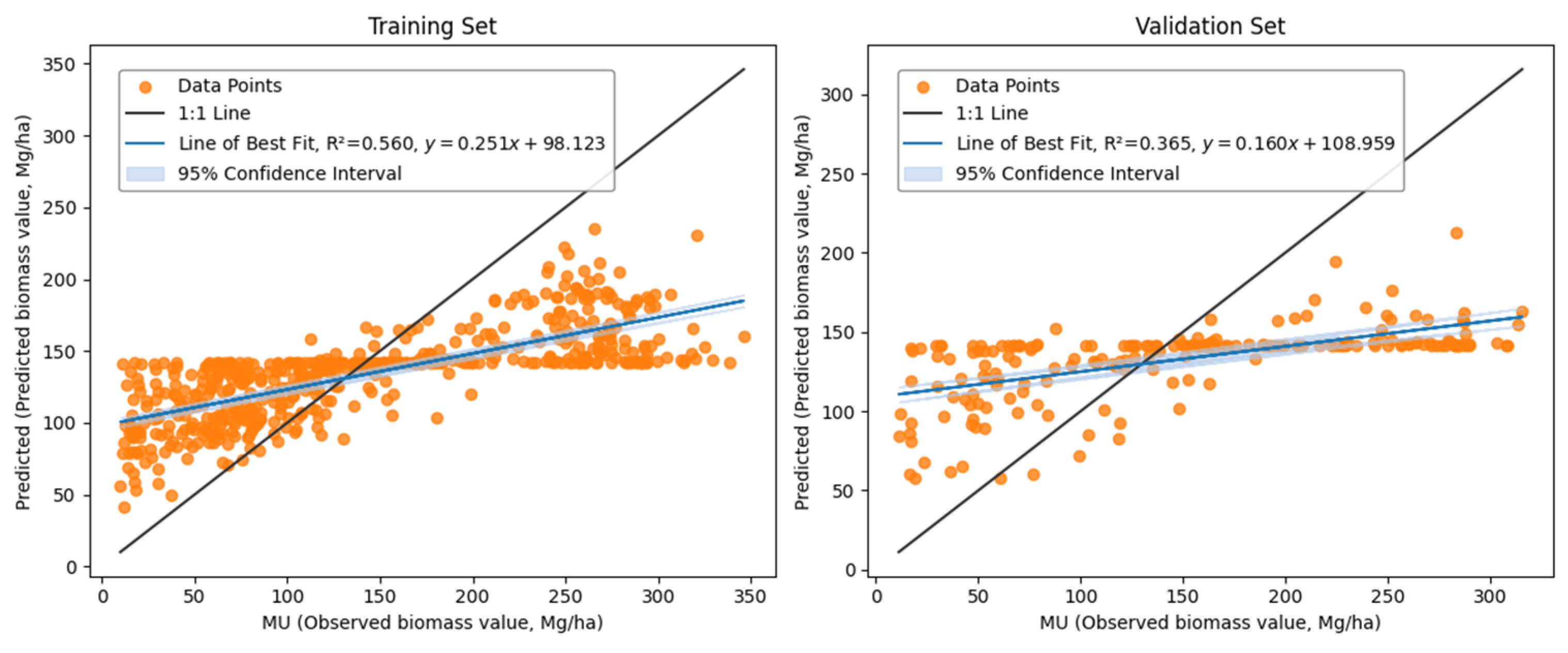
4.1.4. Support Vector Machine Algorithm Model

Through multiple trials, the key parameters of the SVM model were adjusted, ultimately determining the kernel function type to be “RBF”, the SVM type to be “NU_SVR”, the cost parameter to be 50, and the ν parameter to be 0.6. The resulting aboveground biomass prediction model for the southeastern region of Tibet for both the training and validation sets is illustrated in Figure 6.

The left figure shows the relationship between the predicted values (Predicted) and the observed values (MU) in the training dataset. The linear regression equation is Predicted = 0.251 × MU + 98.123, indicating that the predicted values are 0.251 times the observed values plus a constant of 98.123. The coefficient of determination (R²) is 0.560, the RMSE is 71.234, the MAE is 58.020, the RPD is 1.280, and the MAPE is 80.680, suggesting that the model fits well on the training set and explains a significant portion of the variability.

The right figure displays the relationship between the predicted values (Predicted) and the observed values (MU) in the validation dataset. The linear regression equation is Predicted = 0.160 × MU + 108.959, indicating that the predicted values are 0.160 times the observed values plus a constant of 108.959. The coefficient of determination (R²) is 0.365, the RMSE is 78.021, the MAE is 64.683, the RPD is 1.155, and the MAPE is 82.641, indicating that the model performs exceptionally in extracting forest structural parameters in the training set.

Among these models, the Gradient Boosting algorithm achieves the highest R² and RPD values, while exhibiting the lowest RMSE, MAE, and MAPE, indicating superior fitting performance. Conversely, the Random Forest, CART decision tree, and Support Vector Machine algorithms all present lower R² and RPD values, along with higher RMSE, MAE, and MAPE, than the Gradient Boosting algorithm. Therefore, the Gradient Boosting algorithm was selected for subsequent research due to its outstanding fitting performance.

4.2. Forest Biomass Change Results

This study utilizes imagery data from the southeastern region of Tibet and employs the Gradient Boosting algorithm to derive the aboveground biomass distribution for the years 2019, 2020, 2021, 2022, and 2023, as illustrated in Figure 7.

From Figure 7, it is evident that the southwestern part of the southeastern Tibet region exhibits more vigorous growth, while the northeastern and northwestern parts show sparser vegetation. This growth pattern is linked to the topography of the region, where the northeastern and northwestern areas have poor soil and are characterized by numerous mountains, which are unfavorable for growth. In contrast, the southwestern region demonstrates a gradual increase in density, with vegetation becoming denser from the southwest to the northeast and from the southeast to the northwest. Overall, the southeastern region of Tibet shows a trend of higher elevations in the southwest and lower elevations in the northeast. The biomass change from 2019 to 2023 reveals a balanced increase and decrease, indicating that the forest development in this area is relatively mature, with overall vegetation cover tending toward stability and a slowly increasing trend.

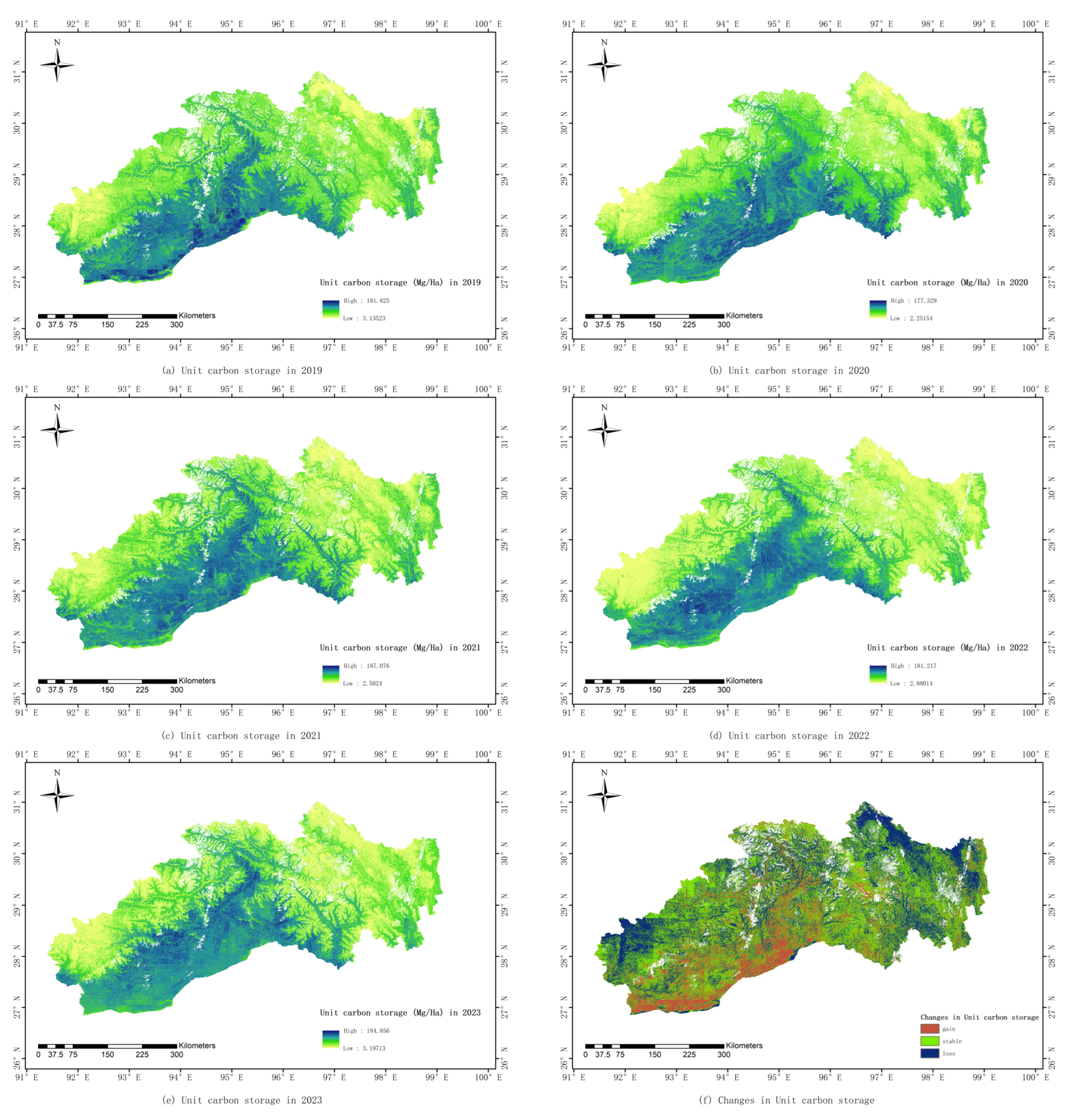
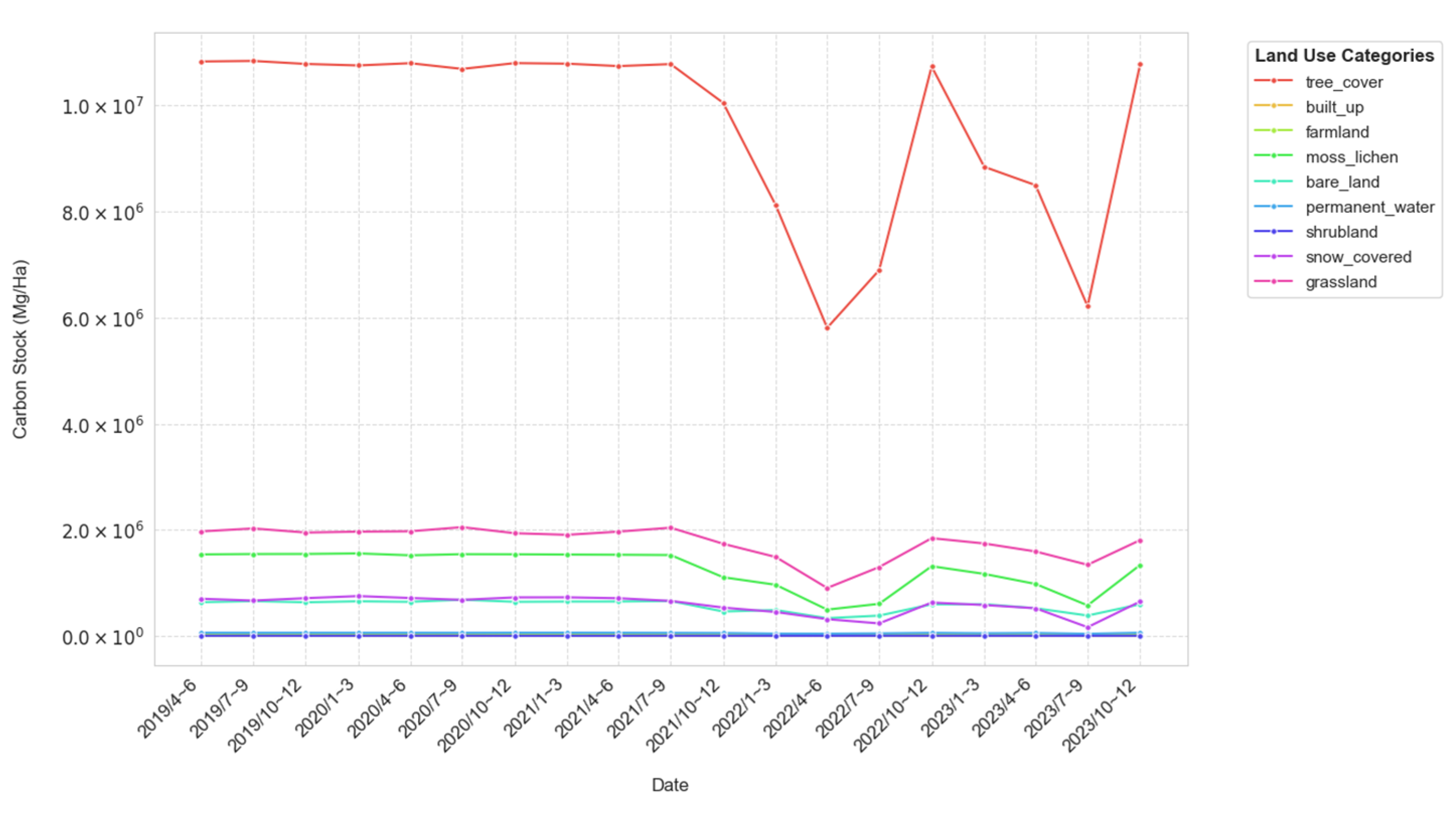
4.3. Temporal Changes in Forest Carbon Stocks

Figure 8 and

Table 3. Carbon density and study area.

Date	Carbon Density (Mg/Ha)	Study Area (m2)
2019/4~6	75.46	1.82 × 1011
2019/7~9	75.75	1.82 × 1011
2019/10~12	75.22	1.82 × 1011
2020/1~3	75.48	1.82 × 1011
2020/4~6	75.33	1.82 × 1011
2020/7~9	75.32	1.82 × 1011
2020/10~12	75.31	1.82 × 1011
2021/1~3	75.13	1.82 × 1011
2021/4~6	75.10	1.82 × 1011
2021/7~9	75.40	1.82 × 1011
2021/10~12	77.06	1.58 × 1011
2022/1~3	73.12	1.38 × 1011
2022/4~6	72.35	9.58 × 1010
2022/7~9	71.05	1.17 × 1011
2022/10~12	75.79	1.75 × 1011
2023/1~3	72.68	1.56 × 1011
2023/4~6	72.50	1.47 × 1011
2023/7~9	71.40	1.07 × 1011
2023/10~12	76.64	1.74 × 1011

present the quarterly carbon density (Mg/Ha) and the area of the study region (m²) from 2019 to 2023.

From the carbon density data, it is evident that between 2019 and 2023, the minimum carbon density was recorded at 71.05 Mg/Ha in the third quarter of 2022, while the maximum reached 77.06 Mg/Ha in the fourth quarter of 2021. The maximum fluctuation during this period was 6.01 Mg/Ha, with an average carbon density of approximately 74.53 Mg/Ha. Overall, the carbon density exhibited a steady upward trend from 2019 to 2021, peaking at 77.06 Mg/Ha in the fourth quarter of 2021. In 2022, the carbon density slightly decreased to a low of 71.05 Mg/Ha (third quarter) before rebounding to 75.79 Mg/Ha (fourth quarter). In 2023, the carbon density fell again to 71.40 Mg/Ha (third quarter) but later rose to the peak of 76.64 Mg/Ha in the fourth quarter.

The area of the study region mirrored the fluctuations in carbon density, with the lowest area of 9.58 × 10¹¹ m² recorded in the second quarter of 2022 and the highest area of 1.82 × 10¹¹ m² in the fourth quarter of 2022, averaging around 1.63 × 10¹¹ m². The significant decline in the area early in 2022 to 9.58 × 10¹⁰ m², followed by a gradual recovery, reflects disturbances likely related to cloud interference during carbon stock calculations, as areas obscured by clouds were not included.

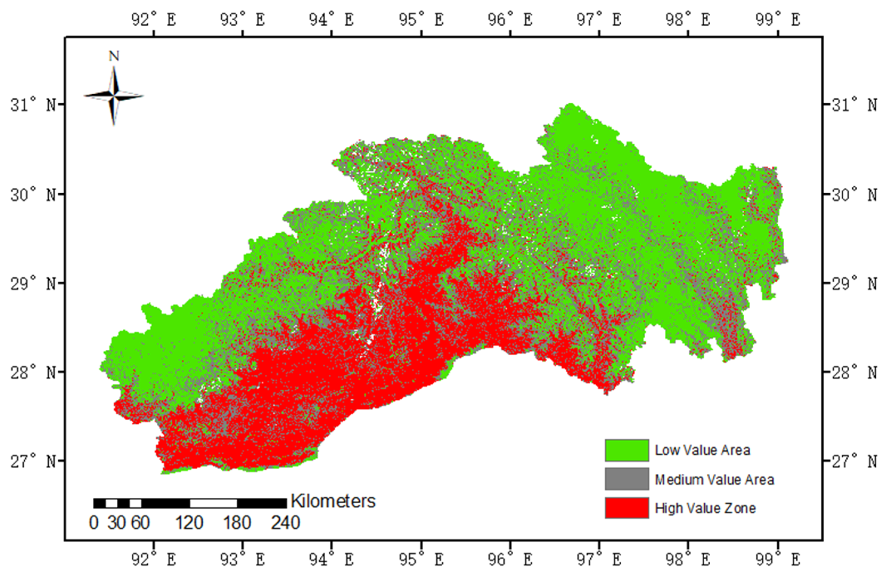
4.4. Spatial Variation in Carbon Stocks

To maximize the representation of the dynamic changes in carbon storage in southeastern Tibet, this study defines areas with an increase in raster carbon stock greater than 10 Mg/Ha from 2019 to 2023 as “growth areas”, and areas with a decrease below 10 Mg/Ha as “carbon reduction areas”. Regions with changes within ±10 Mg/Ha are classified as “areas with relatively stable carbon storage”, as illustrated in Figure 9.

From a spatial perspective, the variation in carbon storage exhibits distinct geographic distribution characteristics in southeastern Tibet. The blue areas in the figure represent areas of carbon loss, mainly concentrated in the central and southern parts of the map, indicating significant carbon loss in these areas from 2019 to 2023. In contrast, the red areas indicate areas of increased carbon, which are more sporadic but concentrated in certain regions in the west and east. The green areas represent regions where carbon stocks are relatively stable and are widely distributed in southeastern Tibet, indicating that the ecosystem in the region has remained relatively stable over the past few years with no significant changes in carbon stocks.

From a time perspective, the data presented in the figure reflect the trend of changes in carbon stocks from 2019 to 2023. In the past five years, the carbon increase and decrease areas were distributed evenly in the central, southwest, and southeast of southeastern Tibet, the changes in carbon stocks were similar to those in the regions with higher carbon stocks, and the vegetation was relatively vigorous. Generally speaking, the area with increased carbon storage (red) is larger than the area with decreased carbon storage (blue).

In addition, the map also reveals the effects of different elevations and landforms on the changes in carbon stocks in southeast Tibet. High-altitude regions, constrained by climatic conditions, face challenges in vegetation recovery, resulting in minimal carbon storage changes; in contrast, low-altitude areas, characterized by more frequent human activities, exhibit more significant variations in carbon storage.

In summary, the changes in carbon storage in southeastern Tibet from 2019 to 2023 demonstrate notable spatial heterogeneity and temporal trends. The area of carbon gain in southeastern Tibet exceeds that of carbon loss (Figure 9), ultimately leading to an upward trend in carbon storage.

Spatially, there is a clear regional disparity in carbon storage across southeastern Tibet. To address this phenomenon, this study analyzes the relationship between carbon stock distribution and changes. Given that the carbon storage per unit grid ranges from 2 Mg/Ha to 188 Mg/Ha, the research area is categorized into three zones using the Natural Breaks Classification (NBC): low-value zone (≤45 Mg/Ha), medium-value zone (45–122 Mg/Ha), and high-value zone (≥122 Mg/Ha). As illustrated in Figure 10, the green area represents the low-value zone, the gray area indicates the medium-value zone, and the red area denotes the high-value zone.

The carbon stock zoning map of the forest ecosystem in southeastern Tibet (Figure 10) shows that the low-value zone is primarily concentrated in the northwestern and northeastern parts of the region, where land use types predominantly consist of bare land and sparse vegetation, along with sporadic distributions in grasslands and moss-lichen areas characterized by low biomass and weak carbon sequestration capacity. The low carbon stock in these areas can be attributed to factors such as high elevation, cold climate, and poor soil conditions, which hinder vegetation growth, leading to lower biomass and, consequently, reduced carbon storage. Additionally, the low-value zone includes areas of bare land and sparse vegetation where low vegetation coverage precludes significant carbon accumulation.

The medium-value zone is mainly located near snow and ice surfaces and water bodies, exhibiting moderate to high carbon density and strong carbon sequestration potential. These areas benefit from relatively mild climatic conditions and suitable soil properties, promoting diverse plant growth, and resulting in intermediate carbon storage levels. The high-value zone is primarily situated in the southwestern part of southeastern Tibet, dominated by forest land use, characterized by high carbon density and robust carbon sequestration capacity. This region enjoys a warm and humid climate, abundant rainfall, and fertile soils that provide optimal conditions for forest growth, thereby further enhancing carbon storage.

From 2019 to 2023, the low-value zone in the study area remained relatively stable, the medium-value zone decreased, and the high-value zone increased (Figure 10), leading to a generally stable total carbon storage with minor fluctuations showing an increasing trend.

The total carbon storage of the forest ecosystem in Tibet is estimated at 1137.57 Tg, with the spatial distribution pattern of carbon storage revealing that the regions of Chamdo, Nyingchi, and Shannan possess relatively high carbon stocks, whereas the carbon storage in the forest ecosystems of Lhasa is comparatively lower.

4.5. Land Use Changes

This study analyzes land use based on 2020 data, categorizing various land types such as tree cover, shrub areas, grasslands, croplands, built-up areas, bare or sparse vegetation, snow and ice, permanent water bodies, and moss and lichen distributions, as shown in Figure 11.

The map indicates that tree cover is predominantly found in the southwest, with limited distribution in the north and east. Shrub areas are sparsely scattered in the northeast and west. Grasslands are widespread, particularly in the northwest and northeast, with some presence in the southeast. Croplands are mainly concentrated in the southwestern boundaries, with minimal central distribution. Built-up areas are the least common, appearing sporadically across southeastern Tibet. Bare or sparse vegetation shares a similar distribution pattern with grasslands but covers a smaller area. Snow and ice are found on the region’s peaks, while permanent water bodies are limited to the northwest, southwest, and eastern boundaries. Moss and lichen are widely distributed, except for some areas in the southwest and east.

The changes in land use types from 2019 to 2023 were analyzed and depicted in Figure 12. Overall, the distribution pattern remained relatively stable, but notable changes include an increase in tree cover, particularly in the southwest and central areas, reflecting effective vegetation recovery and forest management. Conversely, grasslands and bare areas decreased, possibly transitioning to tree cover or shrub areas. The changes in cropland and built-up areas were minimal, though some cropland increased locally, potentially linked to agricultural development. Permanent water bodies remained stable, with some seasonal fluctuations in certain river and lake areas.

Table 4. Land use types and carbon stocks in Southeast Tibet, 2019~2023.

Date	Tree Cover Area (Mg/Ha)	Grassland (Mg/Ha)	Bare Land (Mg/Ha)		Moss and Lichen (Mg/Ha)
2019/4~6	10,825,898.18	1,972,312.96	639,020.41		1,538,898.73
2019/7~9	10,836,024.28	2,028,491.50	659,046.16		1,545,958.08
2019/10~12	10,779,628.60	1,950,861.47	637,115.40		1,547,470.50
2020/1~3	10,751,296.34	1,968,002.20	655,532.41		1,557,478.03
2020/4~6	10,793,722.44	1,974,786.93	645,823.47		1,521,998.26
2020/7~9	10,685,850.11	2,052,525.26	685,247.47		1,543,250.54
2020/10~12	10,795,310.15	1,938,352.72	646,086.74		1,541,154.79
2021/1~3	10,784,374.29	1,908,254.81	650,782.27		1,536,230.22
2021/4~6	10,739,138.49	1,968,437.78	651,443.55		1,532,525.53
2021/7~9	10,776,819.99	2,042,477.70	661,259.31		1,526,887.50
2021/10~12	10,045,654.35	1,739,061.64	462,868.64		1,108,598.84
2022/1~3	8,117,408.88	1,489,891.11	491,115.50		966,456.92
2022/4~6	5,807,508.51	906,253.94	337,180.44		498,248.04
2022/7~9	6,894,336.98	1,299,965.37	385,925.06		607,655.09
2022/10~12	10,730,775.92	1,844,725.16	598,387.25		1,316,321.50
2023/1~3	8,841,339.32	1,744,769.52	600,574.40		1,171,694.32
2023/4~6	8,495,046.30	1,593,904.99	524,725.60		982,088.93
2023/7~9	6,213,510.85	1,343,282.32	387,227.06		578,449.27
2023/10~12	10,773,944.01	1,808,503.07	598,995.93		1,340,219.02
Date	Snow-Covered Areas (Mg/Ha)	Shrubland (Mg/Ha)	Farmland (Mg/Ha)	Built-Up Area (Mg/Ha)	Permanent Water (Mg/Ha)
2019/4~6	703,445.72	6046.24	37,387.52	3518.67	62,796.85
2019/7~9	668,936.29	6963.55	38,506.11	3468.91	61,909.22
2019/10~12	714,548.49	6130.38	36,454.05	3706.50	62,397.53
2020/1~3	753,682.68	6543.10	35,240.09	3458.08	61,926.03
2020/4~6	717,491.04	6618.97	35,612.61	3485.54	62,251.26
2020/7~9	682,566.72	6961.82	36,959.43	3376.23	61,803.60
2020/10~12	729,120.88	5660.19	35,201.45	3550.20	63,215.65
2021/1~3	730,086.59	5734.89	36,746.34	3546.28	63,412.09
2021/4~6	713,226.60	6130.17	36,928.61	3416.25	62,386.24
2021/7~9	662,958.56	6954.65	35,135.31	3253.16	60,588.88
2021/10~12	536,588.79	6343.45	32,646.99	3290.38	58,045.72
2022/1~3	454,250.07	5867.88	31,028.18	3031.34	46,440.98
2022/4~6	319,116.52	5451.07	35,317.23	3238.56	45,695.64
2022/7~9	238,724.06	6378.60	34,595.27	3158.64	50,806.85
2022/10~12	631,592.36	6434.82	32,733.08	3194.29	61,124.07
2023/1~3	585,326.12	6300.34	31,620.93	2921.51	53,606.08
2023/4~6	524,245.37	5749.91	33,968.21	3509.65	58,456.56
2023/7~9	167,647.70	5911.59	33,426.22	2650.58	43,115.36
2023/10~12	651,446.08	6511.22	34,482.96	3274.17	63,124.31

provides a detailed overview of aboveground carbon stocks for different land use types in Mg. The data reveals that from 2019 to 2023, tree cover played a crucial role in carbon storage, accounting for over half of the total carbon stock in the region. Grasslands along with moss and lichen maintained a stable share of around 22% of total carbon stocks, indicating consistent development without significant fluctuations. In contrast, bare or sparse vegetation, snow, and ice contributed approximately 4%, with bare areas slightly lower than snow and ice. Croplands and permanent water bodies consistently accounted for about 0.6% of total carbon stocks, with temporary increases during harvest seasons in 2022 and 2023. Finally, built-up and shrub areas had the smallest contributions, so negligible that they can be disregarded.

As shown in Table 4 and Figure 13, the carbon density in the southeastern Tibet region remained relatively stable with slight periodic fluctuations from 2019 to 2023, correlating with seasonal variations. The average carbon density was 74.43 Mg/Ha, and during these five years, the carbon density consistently hovered around 75 Mg/Ha. Overall, the carbon densities in shrub areas, grasslands, agricultural lands, built-up areas, bare or sparse vegetation, snow and ice surfaces, permanent water bodies, mosses, and lichens remained relatively stable.

The tree cover area experienced an increase, with its proportion rising from 68.49% to 70.50%, representing a 2.01% increase. Permanent water bodies also saw a slight increase, with their proportion rising from 0.396% to 0.413%, an increase of 0.017%. The proportions of shrub areas, agricultural lands, and built-up areas remained largely unchanged, with variations within 0.01%. Grassland areas decreased, with their proportion dropping from 12.40% to 11.84%, a decline of 0.66%. Additionally, bare or sparse vegetation decreased from 4.05% to 3.92%, a decline of 0.13%. Snow and ice surfaces also saw a reduction, from 4.54% to 4.26%, a decrease of 0.28%, while the proportion of mosses and lichens decreased from 9.83% to 8.77%, a decline of 1.06%. Collectively, the proportions of grasslands, bare or sparse vegetation, snow and ice surfaces, and mosses and lichens decreased from 30.816% to 28.789%, a decline of 2.027%. In contrast, the combined proportions of tree cover and permanent water bodies increased from 68.889% to 70.921%, an increase of 2.032%. The increase in proportion exceeds the decrease, indicating an overall upward trend in carbon density in the southeastern Tibet region.

Over the past five years, the overall carbon stock in the southeastern Tibet region has shown a fluctuating increasing trend. Land use changes are one of the key factors contributing to variations in ecosystem carbon stocks. The transition in land cover types in Tibet has enhanced carbon accumulation functionality. The area of carbon-dense classes, such as tree cover and permanent water bodies, has increased, while the area of carbon-poor classes, such as grasslands, bare or sparse vegetation, snow and ice surfaces, and mosses and lichens, has decreased. Adjusting land use structure and increasing the area of high carbon density grade can effectively improve carbon accumulation capacity.

The main land use types in southeast Tibet are forest cover and grassland, and the increase in forest cover is the main reason for the increase of carbon storage. Thus, changes in land use patterns, especially from grassland to forest cover, highlight the importance of sound land management and ecological restoration measures in improving regional carbon stocks and carbon sequestration capacity.

The effects of land use factors on the spatial pattern of forest carbon storage in southeast Tibet were mainly reflected in the changes in land use types and the effects of elevation gradient on soil organic carbon and microbial communities. Through rational adjustment of land use structure and protection and restoration of natural vegetation, regional carbon sequestration capacity can be effectively enhanced, which is crucial to addressing global climate change.

4.6. Impact Factor Analysis

The study selected factors influencing carbon storage from ERA5 and SRTM datasets. After completing model training, we retrospectively examined the training process to analyze the role of each factor in constructing decision trees and their contributions to reducing prediction errors through quantitative analysis. This research utilized data from March to June 2020 to investigate these factors. This period encompasses spring and early summer, which is a critical phase for vegetation growth. During this time, vegetation transitions from winter dormancy to active metabolism, making it a key window for capturing forest structure parameters.

The influencing factors for carbon stocks are presented in

Table 5. Variables and importance score.

Features	Importance Score
elevation	22.06
slope	17.00
temperature	22.04
precipitation	9.57
surface pressure	16.79
east–west wind speed	8.53
north–south wind speed	4.02

. Table 5 displays the scores for each factor. The score for elevation is 22.06, for slope it is 17.00, for temperature it is 22.04, for precipitation it is 9.57, for surface pressure it is 16.79, for east–west wind speed it is 8.53, and for north–south wind speed it is 4.02. The factors are ranked from highest to lowest as follows: elevation, temperature, slope, surface pressure, precipitation, east–west wind speed, and north–south wind speed.

5. Discussion

This study employs multi-source remote sensing data and advanced classification and change detection techniques to provide an effective method for assessing land cover changes in national nature reserves and forest parks. Remote sensing technology offers high temporal and spatial resolution continuous observation data, addressing the limitations of traditional surveys [39,40]. The application of machine learning algorithms further enhances classification accuracy and sensitivity in change detection [41]. However, remote sensing monitoring faces challenges, such as the need for reliable imputation methods to address cloud cover interference [42,43].

In addition, the internal heterogeneity of protected areas makes it difficult to determine specific ecological conditions based on remote sensing alone [44]; therefore, an integrated analysis of integrated field survey data is necessary.

5.1. Advantages of the Research Techniques

The Google Earth Engine (GEE) platform has powerful data processing and analysis capabilities to integrate remote sensing data, GIS data, and field survey data [45,46]. This integration is critical for analyzing the complex impacts of topography, climate, and land use changes on carbon stocks in southeastern Xizang. Due to its unique geographical location and variable climatic conditions, the factors affecting soil organic carbon pools are complex and require efficient data processing tools for accurate analysis. The GEE platform not only supports the integration of multidisciplinary data and methods but also provides a variety of spatial analysis tools, such as the Moran’s I index and high/low cluster analysis [47,48]. These tools help identify spatial distribution patterns and trends of soil organic carbon stocks and clarify their relationship with environmental factors. In addition, the powerful real-time visualization capabilities of the GEE platform enable researchers to visually observe temporal and spatial changes in carbon stocks [49,50]. In general, the GEE platform provides a valuable technical tool for the in-depth study of soil organic carbon reserves in southeast Tibet.

These advantages are further enhanced by the integration of multi-sensor data. Sentinel-1’s all-weather capability supplements optical data under cloud coverage conditions, while GEDI’s vertical structure detection optimizes biomass estimation in dense forest areas. Combined with the efficient data processing capability of the gradient enhancement algorithm, this study realizes collaborative analysis of multi-source remote sensing data, significantly improving the accuracy of carbon storage prediction (validation set R² = 0.909, RMSE = 26.608 Mg/Ha), which is better than the method that relies on a single sensor. In addition, automated feature extraction reduces manual operations, allowing it to be efficiently applied to large-scale monitoring of complex terrains.

5.2. Drivers of Spatiotemporal Carbon Dynamics

The data (Figure 8) suggest that carbon density exhibits periodic fluctuations over time, possibly linked to seasonal changes affecting vegetation growth and carbon storage capacity [51,52,53]. From 2019 to 2020, a slight upward trend indicates the potential for increased carbon storage due to natural growth or human intervention. The notable changes in the area suggest that factors beyond seasonal variation, including human activities such as land use changes and forestry management, significantly influence these dynamics [54,55,56].

The spatial analysis in Section 4.4 shows that the carbon loss areas (green) in the central and southern regions may be caused by deforestation, land use change, or natural disasters [57]. On the contrary, the carbon storage in scattered areas (red) in the west and east increased, indicating that there may be vegetation restoration, improvement of forest management measures, or other activities to increase carbon storage in these areas which contributed to the trend of the regional carbon gain area exceeding the loss area [58,59].

The phenomenon of carbon loss in the blue (Figure 9) areas warrants attention, as it may negatively impact the regional ecological environment and contribute to climate change [60]. The increase in carbon storage in the red (Figure 9) areas indicates some success in ecological restoration measures in specific locations [61,62,63]. Moving forward, it is essential to enhance forest protection, land management, and ecological restoration efforts to mitigate carbon loss, augment carbon storage, and achieve sustainable development in the region [64,65,66].

The area of the region with increased carbon reserves in southeast Tibet is larger than the area with decreased carbon reserves, and the region generally shows a trend of increasing carbon. This trend may be related to the increase in human activities, the impact of climate change, and the degradation of ecosystems [67,68,69].

The carbon density fluctuations observed in this study need to be explained in conjunction with the uncertainty of remote sensing data. Firstly, the fusion of optical and radar data may introduce systematic biases due to differences in phase and resolution. Secondly, incomplete terrain correction or residual cloud shadows may lead to local inversion errors. Finally, the insufficient sensitivity of the model to vegetation parameters in high-altitude regions may limit the accuracy of inversion. Despite these limitations, the long-term upward trend of carbon density is still consistent with the driving effect of forest expansion, indicating its ecological significance.

5.3. Effects of National Nature Reserve and Forest Park Policies

The Tibet Autonomous Region is rich in forest resources and carbon reserves, playing an important role in tackling climate change [70]. Globally, forests are among the largest carbon reservoirs and are crucial for regulating climate and absorbing atmospheric carbon dioxide [71].

Natural reserves contribute significantly to the increase in carbon stocks. Research indicates a rising trend in carbon stocks in the natural reserves of the Tibetan Plateau from 2000 to 2015, consistent with the role of forests as important carbon sinks worldwide, wherein they regulate atmospheric carbon dioxide levels through carbon fixation and oxygen release.

The policies surrounding natural reserves enhance ecological environment quality through the implementation of ecological protection and restoration projects. For example, the ecological quality of the Sanjiangyuan region has significantly improved following the enactment of natural reserve policies, with unused land being converted into ecological land, thus enhancing environmental quality [72].

Land cover type shifts have augmented carbon sequestration functionality, contributing 269% to the changes in carbon accumulation. This underscores that effective planning and management, such as establishing forest parks, can significantly promote the transition of land cover to higher carbon density classes, thereby increasing carbon stocks.

National forest parks play a crucial role in mitigating climate change and maintaining carbon balance [73], with average carbon densities surpassing the national average for forest ecosystems, contributing 11.0% to 12.2% of the total carbon stocks in China’s forest ecosystems. This indicates a positive impact of forest parks on carbon stocks and sequestration rates within regional forest ecosystems.

Globally, forests act as significant carbon sinks, capable of absorbing atmospheric carbon dioxide. In China, forest ecosystems demonstrate carbon sink characteristics in gas exchange with the atmosphere, with an annual flux of approximately 4.80 × 10⁸ t·a⁻¹. Therefore, establishing forest parks not only enhances carbon stocks within regions but also positively influences global carbon cycling [74].

Consequently, the establishment of natural reserves and national forest parks is particularly vital. Research indicates that, under future climatic scenarios, optimizing the planning of natural reserves can effectively identify and protect regions that are relatively stable in terms of climate, thereby maintaining or enhancing ecosystem services and carbon stocks [75].

5.4. Comparison with Existing Research

Compared with studies that rely solely on optical remote sensing (such as Landsat), this study improves the characterization ability of forest vertical structures by fusing SAR (Sentinel-1) and LiDAR (GEDI) data [32]. However, spatial resolution limits of LiDAR data may still affect the detection of local heterogeneity, which is consistent with the conclusions of similar multi-source data fusion studies.

The upward trend of carbon reserves in this study is consistent with the studies of other plateau forest ecosystems, but the interannual fluctuation amplitude is smaller than that of tropical rainforests. This may reflect the stability of mature forests and the effectiveness of regional conservation policies [22].

The positive correlation between the expansion of forest coverage and the increase in carbon reserves supports the effectiveness of protected areas policies, which is consistent with similar research results of the Qinghai–Tibet Plateau National Park System [21].

6. Conclusions

This study is based on the Google Earth Engine (GEE) platform, integrating multi-source remote sensing data (Landsat 8, Sentinel-1, GEDI), and systematically analyzes the spatiotemporal changes in carbon reserves of primeval forests in southeastern Tibet from 2019 to 2023. By systematically evaluating a variety of machine learning algorithms (including Random Forests, CART, Support Vector Machines, and Gradient Boosting), the results show that the Gradient Boosting algorithm exhibits optimal performance in characterizing the spatiotemporal dynamics of carbon storage. The results demonstrate that the Gradient Boosting algorithm exhibits significant advantages in characterizing the spatiotemporal dynamics of carbon storage. The study reveals an overall fluctuating upward trend in carbon stocks, with noticeable improvements in average carbon density and distinct interannual variations. This growth is primarily associated with the expansion of forest restoration and regeneration areas. Spatially, the increase in carbon storage is predominantly concentrated in the central and southern regions of the study area. It should be emphasized that the multi-source nature of remote sensing data and model inversion errors may have a certain impact on carbon density estimation, such as data loss caused by cloud coverage or inherent sensor errors. However, the stability of long-term trends is consistent with the ecological process of land use transformation, supporting its policy reference value. In the future, the reliability of the results needs to be further verified through ground measurements and high-resolution sensors.

The change in carbon storage in southeastern Tibet is affected by many factors, such as temperature, precipitation, elevation, slope, land use change, and human activities. These factors interact through complex mechanisms, resulting in significant spatiotemporal changes in carbon stocks. The potential effects of land use change on carbon stocks were further investigated. The study found that the loss of grassland and bare land, combined with the increase in tree cover, had a significant, positive effect on carbon accumulation. These land use changes not only enhance regional carbon sink functions but also contribute to climate change mitigation. Therefore, rational land use planning is an effective way to increase regional carbon storage and reduce greenhouse gas emissions.

References

1. Yu, C.; Zhang, Y.; Claus, H.; Zeng, R.; Zhang, X.; Wang, J. Ecological and Environmental Issues Faced by a Developing Tibet. Environ. Sci. Technol. 2012, 46, 1979–1980. [Google Scholar] [CrossRef]
2. Zhao, D.; Wu, S.; Yin, Y.; Yin, Z.-Y. Vegetation Distribution on Tibetan Plateau under Climate Change Scenario. Reg. Environ. Chang. 2011, 11, 905–915. [Google Scholar] [CrossRef]
3. Shen, W.; Zhang, L.; Luo, T. Causes for the Increase of Early-Season Freezing Events under a Warmer Climate at Alpine Treelines in Southeast Tibet. Agric. For. Meteorol. 2022, 316, 108863. [Google Scholar] [CrossRef]
4. Zu, K.; Wang, Z.; Zhu, X.; Lenoir, J.; Shrestha, N.; Lyu, T.; Luo, A.; Li, Y.; Ji, C.; Peng, S.; et al. Upward Shift and Elevational Range Contractions of Subtropical Mountain Plants in Response to Climate Change. Sci. Total Environ. 2021, 783, 146896. [Google Scholar] [CrossRef]
5. Sun, W.; Liu, X. Review on Carbon Storage Estimation of Forest Ecosystem and Applications in China. For. Ecosyst. 2019, 7, 4. [Google Scholar] [CrossRef]
6. Zeng, W.-S. Development of Monitoring and Assessment of Forest Biomass and Carbon Storage in China. For. Ecosyst. 2014, 1, 20. [Google Scholar] [CrossRef]
7. Tian, L.; Wu, X.; Tao, Y.; Li, M.; Qian, C.; Liao, L.; Fu, W. Review of Remote Sensing-Based Methods for Forest Aboveground Biomass Estimation: Progress, Challenges, and Prospects. Forests 2023, 14, 1086. [Google Scholar] [CrossRef]
8. Pham, T.D.; Yokoya, N.; Bui, D.T.; Yoshino, K.; Friess, D.A. Remote Sensing Approaches for Monitoring Mangrove Species, Structure, and Biomass: Opportunities and Challenges. Remote Sens. 2019, 11, 230. [Google Scholar] [CrossRef]
9. Lu, D.; Chen, Q.; Wang, G.; Liu, L.; Li, G.; Moran, E. A Survey of Remote Sensing-Based Aboveground Biomass Estimation Methods in Forest Ecosystems. Int. J. Digit. Earth 2016, 9, 63–105. [Google Scholar] [CrossRef]
10. Drake, J.B.; Dubayah, R.O.; Clark, D.B.; Knox, R.G.; Blair, J.B.; Hofton, M.A.; Chazdon, R.L.; Weishampel, J.F.; Prince, S. Estimation of Tropical Forest Structural Characteristics Using Large-Footprint Lidar. Remote Sens. Environ. 2002, 79, 305–319. [Google Scholar] [CrossRef]
11. Zimble, D.A.; Evans, D.L.; Carlson, G.C.; Parker, R.C.; Grado, S.C.; Gerard, P.D. Characterizing Vertical Forest Structure Using Small-Footprint Airborne LiDAR. Remote Sens. Environ. 2003, 87, 171–182. [Google Scholar] [CrossRef]
12. Safari, A.; Sohrabi, H. Integration of Synthetic Aperture Radar and Multispectral Data for Aboveground Biomass Retrieval in Zagros Oak Forests, Iran: An Attempt on Sentinel Imagery. Int. J. Remote Sens. 2020, 41, 8069–8095. [Google Scholar] [CrossRef]
13. Treuhaft, R.N.; Law, B.E.; Asner, G.P. Forest Attributes from Radar Interferometric Structure and Its Fusion with Optical Remote Sensing. BioScience 2004, 54, 561–571. [Google Scholar] [CrossRef]
14. Kahraman, S.; Bacher, R. A Comprehensive Review of Hyperspectral Data Fusion with Lidar and Sar Data. Annu. Rev. Control 2021, 51, 236–253. [Google Scholar] [CrossRef]
15. Moghaddam, M.; Dungan, J.L.; Acker, S. Forest Variable Estimation from Fusion of SAR and Multispectral Optical Data. IEEE Trans. Geosci. Remote Sens. 2002, 40, 2176–2187. [Google Scholar] [CrossRef]
16. Liu, Z.; Peng, C.; Work, T.; Candau, J.-N.; DesRochers, A.; Kneeshaw, D. Application of Machine-Learning Methods in Forest Ecology: Recent Progress and Future Challenges. Environ. Rev. 2018, 26, 339–350. [Google Scholar] [CrossRef]
17. Zhao, Q.; Yu, S.; Zhao, F.; Tian, L.; Zhao, Z. Comparison of Machine Learning Algorithms for Forest Parameter Estimations and Application for Forest Quality Assessments. For. Ecol. Manag. 2019, 434, 224–234. [Google Scholar] [CrossRef]
18. Maxwell, A.E.; Warner, T.A.; Fang, F. Implementation of Machine-Learning Classification in Remote Sensing: An Applied Review. Int. J. Remote Sens. 2018, 39, 2784–2817. [Google Scholar] [CrossRef]
19. Jahromi, M.N.; Jahromi, M.N.; Zolghadr-Asli, B.; Pourghasemi, H.R.; Alavipanah, S.K. Google Earth Engine and Its Application in Forest Sciences. In Spatial Modeling in Forest Resources Management: Rural Livelihood and Sustainable Development; Shit, P.K., Pourghasemi, H.R., Das, P., Bhunia, G.S., Eds.; Springer International Publishing: Cham, Switzerland, 2021; pp. 629–649. ISBN 978-3-030-56542-8. [Google Scholar]
20. Liu, L.; Guo, Y.; Li, Y.; Zhang, Q.; Li, Z.; Chen, E.; Yang, L.; Mu, X. Comparison of Machine Learning Methods Applied on Multi-Source Medium-Resolution Satellite Images for Chinese Pine (Pinus tabulaeformis) Extraction on Google Earth Engine. Forests 2022, 13, 677. [Google Scholar] [CrossRef]
21. Zhao, L.; Du, M.; Du, W.; Guo, J.; Liao, Z.; Kang, X.; Liu, Q. Evaluation of the Carbon Sink Capacity of the Proposed Kunlun Mountain National Park. Int. J. Environ. Res. Public Health 2022, 19, 9887. [Google Scholar] [CrossRef]
22. Sun, X.; Wang, G.; Huang, M.; Chang, R.; Ran, F. Forest Biomass Carbon Stocks and Variation in Tibet’s Carbon-Dense Forests from 2001 to 2050. Sci. Rep. 2016, 6, 34687. [Google Scholar] [CrossRef] [PubMed]
23. Xu, H.; Yue, C.; Zhang, Y.; Liu, D.; Piao, S. Forestation at the Right Time with the Right Species Can Generate Persistent Carbon Benefits in China. Proc. Natl. Acad. Sci. USA 2023, 120, e2304988120. [Google Scholar] [CrossRef] [PubMed]
24. Liang, E.; Wang, Y.; Eckstein, D.; Luo, T. Little Change in the Fir Tree-Line Position on the Southeastern Tibetan Plateau after 200 Years of Warming. New Phytol. 2011, 190, 760–769. [Google Scholar] [CrossRef] [PubMed]
25. Zhou, L.; Zhu, J.; Zou, H.; Ma, S.; Li, P.; Zhang, Y.; Huo, C. Atmospheric Moisture Distribution and Transport over the Tibetan Plateau and the Impacts of the South Asian Summer Monsoon. Acta Meteorol. Sin. 2013, 27, 819–831. [Google Scholar] [CrossRef]
26. Keyimu, M.; Li, Z.; Liu, G.; Fu, B.; Fan, Z.; Wang, X.; Wu, X.; Zhang, Y.; Halik, U. Tree-Ring Based Minimum Temperature Reconstruction on the Southeastern Tibetan Plateau. Quat. Sci. Rev. 2021, 251, 106712. [Google Scholar] [CrossRef]
27. Shi, S.; Liu, G.; Li, Z.; Ye, X. Elevation-Dependent Growth Trends of Forests as Affected by Climate Warming in the Southeastern Tibetan Plateau. For. Ecol. Manag. 2021, 498, 119551. [Google Scholar] [CrossRef]
28. Kuang, X.; Jiao, J.J. Review on Climate Change on the Tibetan Plateau during the Last Half Century. J. Geophys. Res. Atmos. 2016, 121, 3979–4007. [Google Scholar] [CrossRef]
29. Roy, D.P.; Wulder, M.A.; Loveland, T.R.; Woodcock, C.E.; Allen, R.G.; Anderson, M.C.; Helder, D.; Irons, J.R.; Johnson, D.M.; Kennedy, R. Landsat-8: Science and Product Vision for Terrestrial Global Change Research. Remote Sens. Environ. 2014, 145, 154–172. [Google Scholar] [CrossRef]
30. Rüetschi, M.; Schaepman, M.E.; Small, D. Using Multitemporal Sentinel-1 C-Band Backscatter to Monitor Phenology and Classify Deciduous and Coniferous Forests in Northern Switzerland. Remote Sens. 2018, 10, 55. [Google Scholar] [CrossRef]
31. Lehmann, E.A.; Caccetta, P.; Lowell, K.; Mitchell, A.; Zhou, Z.-S.; Held, A.; Milne, T.; Tapley, I. SAR and Optical Remote Sensing: Assessment of Complementarity and Interoperability in the Context of a Large-Scale Operational Forest Monitoring System. Remote Sens. Environ. 2015, 156, 335–348. [Google Scholar] [CrossRef]
32. Schneider, F.D.; Ferraz, A.; Hancock, S.; Duncanson, L.I.; Dubayah, R.O.; Pavlick, R.P.; Schimel, D.S. Towards Mapping the Diversity of Canopy Structure from Space with GEDI. Environ. Res. Lett. 2020, 15, 115006. [Google Scholar] [CrossRef]
33. Qi, W.; Saarela, S.; Armston, J.; Ståhl, G.; Dubayah, R. Forest Biomass Estimation over Three Distinct Forest Types Using TanDEM-X InSAR Data and Simulated GEDI Lidar Data. Remote Sens. Environ. 2019, 232, 111283. [Google Scholar] [CrossRef]
34. Belgiu, M.; Drăguţ, L. Random Forest in Remote Sensing: A Review of Applications and Future Directions. ISPRS J. Photogramm. Remote Sens. 2016, 114, 24–31. [Google Scholar] [CrossRef]
35. Loh, W.-Y. Classification and Regression Trees. WIREs Data Min. Knowl. Discov. 2011, 1, 14–23. [Google Scholar] [CrossRef]
36. Chicco, D.; Warrens, M.J.; Jurman, G. The Coefficient of Determination R-Squared Is More Informative than SMAPE, MAE, MAPE, MSE and RMSE in Regression Analysis Evaluation. PeerJ Comput. Sci. 2021, 7, e623. [Google Scholar] [CrossRef]
37. Petersson, H.; Holm, S.; Ståhl, G.; Alger, D.; Fridman, J.; Lehtonen, A.; Lundström, A.; Mäkipää, R. Individual Tree Biomass Equations or Biomass Expansion Factors for Assessment of Carbon Stock Changes in Living Biomass—A Comparative Study. For. Ecol. Manag. 2012, 270, 78–84. [Google Scholar] [CrossRef]
38. Guo, Z.; Fang, J.; Pan, Y.; Birdsey, R. Inventory-Based Estimates of Forest Biomass Carbon Stocks in China: A Comparison of Three Methods. For. Ecol. Manag. 2010, 259, 1225–1231. [Google Scholar] [CrossRef]
39. Wang, K.; Franklin, S.E.; Guo, X.; Cattet, M. Remote Sensing of Ecology, Biodiversity and Conservation: A Review from the Perspective of Remote Sensing Specialists. Sensors 2010, 10, 9647–9667. [Google Scholar] [CrossRef]
40. Ma, Y.; Wu, H.; Wang, L.; Huang, B.; Ranjan, R.; Zomaya, A.; Jie, W. Remote Sensing Big Data Computing: Challenges and Opportunities. Future Gener. Comput. Syst. 2015, 51, 47–60. [Google Scholar] [CrossRef]
41. Goswami, A.; Sharma, D.; Mathuku, H.; Gangadharan, S.M.P.; Yadav, C.S.; Sahu, S.K.; Pradhan, M.K.; Singh, J.; Imran, H. Change Detection in Remote Sensing Image Data Comparing Algebraic and Machine Learning Methods. Electronics 2022, 11, 431. [Google Scholar] [CrossRef]
42. Fassnacht, F.E.; White, J.C.; Wulder, M.A.; Næsset, E. Remote Sensing in Forestry: Current Challenges, Considerations and Directions. For. Int. J. For. Res. 2024, 97, 11–37. [Google Scholar] [CrossRef]
43. Nazarova, T.; Martin, P.; Giuliani, G. Monitoring Vegetation Change in the Presence of High Cloud Cover with Sentinel-2 in a Lowland Tropical Forest Region in Brazil. Remote Sens. 2020, 12, 1829. [Google Scholar] [CrossRef]
44. Nagendra, H.; Lucas, R.; Honrado, J.P.; Jongman, R.H.G.; Tarantino, C.; Adamo, M.; Mairota, P. Remote Sensing for Conservation Monitoring: Assessing Protected Areas, Habitat Extent, Habitat Condition, Species Diversity, and Threats. Ecol. Indic. 2013, 33, 45–59. [Google Scholar] [CrossRef]
45. Amani, M.; Ghorbanian, A.; Ahmadi, S.A.; Kakooei, M.; Moghimi, A.; Mirmazloumi, S.M.; Moghaddam, S.H.A.; Mahdavi, S.; Ghahremanloo, M.; Parsian, S.; et al. Google Earth Engine Cloud Computing Platform for Remote Sensing Big Data Applications: A Comprehensive Review. IEEE J. Sel. Top. Appl. Earth Obs. Remote Sens. 2020, 13, 5326–5350. [Google Scholar] [CrossRef]
46. Tamiminia, H.; Salehi, B.; Mahdianpari, M.; Quackenbush, L.; Adeli, S.; Brisco, B. Google Earth Engine for Geo-Big Data Applications: A Meta-Analysis and Systematic Review. ISPRS J. Photogramm. Remote Sens. 2020, 164, 152–170. [Google Scholar] [CrossRef]
47. Zhao, Z.; Li, T.; Zhang, Y.; Lü, D.; Wang, C.; Lü, Y.; Wu, X. Spatiotemporal Patterns and Driving Factors of Ecological Vulnerability on the Qinghai-Tibet Plateau Based on the Google Earth Engine. Remote Sens. 2022, 14, 5279. [Google Scholar] [CrossRef]
48. Liu, C.; Li, W.; Wang, W.; Zhou, H.; Liang, T.; Hou, F.; Xu, J.; Xue, P. Quantitative Spatial Analysis of Vegetation Dynamics and Potential Driving Factors in a Typical Alpine Region on the Northeastern Tibetan Plateau Using the Google Earth Engine. CATENA 2021, 206, 105500. [Google Scholar] [CrossRef]
49. Cheng, F.; Ou, G.; Wang, M.; Liu, C. Remote Sensing Estimation of Forest Carbon Stock Based on Machine Learning Algorithms. Forests 2024, 15, 681. [Google Scholar] [CrossRef]
50. Zhang, X.; Jia, W.; Sun, Y.; Wang, F.; Miu, Y. Simulation of Spatial and Temporal Distribution of Forest Carbon Stocks in Long Time Series—Based on Remote Sensing and Deep Learning. Forests 2023, 14, 483. [Google Scholar] [CrossRef]
51. Klumpp, K.; Tallec, T.; Guix, N.; Soussana, J.-F. Long-Term Impacts of Agricultural Practices and Climatic Variability on Carbon Storage in a Permanent Pasture. Glob. Change Biol. 2011, 17, 3534–3545. [Google Scholar] [CrossRef]
52. Post, W.M.; Kwon, K.C. Soil Carbon Sequestration and Land-Use Change: Processes and Potential. Glob. Change Biol. 2000, 6, 317–327. [Google Scholar] [CrossRef]
53. Emanuel, W.R.; Killough, G.G. Modeling Terrestrial Ecosystems in the Global Carbon Cycle with Shifts in Carbon Storage Capacity by Land-Use Change. Ecology 1984, 65, 970–983. [Google Scholar] [CrossRef]
54. Birdsey, R.; Pan, Y. Trends in Management of the World’s Forests and Impacts on Carbon Stocks. For. Ecol. Manag. 2015, 355, 83–90. [Google Scholar] [CrossRef]
55. Dale, V.H. The Relationship Between Land-Use Change and Climate Change. Ecol. Appl. 1997, 7, 753–769. [Google Scholar] [CrossRef]
56. Jandl, R.; Lindner, M.; Vesterdal, L.; Bauwens, B.; Baritz, R.; Hagedorn, F.; Johnson, D.W.; Minkkinen, K.; Byrne, K.A. How Strongly Can Forest Management Influence Soil Carbon Sequestration? Geoderma 2007, 137, 253–268. [Google Scholar] [CrossRef]
57. Sy, V.D.; Herold, M.; Achard, F.; Beuchle, R.; Clevers, J.G.P.W.; Lindquist, E.; Verchot, L. Land Use Patterns and Related Carbon Losses Following Deforestation in South America. Environ. Res. Lett. 2015, 10, 124004. [Google Scholar] [CrossRef]
58. Houghton, R.A.; House, J.I.; Pongratz, J.; van der Werf, G.R.; DeFries, R.S.; Hansen, M.C.; Le Quéré, C.; Ramankutty, N. Carbon Emissions from Land Use and Land-Cover Change. Biogeosciences 2012, 9, 5125–5142. [Google Scholar] [CrossRef]
59. Gatti, L.V.; Basso, L.S.; Miller, J.B.; Gloor, M.; Gatti Domingues, L.; Cassol, H.L.G.; Tejada, G.; Aragão, L.E.O.C.; Nobre, C.; Peters, W.; et al. Amazonia as a Carbon Source Linked to Deforestation and Climate Change. Nature 2021, 595, 388–393. [Google Scholar] [CrossRef]
60. White, A.; Cannell, M.G.R.; Friend, A.D. Climate Change Impacts on Ecosystems and the Terrestrial Carbon Sink: A New Assessment. Glob. Environ. Chang. 1999, 9, S21–S30. [Google Scholar] [CrossRef]
61. Bernal, B.; Murray, L.T.; Pearson, T.R.H. Global Carbon Dioxide Removal Rates from Forest Landscape Restoration Activities. Carbon Balance Manag. 2018, 13, 22. [Google Scholar] [CrossRef]
62. Gann, G.D.; McDonald, T.; Walder, B.; Aronson, J.; Nelson, C.R.; Jonson, J.; Hallett, J.G.; Eisenberg, C.; Guariguata, M.R.; Liu, J.; et al. International Principles and Standards for the Practice of Ecological Restoration. Restor. Ecol. 2019, 27, S1–S46. [Google Scholar] [CrossRef]
63. Suding, K.N. Toward an Era of Restoration in Ecology: Successes, Failures, and Opportunities Ahead. Annu. Rev. Ecol. Evol. Syst. 2011, 42, 465–487. [Google Scholar] [CrossRef]
64. Ciccarese, L.; Mattsson, A.; Pettenella, D. Ecosystem Services from Forest Restoration: Thinking Ahead. New For. 2012, 43, 543–560. [Google Scholar] [CrossRef]
65. Bustamante, M.M.C.; Silva, J.S.; Scariot, A.; Sampaio, A.B.; Mascia, D.L.; Garcia, E.; Sano, E.; Fernandes, G.W.; Durigan, G.; Roitman, I.; et al. Ecological Restoration as a Strategy for Mitigating and Adapting to Climate Change: Lessons and Challenges from Brazil. Mitig. Adapt. Strateg. Glob. Chang. 2019, 24, 1249–1270. [Google Scholar] [CrossRef]
66. Di Sacco, A.; Hardwick, K.A.; Blakesley, D.; Brancalion, P.H.S.; Breman, E.; Cecilio Rebola, L.; Chomba, S.; Dixon, K.; Elliott, S.; Ruyonga, G.; et al. Ten Golden Rules for Reforestation to Optimize Carbon Sequestration, Biodiversity Recovery and Livelihood Benefits. Glob. Change Biol. 2021, 27, 1328–1348. [Google Scholar] [CrossRef]
67. Mahmoud, S.H.; Gan, T.Y. Impact of Anthropogenic Climate Change and Human Activities on Environment and Ecosystem Services in Arid Regions. Sci. Total Environ. 2018, 633, 1329–1344. [Google Scholar] [CrossRef]
68. Canadell, J.G.; Ciais, P.; Dhakal, S.; Dolman, H.; Friedlingstein, P.; Gurney, K.R.; Held, A.; Jackson, R.B.; Le Quéré, C.; Malone, E.L.; et al. Interactions of the Carbon Cycle, Human Activity, and the Climate System: A Research Portfolio. Curr. Opin. Environ. Sustain. 2010, 2, 301–311. [Google Scholar] [CrossRef]
69. Hansen, J.; Kharecha, P.; Sato, M.; Masson-Delmotte, V.; Ackerman, F.; Beerling, D.J.; Hearty, P.J.; Hoegh-Guldberg, O.; Hsu, S.-L.; Parmesan, C.; et al. Assessing “Dangerous Climate Change”: Required Reduction of Carbon Emissions to Protect Young People, Future Generations and Nature. PLoS ONE 2013, 8, e81648. [Google Scholar] [CrossRef]
70. Shao, W.; Cai, J.; Wu, H.; Liu, J.; Zhang, H.; Huang, H. An Assessment of Carbon Storage in China’s Arboreal Forests. Forests 2017, 8, 110. [Google Scholar] [CrossRef]
71. Walker, J.C.G.; Kasting, J.F. Effects of Fuel and Forest Conservation on Future Levels of Atmospheric Carbon Dioxide. Glob. Planet. Chang. 1992, 5, 151–189. [Google Scholar] [CrossRef]
72. Ma, W.; Hou, S.; Su, W.; Mao, T.; Wang, X.; Liang, T. Estimation of Carbon Stock and Economic Value of Sanjiangyuan National Park, China. Ecol. Indic. 2024, 169, 112856. [Google Scholar] [CrossRef]
73. Chen, Z.; Fu, W.; Konijnendijk van den Bosch, C.C.; Pan, H.; Huang, S.; Zhu, Z.; Qiao, Y.; Wang, N.; Dong, J. National Forest Parks in China: Origin, Evolution, and Sustainable Development. Forests 2019, 10, 323. [Google Scholar] [CrossRef]
74. Gratani, L.; Varone, L.; Bonito, A. Carbon Sequestration of Four Urban Parks in Rome. Urban For. Urban Green. 2016, 19, 184–193. [Google Scholar] [CrossRef]
75. Howard, P.C.; Davenport, T.R.B.; Kigenyi, F.W.; Viskanic, P.; Baltzer, M.C.; Dickinson, C.J.; Lwanga, J.; Matthews, R.A.; Mupada, E. Protected Area Planning in the Tropics: Uganda’s National System of Forest Nature Reserves. Conserv. Biol. 2000, 14, 858–875. [Google Scholar] [CrossRef]
Figure 1. Geographic location of study area.
Forests 16 00825 g001
Figure 2. Processing flow chart.
Forests 16 00825 g002
Figure 3. Random forest training set and validation set.
Forests 16 00825 g003
Figure 4. Decision tree algorithm training set and validation set.
Forests 16 00825 g004
Figure 5. Gradient Boosting algorithm training set and validation set.
Forests 16 00825 g005
Figure 6. Support Vector Machine algorithm training set and validation set.
Forests 16 00825 g006
Figure 7. Thematic map of spatial and temporal distribution of biomass.
Forests 16 00825 g007
Figure 8. Quarterly carbon density and study area trends in southeastern Tibet, 2019–2023.
Forests 16 00825 g008
Figure 9. Thematic map of spatial variation in carbon stocks.
Forests 16 00825 g009
Figure 10. Map of carbon stock zones.
Forests 16 00825 g010
Figure 11. Map of land use types.
Forests 16 00825 g011
Figure 12. Map of changes in land use types.
Forests 16 00825 g012
Figure 13. Temporal dynamics of carbon stock by land use type.
Forests 16 00825 g013