Article

The Hybrid Retrieval of Leaf Anthocyanin Content Using Four Machine Learning Methods

1
School of Geomatics, Zhejiang University of Water Resources and Electric Power, Hangzhou 310018, China
2
School of Geographical Sciences, Fujian Normal University, Fuzhou 350117, China
*
Author to whom correspondence should be addressed.
Forests 2025, 16(5), 804; https://doi.org/10.3390/f16050804 (registering DOI)
Submission received: 17 March 2025 / Revised: 6 May 2025 / Accepted: 9 May 2025 / Published: 11 May 2025
(This article belongs to the Section Forest Inventory, Modeling and Remote Sensing)

Abstract

:
Leaf anthocyanins are essential for plants to resist biotic and abiotic stresses. The timely and accurate estimation of leaf anthocyanin content (Lanth) plays a vital role in supporting agriculture and forestry management. To date, numerous satisfactory results have been obtained using hybrid methods for vegetation trait estimation. However, the feasibility of the hybrid retrieval of Lanth is underexplored. In this study, four typical machine learning algorithms—an artificial neural network (ANN), a support vector machine (SVM), Gaussian process regression (GPR), and random forest (RF)—were investigated to estimate Lanth with a hybrid scheme. The results showed that satisfactory accuracy (R2 > 0.57 and RMSE < 2.97 μg/cm2) was obtained with all four machine learning algorithms. Among all constructed models, GPR showed superior performance. The best GPR model utilized the first three principal components derived from the logarithmic transformation of reflectance (log(1/reflectance)) as independent variables, achieving an R2 value of 0.76 and an RMSE of 2.24 μg/cm2. However, compared to empirical models directly built from the in situ dataset, the hybrid scheme had reduced accuracy owing to the uncertainty between the simulated and in situ datasets. Nevertheless, the present study further verifies the potential of hybrid retrieval for Lanth and supports its future application in Lanth mapping.

1. Introduction

Anthocyanins are essential water-soluble flavonoid pigments that are widely distributed in plant tissues and organs. Anthocyanins contribute significantly to various physiological and ecological functions [1,2]. Accumulating evidence demonstrates that anthocyanins play a crucial role in plant resistance under various stressful conditions, such as drought, heavy metal contamination, ultraviolet radiation, and pathogens [3,4]. Therefore, the rapid and accurate quantification of plant anthocyanins (usually in leaves, denoted by Lanth hereafter) is critically important for monitoring plant growth status and is thus beneficial for management and decision-making in forestry and agriculture. Among the anthocyanins, cyanidin-3-glucoside is the most abundant and the most common in plant leaves [5,6].
The traditional quantification of anthocyanins usually entails field sampling, organic solution preparation, spectrophotometric measurement, and so on. These procedures are sample-destructive and labor-intensive. In contrast, remote sensing is more efficient and non-invasive, and can easily measure leaf or canopy reflectance in vivo. Using reflectance, models can be conveniently built to estimate the anthocyanin content. Furthermore, with certain platforms (e.g., drones), the anthocyanin content can be estimated at the canopy level [7].
Remote sensing retrieval methods can be categorized into three approaches: physically based, empirically based, and hybrid techniques [8]. The physical method is implemented based on radiative transfer (RT) models. In the forward mode, RT models can simulate leaf or canopy reflectance with input parameters. In the inverse mode, the input parameters can be obtained through numerical optimization or look-up tables. The advantage of the physical method is its robustness and transferability among various regions and plant species. However, RT models require a large number of input parameters, many of which are usually unavailable. Such restrictions make the application of the physical method difficult. The empirical method is based on statistics. The relationship between independent variables (e.g., reflectance) and the response (i.e., the targeted parameter) is deduced from the data space itself. This property makes the application of the empirical method straightforward and relatively simple. The hybrid method combines physically and empirically based methods. First, abundant records of leaf/canopy reflectance are generated through the RT model. Second, an algorithm (usually a machine learning algorithm) is utilized to explore the relationship between the simulated reflectance and the targeted parameter, generating the statistical model. Third, the statistical model is applied to real leaf/canopy data for retrieval. With such a scheme, the hybrid method simultaneously inherits the generic property of the physical method and the accessibility of the empirical method. Due to this prominent advantage, the hybrid method has become increasingly popular in leaf/canopy trait estimation in recent years [9,10,11,12].
Despite the popularity of the hybrid scheme, its application for Lanth estimation is rare. According to our comprehensive literature review, only Ravi et al. [13] have employed this method. They built machine learning models based on reflectance simulated using PROSAIL-D (PROSPECT-D+SAIL) [14,15] and then utilized these models to estimate crop traits. Other than this study, the models in all other studies were built directly from real data. Gamon and Surfus [16] and Sims and Gamon [17] collected leaf samples and established red/green reflectance ratio vegetation indices (VIs). Gitelson et al. [18] developed the anthocyanin reflectance index (ARI), and Gitelson et al. [19] further proposed a modified ARI (mARI). Vina and Gitelson [20] developed the visible atmospherically resistant VI (VARI), and this VI was closely and linearly related to the ratio between Lanth and total pigment (anthocyanins, carotenoids, and chlorophylls) content. Gu et al. [21] collected leaf samples of purple corn and constructed models using hyperspectral reflectance and reflectance transformations. Li and Huang [22] applied partial least squares and Gaussian process regression (GPR) to retrieve Lanth. Luo et al. [7] measured reflectance and captured canopy images of tree peonies; combining this spectral and image information, they constructed VIs and machine learning models for relative Lanth (Dualex values). Cherif et al. [23] pooled 42 real datasets and built convolutional neural network models to simultaneously estimate 20 plant traits, including Lanth. To assess the growth and health conditions of plants, relative Lanth (Dualex values) was estimated for maize [24], apple trees [25], and winter wheat [26] using various optimized VIs and machine learning algorithms. In addition to these reflectance-based studies, several studies have utilized transmittance. van den Berg and Perkins [27] measured the transmittance at 940 and 530 nm of sugar maple leaves and established an anthocyanin content index (ACI). Steele et al. [28] used near-infrared and green reflectance instead of transmittance and obtained a modified ACI for grape leaves, while Gitelson and Solovchenko [29] explored the relationship between the −log(transmittance) and Lanth of plant leaves.
As discussed above, the models in almost all previous studies have been directly constructed from in situ data, and a hybrid scheme has only been employed in one study. There are two possible reasons for this situation. First, hybrid retrieval requires RT models that contain Lanth as an input parameter. At present, only PROSPECT-D (published in 2017) satisfies this condition, which means that hybrid retrieval was impossible in earlier studies (i.e., before 2017). Second, direct and optimized models usually obtain relatively high accuracies. For instance, Miao et al. [26] concluded that genetic algorithm optimization increased the model’s R2 by 0.00%–18.93%, and their best result in validation achieved an R2 = 0.95 and a root mean square error (RMSE) = 0.005 (Dualex value). Nevertheless, given the advantages of hybrid retrieval, its application for Lanth estimation warrants further development and investigation.
Therefore, the objective of the present study is to verify the application of a hybrid scheme in Lanth estimation. The novelty of this work is reflected in (1) the generation of a simulated dataset that concerns relationships among leaf traits, and (2) a systematic comparison of the performance of four typical machine learning techniques, namely an artificial neural network (ANN), a support vector machine (SVM), GPR, and random forest (RF). These four techniques have proven their capability in numerous retrieval studies [30,31,32,33]. In particular, ANN, GPR, and RF models have been successfully employed to map regional and even global vegetation traits [10,34,35].

2. Materials and Methods

2.1. Datasets

2.1.1. In Situ Dataset

Five Microsoft Excel files containing leaf reflectance and Lanth were downloaded from a website (see Acknowledgments). In the files, Lanth was missing from six records, so they were discarded. Other records sharing the same spectral range of 436–780 nm with a 1 nm interval were selected and pooled together, forming a leaf dataset of 210 samples (named LEAF).
LEAF consisted of 4 species: European hazel (Corylus avellana L.), Norway maple (Acer platanoides L.), Siberian dogwood (Cornus alba L.), and Virginia creeper (Parthenocissus quinquefolia (L.) Planch.). These leaf samples were collected in Moscow, Russia and Nebraska, USA from 1992 to 2008. Leaf reflectance was measured using a leaf clip attached to a radiometer (USB2000; Ocean Optics, Orlando, FL, USA) or a spectrophotometer (model 150–20, Hitachi, Tokyo, Japan) equipped with an integrating sphere. Chlorophyll, carotenoid, and anthocyanin contents were determined through wet chemistry. More detailed information about leaf sampling and the experimental procedures can be found in [18,19,22,36,37].
Because the specific composition of anthocyanins in leaves was unknown, anthocyanins were regarded as being composed entirely of cyanidin-3-glucoside [5]. The original unit of Lanth in LEAF, nmol/cm2, was converted into μg/cm2 using the molar mass of cyanidin-3-glucoside, 449.384 g/mol, to be consistent with the unit of Lanth in PROSPECT-D. Unit conversion was also performed for chlorophylls and carotenoids using molar masses of 893.509 g/mol, 907.492 g/mol, and 550 g/mol [17] for chlorophyll-a, chlorophyll-b, and carotenoids, respectively.

2.1.2. Simulated Dataset

The PROSPECT-D model was used to generate leaf reflectance. Because the biochemical and biophysical traits vary in real leaves, correlations between input parameters were considered. A dataset that considers such relationships presumably facilitates higher retrieval accuracy compared to a dataset that ignores such relationships [38,39]. Referring to Shi et al. [40], Li and Liang [41], and the statistical results of LEAF (Section 3.1), configurations and relationships between the input parameters of PROSPECT-D were obtained and are listed in Table 1 and Table 2, respectively.
Using r (Table 2) and standard deviations (Table 1), covariances between 6 parameters in Table 2 were obtained. With these covariances and means (Table 1), 5000 multivariate normal random numbers were sampled. Numbers with parameters out of the value range (Table 1) were discarded, and 2458 numbers were finally retained. The retained numbers, together with Cbrown (Table 1), were input into PROSPECT-D, producing a simulated dataset containing 2458 reflectance spectra (named SIMU).

2.2. The Four Machine Learning Algorithms

The four machine learning models—ANN, SVM, GPR, and RF—were applied to estimate Lanth and were all implemented in MATLAB (version R2023a).
An ANN consists of many interconnected artificial neurons organized in layers. Training an ANN requires determining a network architecture, including the number of hidden layers and the number of neurons within each hidden layer. The Kolmogorov representation theorem shows that any complex function can be simulated using an ANN with one hidden layer [42]. Thus, we trained a common feedforward neural network [43] with one hidden layer. For training, the tansig and linear activation functions were applied in the hidden and output layers, respectively, with the Levenberg–Marquardt algorithm used for model optimization. The number of neurons in the hidden layer was determined in experiments. The function feedforwardnet was used to build ANNs.
The SVM was originally introduced in statistical learning theory [44]. The basic idea in SVM regression is to transform the input variables into a high-dimensional feature space through non-linear mapping and to solve the linear regression problem in this high-dimensional space. Readers are advised to refer to Smola and Schölkopf [45] for more details about SVM regression. SVM is a kernel-based algorithm, and the radial basis function (RBF) kernel (also called the Gaussian or squared exponential kernel) was chosen. The RBF is a widely used kernel and has shown high accuracy in estimation studies [46,47]. The function fitrsvm was used to build SVM models.
GPR is based on the stochastic Gaussian probability distribution and establishes the regression relationship between independent variables and the response within a Bayesian framework. A systematic and theoretical introduction to GPR can be found in Rasmussen and Williams [48]. Similar to an SVM, GPR is also based on kernels, and the common RBF kernel [49] was used. The function fitrgp was employed to build GPR models.
RF [50] generates an ensemble of decision trees for classification or regression through bootstrap aggregation (bagging). Each tree in RF is built using a deterministic algorithm on a random subset of independent variables and samples. The MATLAB function TreeBagger for RF has two arguments: NumTrees (i.e., the number of decision trees) and MinLeafSize (i.e., the minimum number of leaf node observations). These arguments strongly impact models’ performance and were determined through experiments.

2.3. The Input Independent Variables

Both reflectance and its logarithmic transformation log(1/reflectance) (denoted by log(1/R) hereafter) were used as independent variables of the machine learning models. Log(1/R) indicates transmittance, and Li and Huang [22] showed that models based on log(1/R) outperformed those based on reflectance.
The whole spectral range of 436–780 nm comprises 345 wavelengths. Utilizing data in the whole spectral range as independent variables would result in cumbersome models with reduced transferability and substantial and computationally expensive resource demands. In addition, collinearity among neighboring wavelengths would likely render the model unstable [51]. To overcome collinearity, principal component analysis (PCA) was performed on data in the whole spectral range. In order to build simple and robust models, only several informative wavelengths or features were chosen as independent variables.
Thus, for the ANN, SVM, GPR, and RF models, the spectral data (reflectance and log(1/R)) in the green (specified at 550 nm), red-edge (specified at 710 nm), and near-infrared (specified at 770 nm) regions were selected because these regions are primarily the most meaningful to Lanth estimation [19,22]. For the principal components (PCs) resulting from PCA, the first several PCs that explained 99.9% of the total variance in the data were selected. In addition, some VIs (Table 3) proposed in previous studies were also examined as independent variables.

2.4. Statistical Analysis, Model Evaluation, and Accuracy Assessment

A descriptive statistical analysis was performed on the pigments in LEAF, where Pearson’s correlation coefficients and the significance, content range, mean, and standard deviation were calculated. To examine the distribution of reflectance at certain wavelengths, the two-sample Kolmogorov–Smirnov test was conducted. All the statistical analyses were conducted using MATLAB (version R2023a).
The SIMU dataset was randomly partitioned into two subsets: a training subset comprising 70% of the total samples and a validation subset containing the remaining 30% of the data. Then, the trained model was directly applied to LEAF. The predicted and actual Lanth values were linearly fitted using the least-squares method. The R2 and root mean square error were calculated to assess the models’ accuracy. For each of the four machine learning algorithms, 30 models were trained, and the one that simultaneously achieved the lowest RMSE and a high R2 in LEAF was selected as the final optimal model.

3. Results

3.1. The Statistics of Pigments in LEAF

The descriptive statistics of chlorophylls, carotenoids, and anthocyanins in LEAF are listed in Table 4. Anthocyanins had weak correlations with both chlorophylls and carotenoids.

3.2. The Selected Principal Components

Table 5 shows the cumulative percentage of the total variance in spectral data explained in the first 10 PCs. For reflectance in LEAF and the corresponding log(1/R) (denoted by log-LEAF), the first eight PCs (PC1–PC8) accounted for 99.91% and 99.92% of the total variance, respectively; for reflectance in SIMU and the corresponding log(1/R) (denoted by log-SIMU), the first six PCs (PC1–PC6) accounted for 99.95% and 99.97% of the total variance, respectively. Therefore, the first six and first eight PCs were all used as independent variables in the models.

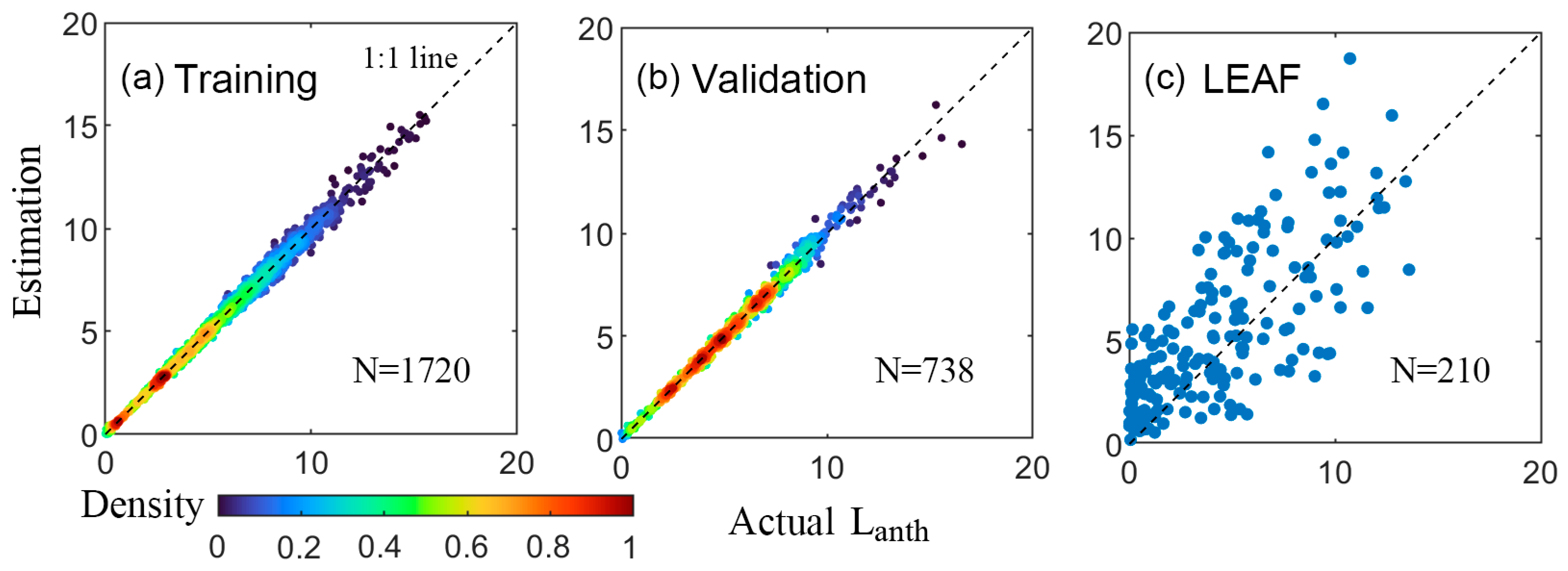
3.3. Retrieval with ANNs

Table 6 lists the retrieval results using ANNs. The models using the four VIs, reflectance, and log(1/R) at 550, 710, and 770 nm did not perform well in LEAF, yielding high RMSE values (>4 μg/cm2) and/or low R2 values (<0.4), although some models achieved excellent results in SIMU (e.g., mARI had an R2 > 0.9 and an RMSE < 0.9 μg/cm2). In comparison, when using the first six or eight PCs, the models maintained excellent performance in SIMU and significantly improved their performance in LEAF (R2 > 0.47 and RMSE < 4 μg/cm2). Notably, log(1/R) did not improve but instead decreased the model’s accuracy in LEAF (e.g., R-(PC1–PC6) vs. log-(PC1–PC6)). Models using the first six PCs performed better than those using the first eight PCs in LEAF (e.g., log-(PC1–PC6) vs. log-(PC1–PC8)). The best ANN model in LEAF was the one that used the first six PCs derived from reflectance as independent variables.
Figure 1 shows the scatterplots for actual vs. estimated Lanth values using the best ANN model (in bold in Table 6). Overall, the data points exhibit a uniform distribution along the 1:1 line, suggesting a consistent retrieval power within the content range.

3.4. Retrieval with SVM Models

Table 7 lists the retrieval results using SVM models. Similar to ANNs, SVM models using four VIs also demonstrated terrible predictive accuracy in LEAF. Except for these four VIs, the SVMs performed better than the ANN in LEAF with the same independent variables. For SVMs, log(1/R) did not necessarily improve the accuracy in LEAF compared to reflectance. For instance, log-(R550, R710, R770) performed better than (R550, R710, R770), whereas log-(PC1–PC6) showed reduced accuracy compared to R-(PC1–PC6). In addition, log-(PC1–PC6) and log-(PC1–PC8) had close R2 values (0.58 vs. 0.56), but the former had a higher RMSE (3.23 vs. 3.11 μg/cm2). Therefore, log-(PC1–PC6) was regarded as worse than log-(PC1–PC8). The best SVM model in LEAF was the one that used the first six PCs derived from reflectance as independent variables. Compared to the best ANN model (in bold in Table 6), the best SVM model achieved a lower accuracy in SIMU.
Figure 2 shows the scatterplots for actual vs. estimated Lanth values using the best SVM model (in bold in Table 7). Clearly, the model did not show consistent predictive power across the content range as it overestimated Lanth when it was <4 μg/cm2 and underestimated it when it was >6.5 μg/cm2 in both SIMU and LEAF.

3.5. Retrieval with GPR

Table 8 lists the retrieval results with GPR models. Similarly to the ANN and SVM models, the four VIs still demonstrated poor performance in LEAF. When using reflectance or log(1/R) at 550, 710, and 770 nm, the GPR models achieved excellent results in SIMU (R2 = 0.99, RMSE < 0.33 μg/cm2) but showed very low accuracy in LEAF (RMSE > 7 μg/cm2). When using six or eight PCs, GPR models maintained excellent accuracy in SIMU but had severely decreased accuracy in LEAF (all RMSEs > 20 μg/cm2). These results indicate serious overfitting in model building and thus are not included in Table 8. Significant improvements in model accuracy for LEAF were achieved only when using the first three PCs, yielding R2 values > 0.58 and RMSEs < 3 μg/cm2. Note that the first three PCs still explain 96.40%–98.63% of the total variance in the spectral data (Table 5). The best GPR model was established using the first three PCs derived from log(1/R) as independent variables.
Figure 3 shows the scatterplots for actual vs. estimated Lanth values using the best GPR model (in bold in Table 8). In comparison with the best ANN model (Figure 1), the data points exhibit a tighter distribution along the 1:1 line in LEAF and greater dispersion in training and validation, which indicates a higher accuracy in LEAF but a lower accuracy in SIMU (see also the bold in Table 6).

3.6. Retrieval with RF

The experiments showed that the RF models yielded satisfactory results with NumTrees = 100. Therefore, NumTrees was fixed at 100. The optimal MinLeafSize was searched across a range (increment = 1). All RF models with MinLeafSize in the range achieved high accuracy, and the model with the optimal MinLeafSize was the best.
The results are displayed in Table 9. Compared to the ANN, SVM, and GPR, RF models using ARI and mARI as independent variables performed well in LEAF (R2 > 0.6 and RMSE < 3.8 μg/cm2). For RF, log(1/R) improved the retrieval accuracy in LEAF compared to reflectance (e.g., (R550, R710, R770) vs. log-(R550, R710, R770)). Similarly to the ANN, the model utilizing six PCs demonstrated better accuracy in LEAF compared to its counterpart using eight PCs (e.g., R-(PC1–PC6) vs. R-(PC1–PC8)). The best RF model in LEAF was the one that employed the first six PCs derived from reflectance as independent variables.
Figure 4 shows the scatterplots for actual vs. estimated Lanth values using the best RF model (in bold in Table 9). Apparently, in both SIMU and LEAF, the model overestimated and underestimated Lanth when it was <1.3 and >9 μg/cm2, respectively.

4. Discussion

4.1. Comparison of the Four Machine Learning Methods

All the best ANN, SVM, GPR, and RF models (in bold in Table 6, Table 7, Table 8 and Table 9) obtained R2 values > 0.57 and RMSEs < 2.97 μg/cm2 in LEAF, suggesting satisfactory results to some extent. Of the four machine learning methods, however, SVM and RF did not maintain a consistent estimation power within the Lanth range of 0–14 μg/cm2 (Figure 2c and Figure 4c). In comparison, the ANN and GPR demonstrated consistent retrieval power within this range (Figure 1c and Figure 3c). Of all the models obtained, the GPR model using the first three PCs derived from log(1/R) as independent variables (the bold in Table 8) performed the best. This result is consistent with some other studies in which GPR outperformed other machine learning methods in retrieval [52,53,54]. However, it was not always the case that GPR was superior to the other three methods. For instance, Moreno-Martinez et al. [34] found that RF was more accurate than GPR in the global mapping of leaf traits. Vafaei et al. [55] reported that SVMs performed the best in forest aboveground biomass estimation, while GPR and RF ranked second and third, respectively. Ali et al. [56] showed that the ANN was better than GPR, RF, and SVM in canopy chlorophyll content retrieval. Thus, the actual performances of these methods vary among specific situations (e.g., different targeted variables and simulated and in situ data). The selection of the best model should be determined through a comprehensive comparative analysis of their performance under specific circumstances.

4.2. Hybrid vs. State-of-the-Art Direct Empirical Retrieval

As mentioned in the Introduction, empirical models in almost all previous Lanth retrieval studies were directly built from in situ data. Therefore, it is necessary to compare the performance of such direct empirical models with the hybrid method.
In our earlier study, a GPR model was directly built from LEAF, and the best results were achieved when utilizing log(1/R) at 564 nm and 705 nm, yielding R2 = 0.93 and RMSE < 2.21 nmol/cm2 (about 0.99 μg/cm2) in training and validation, respectively [22]. Moreover, as described in Section 2.3, log(1/R) at 550, 710, and 770 nm was used to build the GPR model directly from LEAF, where 10-fold cross-validation was undertaken. Other settings during model building were the same as those in Section 2.3. The obtained R2 and RMSE values between the actual and estimated Lanth were 0.89 and 1.18 μg/cm2. This accuracy is a little worse than that in our earlier study, but better than that of the present best GPR model (the bold in Table 8). Direct empirical models in other studies [21,24,25,26] also showed higher accuracy, with R2 values of 0.80–0.96. Ravi et al. [13] applied a hybrid method to estimate crop Lanth, yielding R2 = 0.52 and RMSE = 12.92 μg/cm2. This accuracy is lower than that of our best ANN, SVM, GPR, and RF models (bolded in Table 6, Table 7, Table 8 and Table 9).
Clearly, compared to the direct empirical models, the accuracy of hybrid retrieval decreased. There are two possible reasons for this situation. In the direct scheme, empirical models were directly built from the in situ dataset, which straightforwardly explores relationships among variables. Therefore, achieving high accuracy is relatively simple. In contrast, in the hybrid scheme, the simulated data were generated using a physical model, which was constructed through a series of generalizations and the simplification of actual complicated facts. For instance, the leaf mesophyll is treated as a generalized plate composed of uniformly mixed substances (water, pigments, etc.) in PROSPECT [57,58], while the real leaf mesophyll has a fine structure, such as the palisade and spongy tissues in dicotyledons. Thus, the simulated reflectance may not completely reflect certain real conditions. As shown in Figure 5, some real leaf reflectance spectra in LEAF were out of the data bounds of SIMU within some spectral ranges (e.g., 436–630 nm). We also examined other PROSPECT-D-simulated data using different sampling strategies and configurations and increased the size of the datasets (e.g., to 100,000 records). However, this issue persisted. le Maire et al. [59] also reported that some real leaf reflectance values were out of the bounds of the simulated data within some wavelengths.
On the other hand, a simulated dataset is usually much larger than an in situ dataset (2458 vs. 210 in our paper). Some simulated reflectance may be redundant for model building, thus adversely affecting retrieval. For instance, Figure 6 displays the histograms for R770 in SIMU and LEAF. According to the two-sample Kolmogorov–Smirnov test, R770 in the two datasets was from the same Gaussian distribution. However, the maxima of R770 in SIMU and LEAF were 0.631 and 0.537, respectively. Therefore, samples with R770 > 0.537 in SIMU (N = 854) may be redundant.
All these challenges reduced the accuracy of hybrid retrieval compared to empirical models directly built from in situ data. Several measures may be useful for overcoming these problems. The first is to input more information during model building. Providing more information to the models may help them more precisely depict the complicated relationships among variables. The overall superior performance of the models using the first several PCs accounting for 96.40%–99.9% of the total variance within the data over those using (R550, R710, R770), log-(R550, R710, R770), and the four VIs with the same machine learning methods (see Table 5, Table 6, Table 7, Table 8 and Table 9) confirmed the effectiveness of this approach. Second, with respect to decreasing redundancy in the simulated dataset, active learning is a promising strategy. Active learning employs an iterative procedure to optimize the training dataset and finally generates a smaller dataset that is as informative as the original one [60]. The third method is to introduce deep learning methods to hybrid retrieval. Deep learning is more powerful for learning the complicated underlying non-linear relationships between variables and usually performs better than conventional machine learning methods [61,62]. For instance, Shi et al. [40] built a convolutional neural network model to estimate forest leaf chlorophyll and carotenoid contents, and the model outperformed the ANN, SVM, and GPR models.

4.3. Potential for Lanth Mapping at the Canopy Scale

Hybrid methods combined with ANN, RF, and GPR models have been successfully employed to map vegetation traits (e.g., chlorophylls) [10,34,35,63]. Timely and accurate estimation and mapping of vegetation traits is the principal approach to monitoring vegetation dynamics. However, so far, Lanth mapping in a large region has not been reported. Ravi et al. [13] mapped crop Lanth at two study sites in a small area based on the obtained hybrid models. Nevertheless, the results reported by Ravi et al. [13] and those of the present study confirm the potential of the hybrid retrieval and mapping of vegetation Lanth. In the coming years, with the proliferation of cheap and sophisticated drones [64], the hyperspectral data of vegetation will be easily accessible. Hybrid models will also be easy to construct (e.g., in the form of our best GPR model) to estimate and map vegetation Lanth.

5. Conclusions

In this study, four typical machine learning algorithms—ANN, SVM, GPR, and RF—were investigated to estimate Lanth using a hybrid method. The results showed that all the best ANN, SVM, GPR, and RF models obtained satisfactory results, yielding R2 values > 0.57 and RMSEs < 2.97 μg/cm2 in LEAF. Overall, the models using the first several PCs accounting for 96.40%–99.9% of the variance in the data as independent variables outperformed those using VIs, (R550, R710, R770), and log-(R550, R710, R770). Among all models built, the GPR model established using the first three PCs derived from log(1/R) was the best, yielding R2 = 0.76 and RMSE = 2.24 μg/cm2 in LEAF. However, the hybrid scheme had reduced accuracy compared to retrieval using empirical models directly built from LEAF due to the uncertainty between the simulated and in situ datasets. Nevertheless, our results further verify the feasibility and power of hybrid retrieval for Lanth and illustrate the potential of hybrid methods in regional Lanth mapping. Using easily accessible drone-based hyperspectral data, hybrid models can be readily built to estimate and map vegetation Lanth.

Author Contributions

Conceptualization, Y.L. and Y.C.; methodology, Y.L.; validation, Y.L. and Q.Y.; formal analysis, Q.Y. and Y.C.; writing—original draft preparation, Y.L.; writing—review and editing, Y.L., Q.Y. and Y.C.; supervision, Y.C. All authors have read and agreed to the published version of the manuscript.

Funding

This research received no external funding.

Data Availability Statement

The data presented in this article are available on request from the authors.

Acknowledgments

We thank Anatoly Gitelson, Mark Merzlyak and all other people who made a contribution in building the in situ dataset. We appreciate Alexei Solovchenko’s opening of the leaf datasets to the public, which made this study possible. The files are available at https://www.researchgate.net/publication/319213426_Foliar_reflectance_and_biochemistry_5_data_sets (accessed on 18 March 2019).

Conflicts of Interest

The authors declare no conflicts of interest.

References

  1. Chalker-Scott, L. Environmental significance of anthocyanins in plant stress responses. Photochem. Photobiol. 1999, 70, 1–9. [Google Scholar] [CrossRef]
  2. Landi, M.; Tattini, M.; Gould, K.S. Multiple functional roles of anthocyanins in plant-environment interactions. Environ. Exp. Bot. 2015, 119, 4–17. [Google Scholar] [CrossRef]
  3. Gould, K.S. Nature’s Swiss army knife: The diverse protective roles of anthocyanins in leaves. J. Biomed. Biotechnol. 2004, 2004, 314–320. [Google Scholar] [CrossRef]
  4. Naing, A.H.; Kim, C.K. Abiotic stress-induced anthocyanins in plants: Their role in tolerance to abiotic stresses. Physiol. Plant. 2021, 172, 1711–1723. [Google Scholar] [CrossRef] [PubMed]
  5. Francis, F.J. Food Colorants—Anthocyanins. Crit. Rev. Food Sci. Nutr. 1989, 28, 273–314. [Google Scholar] [CrossRef] [PubMed]
  6. Lee, D.W.; Gould, K.S. Why leaves turn red—Pigments called anthocyanins probably protect leaves from light damage by direct shielding and by scavenging free radicals. Am. Sci. 2002, 90, 524–531. [Google Scholar] [CrossRef]
  7. Luo, L.; Chang, Q.; Gao, Y.; Jiang, D.; Li, F. Combining Different Transformations of Ground Hyperspectral Data with Unmanned Aerial Vehicle (UAV) Images for Anthocyanin Estimation in Tree Peony Leaves. Remote Sens. 2022, 14, 2271. [Google Scholar] [CrossRef]
  8. Verrelst, J.; Camps-Valls, G.; Munoz-Mari, J.; Pablo Rivera, J.; Veroustraete, F.; Clevers, J.G.P.W.; Moreno, J. Optical remote sensing and the retrieval of terrestrial vegetation bio-geophysical properties—A review. ISPRS J. Photogramm. Remote Sens. 2015, 108, 273–290. [Google Scholar] [CrossRef]
  9. Brown, L.A.; Ogutu, B.O.; Dash, J. Estimating Forest Leaf Area Index and Canopy Chlorophyll Content with Sentinel-2: An Evaluation of Two Hybrid Retrieval Algorithms. Remote Sens. 2019, 11, 1752. [Google Scholar] [CrossRef]
  10. Estevez, J.; Salinero-Delgado, M.; Berger, K.; Pipia, L.; Rivera-Caicedo, J.P.; Wocher, M.; Reyes-Munoz, P.; Tagliabue, G.; Boschetti, M.; Verrelst, J. Gaussian processes retrieval of crop traits in Google Earth Engine based on Sentinel-2 top-of-atmosphere data. Remote Sens. Environ. 2022, 273, 112958. [Google Scholar] [CrossRef]
  11. Zhang, Y.; Hui, J.; Qin, Q.; Sun, Y.; Zhang, T.; Sun, H.; Li, M. Transfer-learning-based approach for leaf chlorophyll content estimation of winter wheat from hyperspectral data. Remote Sens. Environ. 2021, 267, 112724. [Google Scholar] [CrossRef]
  12. Guo, A.; Huang, W.; Qian, B.; Ye, H.; Jiao, Q.; Cheng, X.; Ruan, C. A hybrid model coupling PROSAIL and continuous wavelet transform based on multi-angle hyperspectral data improves maize chlorophyll retrieval. Int. J. Appl. Earth Obs. Geoinf. 2024, 132, 104076. [Google Scholar] [CrossRef]
  13. Ravi, J.; Nigam, R.; Bhattacharya, B.K.; Desai, D.; Patel, P. Retrieval of crop biophysical-biochemical variables from airborne AVIRIS-NG data using hybrid inversion of PROSAIL-D. Adv. Space Res. 2024, 73, 1269–1289. [Google Scholar] [CrossRef]
  14. Féret, J.B.; Gitelson, A.A.; Noble, S.D.; Jacquemoud, S. PROSPECT-D: Towards modeling leaf optical properties through a complete lifecycle. Remote Sens. Environ. 2017, 193, 204–215. [Google Scholar] [CrossRef]
  15. Verhoef, W. Light-Scattering by Leaf Layers with Application to Canopy Reflectance Modeling—The Sail Model. Remote Sens. Environ. 1984, 16, 125–141. [Google Scholar] [CrossRef]
  16. Gamon, J.A.; Surfus, J.S. Assessing leaf pigment content and activity with a reflectometer. New Phytol. 1999, 143, 105–117. [Google Scholar] [CrossRef]
  17. Sims, D.A.; Gamon, J.A. Relationships between leaf pigment content and spectral reflectance across a wide range of species, leaf structures and developmental stages. Remote Sens. Environ. 2002, 81, 337–354. [Google Scholar] [CrossRef]
  18. Gitelson, A.A.; Merzlyak, M.N.; Chivkunova, O.B. Optical properties and nondestructive estimation of anthocyanin content in plant leaves. Photochem. Photobiol. 2001, 74, 38–45. [Google Scholar] [CrossRef]
  19. Gitelson, A.A.; Keydan, G.P.; Merzlyak, M.N. Three-band model for noninvasive estimation of chlorophyll, carotenoids, and anthocyanin contents in higher plant leaves. Geophys. Res. Lett. 2006, 33, 567. [Google Scholar] [CrossRef]
  20. Vina, A.; Gitelson, A.A. Sensitivity to Foliar Anthocyanin Content of Vegetation Indices Using Green Reflectance. IEEE Geosci. Remote Sens. Lett. 2011, 8, 464–468. [Google Scholar] [CrossRef]
  21. Gu, X.; Cai, W.; Fan, Y.; Ma, Y.; Zhao, X.; Zhang, C. Estimating foliar anthocyanin content of purple corn via hyperspectral model. Food Sci. Nutr. 2018, 6, 572–578. [Google Scholar] [CrossRef]
  22. Li, Y.; Huang, J. Leaf Anthocyanin Content Retrieval with Partial Least Squares and Gaussian Process Regression from Spectral Reflectance Data. Sensors 2021, 21, 3078. [Google Scholar] [CrossRef] [PubMed]
  23. Cherif, E.; Feilhauer, H.; Berger, K.; Dao, P.D.; Ewald, M.; Hank, T.B.; He, Y.; Kovach, K.R.; Lu, B.; Townsend, P.A.; et al. From spectra to plant functional traits: Transferable multi-trait models from heterogeneous and sparse data. Remote Sens. Environ. 2023, 292, 113580. [Google Scholar] [CrossRef]
  24. Jiang, S.; Chang, Q.; Wang, X.; Zheng, Z.; Zhang, Y.; Wang, Q. Estimation of Anthocyanins in Whole-Fertility Maize Leaves Based on Ground-Based Hyperspectral Measurements. Remote Sens. 2023, 15, 2571. [Google Scholar] [CrossRef]
  25. Zhang, Z.; Jiang, D.; Chang, Q.; Zheng, Z.; Fu, X.; Li, K.; Mo, H. Estimation of Anthocyanins in Leaves of Trees with Apple Mosaic Disease Based on Hyperspectral Data. Remote Sens. 2023, 15, 1732. [Google Scholar] [CrossRef]
  26. Miao, H.; Chen, X.; Guo, Y.; Wang, Q.; Zhang, R.; Chang, Q. Estimation of Anthocyanins in Winter Wheat Based on Band Screening Method and Genetic Algorithm Optimization Models. Remote Sens. 2024, 16, 2324. [Google Scholar] [CrossRef]
  27. van den Berg, A.K.; Perkins, T.D. Nondestructive estimation of anthocyanin content in autumn sugar maple leaves. HortScience 2005, 40, 685–686. [Google Scholar] [CrossRef]
  28. Steele, M.R.; Gitelson, A.A.; Rundquist, D.C.; Merzlyak, M.N. Nondestructive Estimation of Anthocyanin Content in Grapevine Leaves. Am. J. Enol. Vitic. 2009, 60, 87–92. [Google Scholar] [CrossRef]
  29. Gitelson, A.; Solovchenko, A. Non-invasive quantification of foliar pigments: Possibilities and limitations of reflectance- and absorbance-based approaches. J. Photochem. Photobiol. B-Biol. 2018, 178, 537–544. [Google Scholar] [CrossRef]
  30. Verrelst, J.; Munoz, J.; Alonso, L.; Delegido, J.; Pablo Rivera, J.; Camps-Valls, G.; Moreno, J. Machine learning regression algorithms for biophysical parameter retrieval: Opportunities for Sentinel-2 and -3. Remote Sens. Environ. 2012, 118, 127–139. [Google Scholar] [CrossRef]
  31. Liakos, K.G.; Busato, P.; Moshou, D.; Pearson, S.; Bochtis, D. Machine Learning in Agriculture: A Review. Sensors 2018, 18, 2674. [Google Scholar] [CrossRef] [PubMed]
  32. Verrelst, J.; Malenovsky, Z.; Van der Tol, C.; Camps-Valls, G.; Gastellu-Etchegorry, J.-P.; Lewis, P.; North, P.; Moreno, J. Quantifying Vegetation Biophysical Variables from Imaging Spectroscopy Data: A Review on Retrieval Methods. Surv. Geophys. 2019, 40, 589–629. [Google Scholar] [CrossRef]
  33. Guo, Y.; Xiao, Y.; Hao, F.; Zhang, X.; Chen, J.; de Beurs, K.; He, Y.; Fu, Y.H. Comparison of different machine learning algorithms for predicting maize grain yield using UAV-based hyperspectral images. Int. J. Appl. Earth Obs. Geoinf. 2023, 124, 103528. [Google Scholar] [CrossRef]
  34. Moreno-Martinez, A.; Camps-Valls, G.; Kattge, J.; Robinson, N.; Reichstein, M.; van Bodegom, P.; Kramer, K.; Cornelissen, J.H.C.; Reich, P.; Bahn, M.; et al. A methodology to derive global maps of leaf traits using remote sensing and climate data. Remote Sens. Environ. 2018, 218, 69–88. [Google Scholar] [CrossRef]
  35. Xu, M.; Liu, R.; Chen, J.M.; Shang, R.; Liu, Y.; Qi, L.; Croft, H.; Ju, W.; Zhang, Y.; He, Y.; et al. Retrieving global leaf chlorophyll content from MERIS data using a neural network method. ISPRS J. Photogramm. Remote Sens. 2022, 192, 66–82. [Google Scholar] [CrossRef]
  36. Gitelson, A.A.; Chivkunova, O.B.; Merzlyak, M.N. Nondestructive estimation of anthocyanins and chlorophylls in anthocyanic leaves. Am. J. Bot. 2009, 96, 1861–1868. [Google Scholar] [CrossRef]
  37. Merzlyak, M.N.; Chivkunova, O.B.; Solovchenko, A.E.; Naqvi, K.R. Light absorption by anthocyanins in juvenile, stressed, and senescing leaves. J. Exp. Bot. 2008, 59, 3903–3911. [Google Scholar] [CrossRef]
  38. Quan, X.; He, B.; Li, X. A Bayesian Network-Based Method to Alleviate the Ill-Posed Inverse Problem: A Case Study on Leaf Area Index and Canopy Water Content Retrieval. IEEE Trans. Geosci. Remote 2015, 53, 6507–6517. [Google Scholar] [CrossRef]
  39. Feret, J.-B.; Francois, C.; Gitelson, A.; Asner, G.P.; Barry, K.M.; Panigada, C.; Richardson, A.D.; Jacquemoud, S. Optimizing spectral indices and chemometric analysis of leaf chemical properties using radiative transfer modeling. Remote Sens. Environ. 2011, 115, 2742–2750. [Google Scholar] [CrossRef]
  40. Shi, S.; Xu, L.; Gong, W.; Chen, B.; Chen, B.; Qu, F.; Tang, X.; Sun, J.; Yang, J. A convolution neural network for forest leaf chlorophyll and carotenoid estimation using hyperspectral reflectance. Int. J. Appl. Earth Obs. Geoinf. 2022, 108, 102719. [Google Scholar] [CrossRef]
  41. Li, Y.; Liang, S. Evaluation of Reflectance and Canopy Scattering Coefficient Based Vegetation Indices to Reduce the Impacts of Canopy Structure and Soil in Estimating Leaf and Canopy Chlorophyll Contents. IEEE Trans. Geosci. Remote 2023, 61, 3266500. [Google Scholar] [CrossRef]
  42. Beale, R.; Jackson, T. Neural Computing: An Introduction; IOP Publishing Ltd.: Bristol, UK, 1990. [Google Scholar]
  43. Ojha, V.K.; Abraham, A.; Snasel, V. Metaheuristic design of feedforward neural networks: A review of two decades of research. Eng. Appl. Artif. Intell. 2017, 60, 97–116. [Google Scholar] [CrossRef]
  44. Vapnik, V.N. The Nature of Statistical Learning Theory; Springer: New York, NY, USA, 1995. [Google Scholar]
  45. Smola, A.J.; Schölkopf, B. A tutorial on support vector regression. Stat. Comput. 2004, 14, 199–222. [Google Scholar] [CrossRef]
  46. Sun, D.; Li, Y.; Wang, Q. A Unified Model for Remotely Estimating Chlorophyll a in Lake Taihu, China, Based on SVM and <i>In Situ</i> Hyperspectral Data. IEEE Trans. Geosci. Remote 2009, 47, 2957–2965. [Google Scholar] [CrossRef]
  47. Mehdizadeh, S.; Behmanesh, J.; Khalili, K. Using MARS, SVM, GEP and empirical equations for estimation of monthly mean reference evapotranspiration. Comput. Electron. Agric. 2017, 139, 103–114. [Google Scholar] [CrossRef]
  48. Rasmussen, C.E.; Williams, C.K.I. Gaussian Processes for Machine Learning; The MIT Press: Cambridge, MA, USA, 2006. [Google Scholar]
  49. Camps-Valls, G.; Verrelst, J.; Munoz-Mari, J.; Laparra, V.; Mateo-Jimenez, F.; Gomez-Dan, J. A Survey on Gaussian Processes for Earth-Observation Data Analysis A comprehensive investigation. IEEE Geosci. Remote Sens. Mag. 2016, 4, 58–78. [Google Scholar] [CrossRef]
  50. Breiman, L. Random forests. Mach. Learn. 2001, 45, 5–32. [Google Scholar] [CrossRef]
  51. Dormann, C.F.; Elith, J.; Bacher, S.; Buchmann, C.; Carl, G.; Carre, G.; Garcia Marquez, J.R.; Gruber, B.; Lafourcade, B.; Leitao, P.J.; et al. Collinearity: A review of methods to deal with it and a simulation study evaluating their performance. Ecography 2013, 36, 27–46. [Google Scholar] [CrossRef]
  52. de Sa, N.C.; Baratchi, M.; Hauser, L.T.; van Bodegom, P. Exploring the Impact of Noise on Hybrid Inversion of PROSAIL RTM on Sentinel-2 Data. Remote Sens. 2021, 13, 648. [Google Scholar] [CrossRef]
  53. Verrelst, J.; Pablo Rivera, J.; Veroustraete, F.; Munoz-Mari, J.; Clevers, J.G.P.W.; Camps-Valls, G.; Moreno, J. Experimental Sentinel-2 LAI estimation using parametric, non-parametric and physical retrieval methods—A comparison. ISPRS J. Photogramm. Remote Sens. 2015, 108, 260–272. [Google Scholar] [CrossRef]
  54. Ashourloo, D.; Aghighi, H.; Matkan, A.A.; Mobasheri, M.R.; Rad, A.M. An Investigation Into Machine Learning Regression Techniques for the Leaf Rust Disease Detection Using Hyperspectral Measurement. IEEE J. Sel. Top. Appl. Earth Obs. Remote Sens. 2016, 9, 4344–4351. [Google Scholar] [CrossRef]
  55. Vafaei, S.; Soosani, J.; Adeli, K.; Fadaei, H.; Naghavi, H.; Pham, T.D.; Bui, D.T. Improving Accuracy Estimation of Forest Aboveground Biomass Based on Incorporation of ALOS-2 PALSAR-2 and Sentinel-2A Imagery and Machine Learning: A Case Study of the Hyrcanian Forest Area (Iran). Remote Sens. 2018, 10, 172. [Google Scholar] [CrossRef]
  56. Ali, A.M.; Darvishzadeh, R.; Skidmore, A.; Gara, T.W.; Heurich, M. Machine learning methods’ performance in radiative transfer model inversion to retrieve plant traits from Sentinel-2 data of a mixed mountain forest. Int. J. Digit. Earth 2021, 14, 106–120. [Google Scholar] [CrossRef]
  57. Jacquemoud, S.; Baret, F. Prospect—A Model of Leaf Optical-Properties Spectra. Remote Sens. Environ. 1990, 34, 75–91. [Google Scholar] [CrossRef]
  58. Allen, W.A.; Gausman, H.W.; Richardson, A.J.; Thomas, J.R. Interaction of Isotropic Light with a Compact Plant Leaf. J. Opt. Soc. Am. 1969, 59, 1376–1379. [Google Scholar] [CrossRef]
  59. le Maire, G.; François, C.; Dufrêne, E. Towards universal broad leaf chlorophyll indices using PROSPECT simulated database and hyperspectral reflectance measurements. Remote Sens. Environ. 2004, 89, 1–28. [Google Scholar] [CrossRef]
  60. Berger, K.; Rivera Caicedo, J.P.; Martino, L.; Wocher, M.; Hank, T.; Verrelst, J. A Survey of Active Learning for Quantifying Vegetation Traits from Terrestrial Earth Observation Data. Remote Sens. 2021, 13, 287. [Google Scholar] [CrossRef] [PubMed]
  61. LeCun, Y.; Bengio, Y.; Hinton, G. Deep learning. Nature 2015, 521, 436–444. [Google Scholar] [CrossRef]
  62. Yuan, Q.; Shen, H.; Li, T.; Li, Z.; Li, S.; Jiang, Y.; Xu, H.; Tan, W.; Yang, Q.; Wang, J.; et al. Deep learning in environmental remote sensing: Achievements and challenges. Remote Sens. Environ. 2020, 241, 111716. [Google Scholar] [CrossRef]
  63. Xiao, Z.; Liang, S.; Wang, J.; Chen, P.; Yin, X.; Zhang, L.; Song, J. Use of General Regression Neural Networks for Generating the GLASS Leaf Area Index Product From Time-Series MODIS Surface Reflectance. IEEE Trans. Geosci. Remote 2014, 52, 209–223. [Google Scholar] [CrossRef]
  64. Maes, W.H.; Steppe, K. Perspectives for Remote Sensing with Unmanned Aerial Vehicles in Precision Agriculture. Trends Plant Sci. 2019, 24, 152–164. [Google Scholar] [CrossRef] [PubMed]
Figure 1. Actual vs. estimated Lanth values (μg/cm2) in (a) training, (b) validation, and (c) LEAF datasets using the best ANN model (in bold in Table 6).
Forests 16 00804 g001
Figure 2. Actual vs. estimated Lanth values (μg/cm2) in (a) training, (b) validation, and (c) LEAF datasets using the best SVM model (in bold in Table 7).
Forests 16 00804 g002
Figure 3. Actual vs. estimated Lanth values (μg/cm2) in (a) training, (b) validation, and (c) LEAF datasets using the best GPR model (in bold in Table 8).
Forests 16 00804 g003
Figure 4. Actual vs. estimated Lanth values (μg/cm2) in (a) training, (b) validation, and (c) LEAF datasets using the best RF model (in bold in Table 9).
Forests 16 00804 g004
Figure 5. All reflectance in LEAF (light gray) and the formed lower and upper bounds (red lines). The black lines are the lower and upper bounds of the reflectance in SIMU.
Forests 16 00804 g005
Figure 6. Histograms (20 bins) for R770 in SIMU and LEAF. The red lines are Gaussian lines fitted to R770, with the fitted mean (μ) and standard deviation (σ) shown in the top left. The two-sample Kolmogorov–Smirnov (KS) test result demonstrates that R770 values in SIMU and LEAF were from the same Gaussian distribution (P = 1).
Forests 16 00804 g006
Table 1. Input parameters and their configurations for the PROSPECT-D model. STD stands for standard deviation.
ParameterSymbolUnitRangeMean, STD
Leaf structureNunitless1–32, 1
Chlorophyll contentCabμg/cm20.02–5511.9, 11.5
Carotenoid contentCcarμg/cm20.04–102.8, 1.7
Anthocyanin contentLanthμg/cm20–174.1, 3.8
Brown pigment contentCbrownarbitraryFixed at 0
Equivalent water thicknessCwcm0.0002–0.0380.016, 0.007
Dry matter contentCmg/cm20.0001–0.0290.0086, 0.0035
Table 2. Correlation coefficient (r) matrix for 6 parameters (excluding Cbrown) in Table 1.
NCabCcarLanthCwCm
N1.00−0.15−0.02−0.030.300.13
Cab−0.151.000.65−0.120.190.50
Ccar−0.020.651.000.250.250.40
Lanth−0.03−0.120.251.000.200.30
Cw0.300.190.250.201.000.70
Cm0.130.500.400.300.701.00
Table 3. Some VIs for Lanth estimation. Rx means reflectance at the wavelength x nm.
NameFormulaReference
Red/GreenR680/R550[22]
ARI1/R550 − 1/R700[18]
mARI(1/R550 − 1/R700) × R770[19]
mACIR770/R550[28]
Table 4. Descriptive statistics of pigment contents (μg/cm2) in LEAF. The contents of chlorophyll-a, chlorophyll-b, and carotenoids were not measured in hazel leaves, so these leaves were excluded from the statistics of chlorophylls and carotenoids.
PigmentRangeMeanStandard
Deviation
Pearson’s Correlation Coefficient (r)
ChlorophyllsCarotenoidsAnthocyanins
Chlorophylls0.06–48.3011.72 11.371.000.64 1−0.10 2
Carotenoids0.08–6.752.32 1.57 0.64 11.000.23 1
Anthocyanins0–13.583.99 3.62 −0.10 20.23 11.00
1 p < 0.01, 2 p < 0.05.
Table 5. The accumulative percentage (%) of the total variance explained by the first 10 PCs in the spectral data.
Spectral DataPC1PC2PC3PC4PC5PC6PC7PC8PC9PC10
LEAF76.97 92.24 96.40 98.07 98.99 99.72 99.85 99.91 99.95 99.97
log-LEAF75.65 95.09 97.67 98.72 99.48 99.76 99.85 99.92 99.95 99.97
SIMU77.12 91.59 98.35 99.10 99.73 99.95 99.98 99.99 100.00 100.00
log-SIMU82.23 96.51 98.63 99.54 99.86 99.97 99.99 100.00 100.00 100.00
Table 6. Retrieval results using ANNs. Neuron(s) represents the number of neurons in the hidden layer. (R550, R710, R770) represent reflectance at 550, 710, and 770 nm, respectively, while log-(R550, R710, R770) indicates their log(1/R) values. R-(PC1–PC6) represents PC1, PC2, …, and PC6 derived from reflectance, while log-(PC1–PC6) represents PC1, PC2, …, and PC6 derived from log(1/R), with similar meanings for for R-(PC1–PC8) and log-(PC1–PC8). The bold indicates the best of all ANN models for LEAF.
Independent VariableNeuron(s)R2RMSE (μg/cm2)
TrainingValidationIn situTrainingValidationIn Situ
Red/Green10.420.420.392.362.283.60
ARI30.830.840.721.281.214.32
mARI40.930.930.750.810.775.32
mACI100.770.750.421.481.525.03
(R550, R710, R770)10.930.910.790.810.885.12
log-(R550, R710, R770)130.990.990.480.260.335.51
R-(PC1–PC6)60.990.990.580.250.282.96
R-(PC1–PC8)40.990.990.540.290.363.87
log-(PC1–PC6)30.990.990.520.270.313.46
log-(PC1–PC8)30.990.990.480.230.293.58
Table 7. Retrieval results using SVMs. The bold indicates the best of all SVM models for LEAF.
Independent VariableR2RMSE (μg/cm2)
TrainingValidationIn SituTrainingValidationIn Situ
Red/Green0.440.430.362.322.283.61
ARI0.840.820.541.261.274.14
mARI0.930.940.370.820.764.35
mACI0.770.750.201.491.515.27
(R550, R710, R770)0.890.880.701.121.103.34
log-(R550, R710, R770)0.610.590.702.702.633.22
R-(PC1–PC6)0.810.790.621.831.792.58
R-(PC1–PC8)0.800.790.531.561.532.60
log-(PC1–PC6)0.990.990.580.270.333.23
log-(PC1–PC8)0.990.980.560.330.373.11
Table 8. Retrieval results using GPR. R-(PC1–PC3) represents PC1, PC2, and PC3 derived from reflectance, while log-(PC1–PC3) represents PC1, PC2, and PC3 derived from log(1/R). The bold indicates the best of the GPR models for LEAF.
Independent VariableR2RMSE (μg/cm2)
TrainingValidationIn SituTrainingValidationIn Situ
Red/Green0.440.430.322.312.263.80
ARI0.830.840.681.291.194.60
mARI0.930.940.450.810.774.92
mACI0.770.750.521.501.525.65
R550, R710, R7700.990.990.860.270.327.49
log-(R550, R710, R770)0.990.990.790.270.327.76
R-(PC1–PC3)0.970.960.590.530.602.69
log-(PC1–PC3)0.830.820.761.281.272.24
Table 9. Retrieval results using RFs. The bold indicates the best of all RF models for LEAF.
Independent VariableMinLeafSize (Search Range)R2RMSE (μg/cm2)
TrainingValidationIn SituTrainingValidationIn Situ
Red/Green93 (50–100)0.450.430.382.302.273.65
ARI298 (250–300)0.780.790.611.441.373.32
mARI148 (90–150)0.910.910.640.930.933.75
mACI147 (90–150)0.760.730.451.531.584.42
(R550, R710, R770)60 (50–100)0.880.850.591.391.423.23
log-(R550, R710, R770)95 (50–100)0.830.790.581.581.593.21
R-(PC1–PC6)57 (50–100)0.900.870.561.161.262.65
R-(PC1–PC8)51 (50–100)0.900.860.541.091.222.70
log-(PC1–PC6)59 (50–100)0.920.900.661.051.102.33
log-(PC1–PC8)77 (50–100)0.910.890.651.111.152.38
Disclaimer/Publisher’s Note: The statements, opinions and data contained in all publications are solely those of the individual author(s) and contributor(s) and not of MDPI and/or the editor(s). MDPI and/or the editor(s) disclaim responsibility for any injury to people or property resulting from any ideas, methods, instructions or products referred to in the content.

