Analysis of Forest Change Detection Induced by Hurricane Helene Using Remote Sensing Data

Abstract

The occurrence of hurricanes in the southern U.S. is on the rise, and assessing the damage caused to forests is essential for implementing protective measures and comprehending recovery dynamics. This work aims to create a novel data integration framework that employs LANDSAT 8, drone-based images, and geographic information system data for change detection analysis for different forest types. We propose a method for change vector analysis based on a unique spectral mixture model utilizing composite spectral indices along with univariate difference imaging to create a change detection map illustrating disturbances in the areas of McDowell County in western North Carolina impacted by Hurricane Helene. The spectral indices included near-infrared-to-red ratios, a normalized difference vegetation index, Tasseled Cap indices, and a soil-adjusted vegetation index. In addition to the satellite imagery, the ground truth data of forest damage were also collected through the field investigation and interpretation of post-Helene drone images. Accuracy assessment was conducted with geographic information system (GIS) data and maps from the National Land Cover Database. Accuracy assessment was carried out using metrics such as overall accuracy, precision, recall, F score, Jaccard similarity, and kappa statistics. The proposed composite method performed well with overall accuracy and Jaccard similarity values of 73.80% and 0.6042, respectively. The results exhibit a reasonable correlation with GIS data and can be employed to assess damage severity.

1. Introduction

Hurricanes constitute a significant natural disruption to forest ecosystems in the southeastern United States. A powerful hurricane may significantly impact the composition, structure, and succession of forests [1,2]. The increasing number of forest disturbances and their severity in the recent past necessitates prompt and precise local forest damage assessments to facilitate post-hurricane forest management after the hurricane, hazardous fuel control and mitigation, relief activities, and administrative compensation requests [3,4]. Western North Carolina has traditionally suffered considerable flooding and destruction from weakening hurricanes or their leftovers, despite being situated well inland from coastal areas that usually experience the most severe and widely reported effects. This results from heavy rainfall that can lead to the considerable swelling of rivers and water bodies, along with torrents cascading down hilly regions, resulting in destruction and damage [5]. Hurricane Helene made landfall on Florida’s Gulf Coast on 26 September 2024, as a powerful category 4 hurricane, including maximum sustained winds of 140 miles per hour. Helene arrived in North Carolina on 27 September 2024, by which time the western section of the state had already experienced significant rainfall. Helene produced far greater precipitation, resulting in three-day rainfall totals of over 8 inches in North Carolina’s mountainous region and over 12 inches in some locations. The highest local rainfall maxima in the state surpassed 30 inches for only the second occasion in reported history [6].

A precise assessment of the extent and intensity of areas affected by the hurricane, along with the identification of factors influencing the spatial distribution of the disturbance, is crucial for local and national governments to facilitate post-hurricane relief efforts, inform decision-making, and enhance risk management. Traditional methods for evaluating damage and quantifying losses rely on site visits to gather information via questionnaires, interviews, and photographs for preliminary assessment [7,8,9,10]. Nevertheless, acquiring comprehensive information necessitates significant time (days or weeks) contingent upon the accessibility and extent of the harm in the impacted region. Therefore, the development of enhanced, efficient approaches for quantifying damage losses in less time and with minimal labor is of particular significance.

Many existing studies have relied on satellite remote sensing, utilizing changes in various vegetation indices as indicators of affected forest areas, with limited attempts to assess their quantitative correlation with forest damage at the pixel level and few comparative analyses regarding their efficacy [11,12,13,14,15]. Landsat datasets were utilized for quantitative damage assessment of vegetation dynamics [11] and cyclone damage to dry forests [15]. Change detection in remote sensing entails utilizing two or more aerial or satellite images of the same geographic region to identify changes in land use and land cover characteristics during a period. Change detection processes typically encompass the preprocessing of satellite imagery, feature extraction, the application of change detection methodologies, and the evaluation of accuracy. Image preprocessing typically involves a sequence of operations, including the reduction in atmospheric effects on radiance, precise image registration, the extraction of areas of interest, and the conversion of images to indices that exhibit a robust correlation between their values and land cover attributes. The majority of change detection methodologies employ per-pixel classifiers, such as the post-classification comparison technique, and rely on pixel-based change information derived from the spectral domain of the images [16,17]. Change detection methods, like univariate image differencing (UID), are needed to spot changes by looking at the pixel-level information in images. UID is a method in which the pixel values of the spectral index or remote sensing imagery from one date are subtracted from another date [17]. The disparity in areas with no change will be minimal, whereas places of change will have substantial positive or negative values.

Spectral indices are derived from basic band arithmetic procedures, utilizing the distinct reflectance patterns of land cover and land use objects across various energy spectra [18,19,20,21]. The prior methodologies can be categorized into numerous groups according to the spectral indices derived from the separate physical principles employed in forest canopy detection: (1) detection utilizing changes in chlorophyll concentration [22,23,24], (2) detection employing variations in the presence of water content in leaves [25,26,27,28,29], and (3) detection based on spectral mixture signatures [30,31,32,33,34,35]. The authors in [30] described the application of spectral mixture analysis, which illustrated a viable method for retrieving different types of vegetation. Their methodology depended on endmember classification utilizing high-resolution images. Nevertheless, limited research has documented the quantitative evaluation of forest damage following hurricanes.

This study extends past remote sensing research by integrating spectral indices with GIS data to provide a more detailed and accurate assessment of post-hurricane forest damage across different forest types—deciduous, evergreen, and mixed. This research identifies a composite spectral mixture model tailored to specific forest classifications, enhancing damage detection precision. Furthermore, the study introduces a validated methodology for post-hurricane damage assessment, supported by independent field surveys and GIS datasets, which strengthens the reliability and applicability of the findings in real-world disaster response and forest management scenarios.

This paper aims to investigate the efficacy of widely utilized spectral indices in detecting post-hurricane damage and to integrate GIS data for evaluating damage severity in hurricane-affected areas. The explicit objectives of this study are to (1) identify a reliable composite spectral mixture model for detecting affected areas and assessing damage severity in deciduous, evergreen, and mixed forest types, (2) implement and analyze a methodology for post-hurricane assessment, and (3) validate this methodology using independent field surveys and GIS data.

2. Materials and Methods

2.1. Study Area and Datasets

The study area covers McDowell County, located within the southern Appalachian Mountains region in the western part of North Carolina, USA (Figure 1). Forests in this county cover roughly 75% of the total area, which is 445 square miles [36]. A set of two Landsat Operational Land Imager (OLI) images (path 18, row 35) was collected. The first was taken on 30 August 2024, before Hurricane Helene’s landfall, and the second on 17 October 2024, with cloud cover of less than 10%; the projection coordinate system was Universal Transverse Mercator (UTM); the geographic coordinate system was WGS84. The full-scene Landsat 8 image size is 7771 rows × 7901 columns. Because of the cloud-free conditions, we did not carry out any atmospheric correction of the image. We derived all the spectral indices from these images. It was presumed that throughout this brief timeframe, no more disruptions transpired in the study area aside from the damage caused by Hurricane Helene.

To facilitate the image processing and execute change detection techniques, three other geographically referenced datasets were collected: (1) GIS data layer from NHQRedCrossGIS [37] and 2018 TIGER/Line shapefiles from the Environmental Systems Research Institute as shown in Figure 2a, and (2) training and validation samples were collected from National Land Cover Database (NLCD) class maps 2023 (All Annual NLCD Landcover 2023 with accuracy 80.4–90.6%) [38] as shown in Figure 2b. (3) We conducted a field survey on 14 November 2024 to collect reference data samples using drone and mobile cameras. Figure 3 and Figure 4 show the location points and collected images, respectively. Images P2 and P6 in Figure 4 were captured by drone. We used the Skydio 2 drone (Skydio Inc., Redwood City, CA, USA) with a 12.3 MP 1/2.3″ CMOS sensor capable of shooting 4 K video at 60 fps and 12 MP still photos. Skydio 2 was selected due to its advanced AI-assisted flight technology, high-resolution imaging capabilities, and precise autonomous navigation, which collectively enhanced the quality, consistency, and reliability of aerial image collection. Its camera features a wide 126° field of view and advanced image stabilization, including electronic image stabilization (EIS). The field inventory images in McDowell County focused on damage in upland forest areas and river floodplains. Data processing and analysis were carried out in ArcGIS Pro version 3.3 from Environmental Systems Research Institute, Redlands, CA, USA.

2.2. Methodology

This study was conducted utilizing the workflows depicted in Figure 5 to attain its objectives. The primary steps encompass (1) data acquisition, comprising training and validation datasets, Landsat 8 imagery, and supplementary data; (2) the preprocessing of Landsat images; (3) the exclusion of non-forest areas and the delineation of various forest masks; (4) the computation of spectral indices; (5) the implementation of the UID and spectral mixture models to identify forest damage; (6) the validation of the resultant forest damage; and (7) the generation and analysis of the final outputs.

Spectral indices (SI), including NDVI, TCG, TCW, RVI, SAVI, and NDWI, were derived from the Landsat dataset using the equations specified in

Table 1. Spectral Indices.

SI	Equations in Terms of Bands of Landsat 8
NDVI [18]	(B5 − B4)/(B5 + B4)
SAVI [19]	(B5 − B4)(1 + L)/(B5 + B4 + L)
RVI [19]	B5/B4
TCW [20]	0.1509.B2 + 0.1973.B3 + 0.3279.B4 + 0.3406.B5 − 0.7112.B6 − 0.4512.B7
TCG [20]	−0.2848.B2 − 0.2435.B3 − 0.5436.B4 + 0.7243.B5 + 0.084.B6 − 0.18B7
NDWI [21]	(B5 − B6)/(B5 − B6)

. The prevalent indicators in remote sensing change detection include the normalized difference vegetation index (NDVI), the ratio of near-infrared to red images (RVI), the Tasseled Cap greenness index (TCG), the Tasseled Cap wetness index (TCW), and the soil-adjusted vegetation index (SAVI). The indices can quantify the presence and density of green vegetation, overall reflectance (e.g., distinguishing between bright and dark soils), as well as soil moisture content [18]. NDVI, ranging from −1 to +1, is arguably the most widely utilized metric for identifying variations in green biomass due to seasons, natural disturbances, and human activities. It differentiates green vegetation from other surfaces due to chlorophyll absorption in the red spectrum and reflection in the near-infrared spectrum. Consequently, higher NDVI values signify substantial leaf biomass, canopy closure, leaf area, and the quantity of photosynthetically active green biomass. NDVI is unable to distinguish between very dense and dense canopies because of the restricted penetration ability of reflected red spectra, a phenomenon known as the saturation problem. The saturation issue of NDVI may restrict its capacity to identify minor damage in densely forested areas. Higher soil-induced noise in NDVI estimates may lead to erroneous interpretations of vegetation cover [18]. RVI, the first ratio-based vegetation index, closely resembles NDVI but exhibits more sensitivity to dense forests. RVI exhibits the greatest sensitivity at higher leaf area index values [19]. Consequently, RVI may more effectively distinguish between damage levels in wind-disturbed forests compared to those affected by logging or fire. SAVI is a transformation method that reduces the impact of soil brightness on spectral values, including red and near-infrared wavelengths, such as NDVI and RVI [19]. The utilization of SAVI can significantly reduce the estimation inaccuracy of plant cover caused by soil brightness, unlike NDVI, especially when the proportion of vegetation cover is minimal [19]. TCW has been used to assess the structural complexity and age of mature forest stands and to identify changes in forests. The estimation of vegetation water content generally employs values from liquid water absorption channels in the shortwave infrared (SWIR) spectra, contrasting them with values from channels that are unaffected by liquid water in the near-infrared (NIR) spectra [20]. Numerous indices utilizing NIR and SWIR channels have been established, including the normalized difference water index (NDWI) [21]. The adjustment factor (L) in the SAVI equation was set at 0.5. Designating L as 0.5 accurately reflects the average intermediate forest density. An increment in L beyond 0.5 will amplify background effects due to soil in SAVI [19].

The forested areas, prior to Helene, were analyzed using pre-Helene images, categorizing them into 20 classes, including deciduous, evergreen, and mixed forests, aligned with the twenty classes of NLCD land cover data. The imagery was subsequently grouped into three categories (deciduous, evergreen, and mixed forests) utilizing the signature file and visual inspection. Only the categories identified as forests or those potentially qualifying as forests were carefully analyzed, assessed, and categorized through visual inspection of the NLCD data. The obtained forestland imagery was used as a stencil for change images and was utilized as a reference for identifying forest disturbances.

The UID method generates continuous change images by subtracting the post-Helene spectral index (SI) imagery from the pre-Helene SI, thereby highlighting the variations in spectral responses due to hurricane damage. The spectral index change detection map is calculated as

$$D(x,y)=I_2(x,y)-I_1(x,y)$$

(1)

where D(x, y) is the change in spectral index at pixel location (x, y), I₂(x, y) is the spectral index pixel value at (x, y) in the post-event image, and I₁(x, y) is the spectral index pixel value at (x, y) in the pre-event image.

In an optimal scenario, if forest cover was modified by Helene, UID will produce a higher magnitude indicating affected forests, while zero or close-to-zero numbers denote undisturbed forests in the continuous change images. To detect the magnitude of changes in the proposed spectral mixture analysis, we employ the change vector algorithms described in Equations (2)–(9). We calculated the magnitudes of changes using a quadratic-square-root function of the spectral indices before and after Helene.

$$M1=\sqrt{{\left(NDV{I}_{post}-NDV{I}_{pre}\right)}^2+{\left(SAV{I}_{post}-SAV{I}_{pre}\right)}^2}$$

(2)

$$M2=\sqrt{{\left(TC{G}_{post}-TC{G}_{pre}\right)}^2+{\left(TC{W}_{post}-TC{W}_{pre}\right)}^2}$$

(3)

$$M3=\sqrt{{\left(NDV{I}_{post}-NDV{I}_{pre}\right)}^2+{\left(TC{W}_{post}-TC{W}_{pre}\right)}^2+{\left(SAV{I}_{post}-SAV{I}_{pre}\right)}^2+{\left(RV{I}_{post}-RV{I}_{pre}\right)}^2}$$

(4)

$$M4=\sqrt{{\left(NDV{I}_{post}-NDV{I}_{pre}\right)}^2+{\left(TC{W}_{post}-TC{W}_{pre}\right)}^2+{\left(RV{I}_{post}-RV{I}_{pre}\right)}^2}$$

(5)

$$M5=\sqrt{{\left(TC{W}_{post}-TC{W}_{pre}\right)}^2+{\left(RV{I}_{post}-RV{I}_{pre}\right)}^2}$$

(6)

$$M6=\sqrt{{\left(NDV{I}_{post}-NDV{I}_{pre}\right)}^2+{\left(NDW{I}_{post}-NDW{I}_{pre}\right)}^2}$$

(7)

$$M7=\sqrt{{\left(NDW{I}_{post}-NDW{I}_{pre}\right)}^2+{\left(SAV{I}_{post}-SAV{I}_{pre}\right)}^2}$$

(8)

$$M8=\sqrt{{\left(NDV{I}_{post}-NDV{I}_{pre}\right)}^2+{\left(NDW{I}_{post}-NDW{I}_{pre}\right)}^2+{\left(SAV{I}_{post}-SAV{I}_{pre}\right)}^2}$$

(9)

The design of these index combinations was to evaluate whether incorporating more pairs of indices enhances change detection accuracy and to ascertain if a modified vector containing several indices is more effective in identifying disturbances than the UID method. A range of approaches has been devised for detecting land cover changes [39,40,41,42,43,44]. These methods identify land cover changes using thresholds determined by specific methods or through manual trial-and-error techniques, which are intricate to execute and may undermine both reliability and accuracy [45]. This study utilized Natural Breaks (Jenks, OK, USA) in ArcGIS Pro to classify the changed images to account for non-uniform distributions. The reference map, comprising three categories (deciduous forest, evergreen forest, and mixed forest), was produced from the specified classes (classes #41, #42, and #43) in the NLCD-2023 database. A change detection map was generated from the two classification maps and compared with those built using ∆SI tiles and the outputs of spectral mixture models (M1–M8). A separate cross-validation and accuracy evaluation were performed by examining changed and unchanged pixels from the change detection maps in terms of precision, recall, overall accuracy (OA), F-ratio, kappa statistics (KSs), and Jaccard similarity (JS).

The percentage of the area affected was computed to assess the extent of impact across different mixture models. The impact of each spectral index on the change detection map was examined by statistical distribution analysis. The mean of the ∆SI, shift amplitude (SA), and statistical dispersion measured by the interquartile range (IQR) were used to evaluate the precision of the change detection map. The change detection maps were analyzed with the GIS data layer from NHQRedCrossGIS across multiple severity levels. The ground truth data were used for validation.

The predominant metrics employed to assess a binary classification (change vs. no-change) technique are precision and recall. The precision is computed as the ratio of predicted changed pixels classified as changed, while recall is calculated as the ratio of all labeled changed pixels that are correctly predicted as defined in Equations (10) and (11) [46]. F-score, overall accuracy (OA), kappa statistics (KSs), and Jaccard similarity (JS) were utilized for quantitative evaluation as defined in Equations (12)–(14) [46].

• TP (true positive) represents the number of changed pixels that have been properly classified as changed pixels.
• FP (false positive) represents the number of non-changed pixels being misclassified as changed.
• FN (false negative) represents the number of changed pixels being misclassified as non-changed.
• TN (true negative) represents the number of non-changed pixels that have been properly classified as non-changed pixels.

The performance metrics are as follows, as defined in [46]:

Precision = TP/(TP + FP)

(10)

Recall = TP/(TP + FN)

(11)

F-score = 2TP/(2TP + FP + FN)

(12)

Overall accuracy = (TP + TN)/(TP + TN + FN + FP)

(13)

Jaccard Similarity = TP/(TP + FP + FN)

(14)

3. Results

3.1. Change Detection Analysis

Table 2. Performance using UID spectral indices (all forests).

SI	Precision	Recall	F1	OA	KS	JS
NDVI	0.6578	0.6869	0.7019	0.6792	0.4012	0.5324
SAVI	0.6792	0.6432	0.6945	0.6618	0.4122	0.5104
RVI	0.6624	0.6295	0.6821	0.6382	0.3082	0.4964
TCG	0.5670	0.5286	0.6042	0.5421	0.2461	0.4264
TCW	0.6072	0.6271	0.6176	0.6192	0.3712	0.4492
NDWI	0.6892	0.6932	0.7007	0.6918	0.4132	0.6182

SI: spectral index; OA: overall accuracy; KS: kappa statistics; JS: Jaccard similarity.

details the performance of UID-based change detection using different spectral indices. The overall accuracy and KS values of the classification ranged from 54.21% to 69.18% and from 0.2461 to 0.4132, respectively (Table 2). The overall accuracies and KS values of the NDVI and SAVI vegetation indexes were comparable. The accuracies attained by RVI and TCW were similar, ranging narrowly from 61.92% to 63.82%. TCG has the lowest precision (0.5670) and recall (0.5286), indicating that it struggles the most in terms of correctly predicting positives and finding all true positives. This results in the lowest F1 score (0.6042) and OA (0.5421). TCW performs slightly better than TCG, with a precision of 0.6072 and a recall of 0.6271, leading to a higher F1 score (0.6176) and OA (0.6192). However, it still lags other indices in terms of performance. Despite a strong correlation between NDVI and RVI, NDVI appeared to be better than RVI at identifying affected areas. Among all the individual indices considered in this study, change detection with NDWI resulted in higher accuracy (69.18%), signifying that NDWI effectively recorded forest changes caused by Hurricane Helene.

Figure 6 shows the change maps produced by different mixture models. The overall accuracy and kappa statistics of the classification ranged from 58.80% to 73.80% and from 0.13 to 0.48, respectively (

Table 3. Performance using spectral mixture models (all forests).

SM Model	Precision	Recall	F1	OA	KS	JS
M1	0.7752	0.7299	0.7519	0.7360	0.47	0.6024
M2	0.6961	0.7774	0.7345	0.6920	0.38	0.5804
M3	0.5872	0.8358	0.6898	0.5880	0.13	0.5264
M4	0.5872	0.8358	0.6898	0.5880	0.13	0.5264
M5	0.7553	0.6533	0.7006	0.6940	0.39	0.5392
M6	0.7519	0.7299	0.7407	0.7200	0.43	0.5882
M7	0.7752	0.7299	0.7519	0.7360	0.48	0.6024
M8	0.7782	0.7299	0.7533	0.7380	0.48	0.6042

SM: spectral mixture; OA: overall accuracy; KS: kappa statistics; JS: Jaccard similarity.

). The M8 model, utilizing a composite index signature of NDVI, NDWI, and SAVI, had the best overall accuracy and KS, making it the most promising method. Models M7 and M8 showed almost similar results in terms of overall accuracy and kappa statistics. Models M3 and M4 were found to be ineffective compared to the other models as both these mixture models are composed of the TCW and RVI indices, which are found to be weaker in detecting the changes. The M8 model captured the forest changes with the highest overall accuracy at 73.80% and a precision of 0.7782.

Figure 7 illustrates the change maps generated by various models for deciduous forest lands. The overall accuracies and KS values of the classification ranged from 71.60% to 81.80% and from 0.25 to 0.59, respectively (

Table 4. Performance using spectral mixture models for deciduous forest.

SM Model	Precision	Recall	F1	OA	KS	JS
M1	0.8932	0.8190	0.8545	0.8120	0.51	0.7459
M2	0.8189	0.8724	0.8448	0.7840	0.49	0.7313
M3	0.7327	0.9110	0.8122	0.7160	0.25	0.6837
M4	0.7327	0.9110	0.8122	0.7160	0.25	0.6837
M5	0.8800	0.7834	0.8289	0.7820	0.53	0.7078
M6	0.8750	0.8309	0.8524	0.8060	0.57	0.7427
M7	0.8907	0.8220	0.8549	0.8120	0.58	0.7466
M8	0.8968	0.8249	0.8594	0.8180	0.59	0.7534

SM: spectral mixture; OA: overall accuracy; KS: kappa statistics; JS: Jaccard similarity.

). Model M8 had the highest value in most metrics. M7 and M1 were also high-performing models, with M1 having a slightly lower JS (0.7459) compared to M8. M3 and M4 showed similar performance with relatively lower precision (0.7327) and F1 score (0.8122), but they excelled in recall (0.9110), indicating they are very good at identifying true positives, though they have a higher number of false positives. M5 shows strong precision (0.8800), but its recall is slightly lower (0.7834), which suggests a better compromise between recall and precision compared to the M3 and M4 models. M8 has the highest JS (0.7534), indicating that it has the best overlap between predicted and actual sets.

Figure 8 illustrates the change maps generated by various models for evergreen forest lands. The performance across all 8 models (M1 to M8) is very similar, with only slight variations. The precision, recall, F1 score, OA, and JS values are extremely high across all models, as the sample size is not too large. Most models have precision and recall values around 0.9798 to 0.9980, and F1 scores are consistently above 0.9858 (

Table 5. Performance using spectral mixture models for evergreen forests.

SM Model	Precision	Recall	F1	OA	KS	JS
M1	0.9798	0.9959	0.9878	0.9760	0.24	0.9759
M2	0.9779	0.9980	0.9878	0.9760	0.13	0.9760
M3	0.9780	1.0000	0.9889	0.9780	0.15	0.9780
M4	0.9780	1.0000	0.9889	0.9780	0.15	0.9780
M5	0.9759	0.9959	0.9858	0.9720	0.14	0.9720
M6	0.9798	0.9959	0.9878	0.9760	0.24	0.9759
M7	0.9798	0.9959	0.9878	0.9760	0.24	0.9759
M8	0.9798	0.9959	0.9878	0.9760	0.24	0.9759

SM: spectral mixture; OA: overall accuracy; KS: kappa statistics; JS: Jaccard similarity.

). The JS values are very high across all models, indicating that the predicted sets closely align with the actual sets. The values are all around 0.9759 to 0.9780, which shows that the predictions are highly similar to the true data.

Figure 9 illustrates the change maps generated by various models for mixed forest lands. M1, M7, and M8 show the highest precision (0.9512 for M1 and M7, 0.9513 for M8) and F1 score (0.9544 for M1 and M7, 0.9556 for M8), with M1 and M7 also having the highest OA (0.9180) (

Table 6. Performance using spectral mixture models for mixed forest.

SM Model	Precision	Recall	F1	OA	KS	JS
M1	0.9512	0.9576	0.9544	0.9180	0.53	0.9128
M2	0.9296	0.9732	0.9509	0.9100	0.41	0.9064
M3	0.9084	0.9955	0.9499	0.9060	0.2	0.9047
M4	0.9084	0.9955	0.9499	0.9060	0.2	0.9047
M5	0.9084	0.9955	0.9499	0.9060	0.51	0.9047
M6	0.9495	0.9643	0.9568	0.9220	0.55	0.9172
M7	0.9512	0.9576	0.9544	0.9180	0.54	0.9128
M8	0.9513	0.9598	0.9556	0.9200	0.55	0.9149

SM: spectral mixture; OA: overall accuracy; KS: kappa statistics; JS: Jaccard similarity.

). These models have consistently strong performance across all metrics. M3, M4, and M5 have lower precision (0.9084) compared to M1, M7, and M8, but they have perfect recall (0.9955). This means they are highly sensitive to detecting true positives, though they might have more false positives. M3 and M4 have lower KS values (0.2), indicating that these models have less discrimination ability between the two classes, despite their high recall.

3.2. Post-Helene Forest Damage Assessment

Figure 10 shows the map of forest damage severity generated by different mixture models (M1–M8). It depicts the distribution of forest damage on a scale from 0 to 1 at the pixel level. The pixels depicted in white indicate no damage, whereas the pixels in light yellow, light gray, light magenta, and dark magenta signify varying degrees of damage, from light to most severe. This study employed Natural Breaks (Jenks) in ArcGIS Pro to categorize the changed outputs (M1–M8) in order to account for non-uniform distributions. We used five categories of severity for detailed analysis. While this map offers damage data at a nominal resolution of 900 m² (30 m × 30 m) per pixel, forest managers may want broader information to effectively oversee post-hurricane hazard abatement efforts.

Figure 11 shows the contribution of different models in detecting damage levels. M8, M7, and M1 are the models that detect the most severe impacts, with M8 showing the highest detection in both the destroyed (4.81) and major impact (17.30) categories. These models seem to be the most sensitive to detecting significant damage in forest areas. Models M3 and M4 detect the most unaffected areas, suggesting they tend to be more focused on identifying regions that have not been impacted, while their detection of severe impacts is lower. M2 is more focused on minor impact areas and detects fewer severe impacts. It was observed that the model M8 performs better compared to other models. We conducted further analysis using the M8 model in terms of deciduous, evergreen, and mixed forest types.

Figure 12 shows the map of forest damage severity for deciduous, evergreen, and mixed forest types using the M8 model. For evergreen forests, most impacts fall into the minor to moderate categories. Figure 13 presents the probability map corresponding to the detected forest changes. In this map, areas highlighted in red represent high probability values (closer to 1), indicating a strong likelihood of change, while areas in blue correspond to low probability values (closer to 0), suggesting little to no change. The spatial distribution of these probabilities aligns well with the change detection results shown in Figure 12d, thereby reinforcing the reliability of the classification outputs and offering additional insight into the confidence of detected changes. This probability layer can support more informed decision-making by allowing users to prioritize areas for field validation, further analysis, or targeted management actions based on confidence levels.

Figure 14 shows the damage severity comparison between different types of forest. Deciduous forest appears to be more impacted, especially in the minor impact and moderate impact categories, suggesting it may be more vulnerable to damage than the other types. Evergreen forests show minimal destruction and major impact, which could be due to the resilience of evergreen trees or their ability to withstand harsher conditions. This capability may be attributed to the structural characteristics and nutrition cycles of evergreen trees. Mixed forests show moderate values across the impact categories, but like the evergreen forest, they have a large unaffected portion, indicating some level of resilience across both deciduous and evergreen forest types. Both evergreen forest and mixed forest have a large portion that remains unaffected by any impact, with the evergreen forest being the most resilient (96.95%). Deciduous forest also has a significant unaffected portion (43.60%), but this is still less than the other two forest types. The evergreen forest shows a significantly high value for the unaffected category (96.95%), indicating that most of this forest type remains untouched. However, the destroyed and major impact categories have very low values, indicating that this forest type has experienced very little destruction or major damage. The moderate impact and minor impact categories have slightly higher values, but they are still much lower than the unaffected category. For the mixed forest, the highest values appear in the unaffected category (82.79%), like the evergreen forest. The minor impact and moderate impact categories follow with values of 7.49% and 6.80%, respectively. The destroyed and major impact categories have relatively small values, showing that mixed forests experience less severe damage than other forest types.

3.3. Affected Area Analysis

Further analysis is carried out in terms of area estimates for the damage severity maps. Figure 15a shows a total forest–affected area estimate comparison. Models M7 and M8 appear to detect more severe impacts compared to other models, with the largest areas of destroyed and major impact detected. M6 is particularly sensitive to moderate impact areas, detecting a large area (128.23 square miles), which suggests it excels at identifying areas with moderate damage. M2 seems to identify minor impact areas the most, detecting the largest area (206.74 square miles). The finding suggests that M2 may be more focused on identifying less severe damage and potentially has a lower sensitivity for more extreme impacts. M3 and M4 detect the largest areas of unaffected land, suggesting that these models may be more conservative or restrictive in identifying affected areas.

Figure 15b illustrates the affected area estimates for different types of forests. In the deciduous forest, the largest affected areas are in the minor impact category, followed by moderate impact, major impact, and finally the destroyed category, which has the smallest affected area. The evergreen forest has minimally affected areas in all categories, with the largest being in the minor impact category. The destroyed category has a minimal area (0.05 square miles), indicating that the evergreen forest is the least impacted in terms of destruction compared to the other impact categories. In the mixed forest, like the deciduous forest, the largest area affected is in the minor impact category, followed by moderate impact, major impact, and destroyed, with the smallest affected area. Deciduous and mixed forests have larger affected areas across all impact categories, particularly in the minor and moderate impact categories, indicating a wider range of disturbances. The low values in all categories indicate that the evergreen forest is likely less impacted overall compared to deciduous and mixed forests, possibly due to its specific ecological characteristics, such as resilience to disturbances.

4. Discussion

To visually compare the sensitivity of different indices in the proposed mixture models for detecting forest damage, pre- and post-Helene histograms of NDVI, NDWI, SAVI, and TCW are presented in Figure 16. As models M1, M7, and M8 are found to be better-performing models in terms of precision, F1 score, OA, and JS, we investigate their constituent spectral indices NDVI, NDWI, and SAVI for statistical comparison. Consistent with the work in [47], we observed from the results of the multiple spectral signatures that using more than one spectral index can be quite advantageous for forest disturbance detection. The authors in [47] examined the utility of multiple spectral indices and corresponding correlations to detect improved forest disturbances in an ensemble setting. These results further align with the findings in [48]. Spectral indices based on three conceptually independent categories corresponding to soil, vegetation, and moisture characteristics improved the accuracy of forest change detection [48]. To enhance the study, the histograms employ lines rather than traditional bar charts to depict the distribution of ∆SIs. The amplitude of the change was directly correlated with the sensitivity of these indices to hurricane impacts. The authors in [49] utilized NDVI, TCG, and TCB to evaluate change detection using remote sensing images for land cover applications for improved performance. The larger shift in ∆NDVI (0.11) as compared to ∆SAVI (0.09), ∆TCG (0.05), and ∆TCW (0.08) contributed to improved accuracy (

Table 7. Statistics of ∆SI.

∆SI	Mean	SD	SA	IQR
∆NDVI	0.0820	0.0459	0.11	0.279
∆SAVI	0.1241	0.0681	0.09	0.280
∆TCG	0.3124	0.0734	0.05	0.021
∆TCW	0.0312	0.0834	0.08	0.051
∆RVI	0.3953	0.2042	0.09	0.192
∆NDWI	0.0791	0.0495	0.14	0.319

SD: standard deviation, SA: shift in amplitude, IQR: interquartile range.

). This result is in agreement with the work presented in [49]. The NDVI–albedo combination was found to be better than the TCG–TCB-based combinations [49]. This result also aligns with the outcome presented in [50] to assess the desertification risk using change vector analysis.

The shift amplitude of ∆NDWI (0.14) exceeded that of ∆TCW, ∆NDVI, and ∆SAVI, as illustrated in Figure 16 and Table 7. The large shift amplitude of ∆NDWI means the number of pixels with decreased NDWI after the hurricane increased significantly, as found in models M7 and M8. The shift amplitude of ∆NDVI (0.11) was a bit greater than that of ∆SAVI and ∆RVI (0.09), although it remained of lesser importance in comparison to the shift amplitude of ∆NDWI. This aligns with the findings in [51], which exploited NDWI signatures to detect changed pixels with improved detection rates. TCG distributions before and after Helene showed no discernible changes, suggesting that the index is not affected by the hurricane’s effects on the canopy’s greenness and the forest structures. This distinct exhibition of spectral characteristics also facilitated similar change detection, as reported in [52].

The interquartile range (IQR) as a measure of statistical dispersion reflects the ability of an indicator to differentiate between levels of forest damage severity. An indicator with significant dispersion can more effectively distinguish levels of damage severity compared to other indications. The proportion of damaged forest pixels detectable by an indicator reflects the indicator’s overall capability in identifying impacted areas. The statistical dispersion of ∆SIs (Table 7) demonstrated the index’s sensitivity to varying levels of damage severity. The substantial interquartile range of ∆NDWI (0.319) indicated that the higher ∆NDWI values in the left tail exceeded those of ∆NDVI and ∆SAVI.

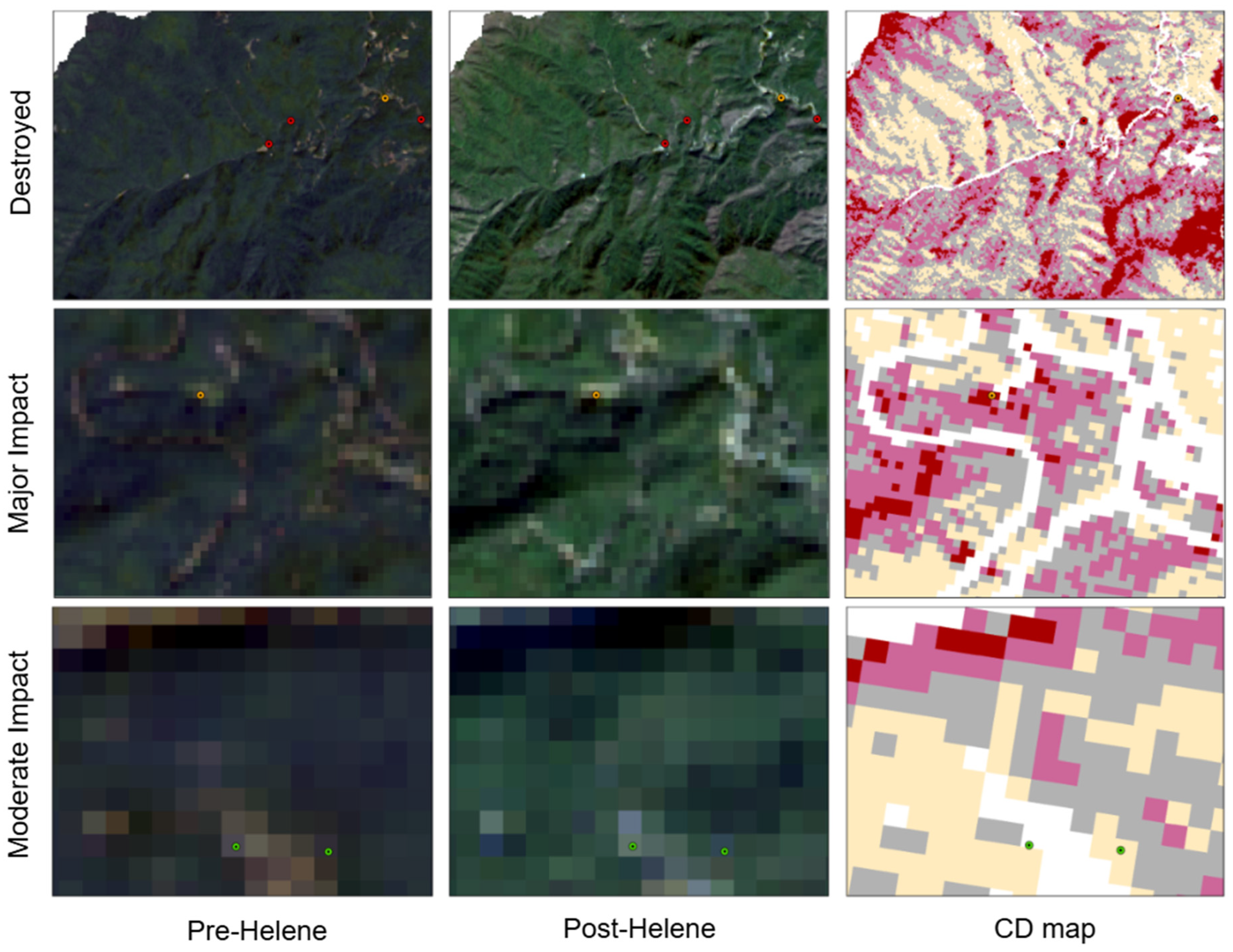
To clearly show how well our proposed method works, we present samples with different levels of damage and validation points from GIS data in Figure 17. The pixels showing destroyed areas, as well as those with major and minor damage, are found and examined in comparison to the sample tiles before and after Helene, along with the changes in the change detection map and the GIS data points. The change map results align with the GIS data points as indicated by the red, orange, and green points in Figure 17. The impacted areas indicated by the proposed mixture model of composite indices turned out to be more consistent with different damage severity.

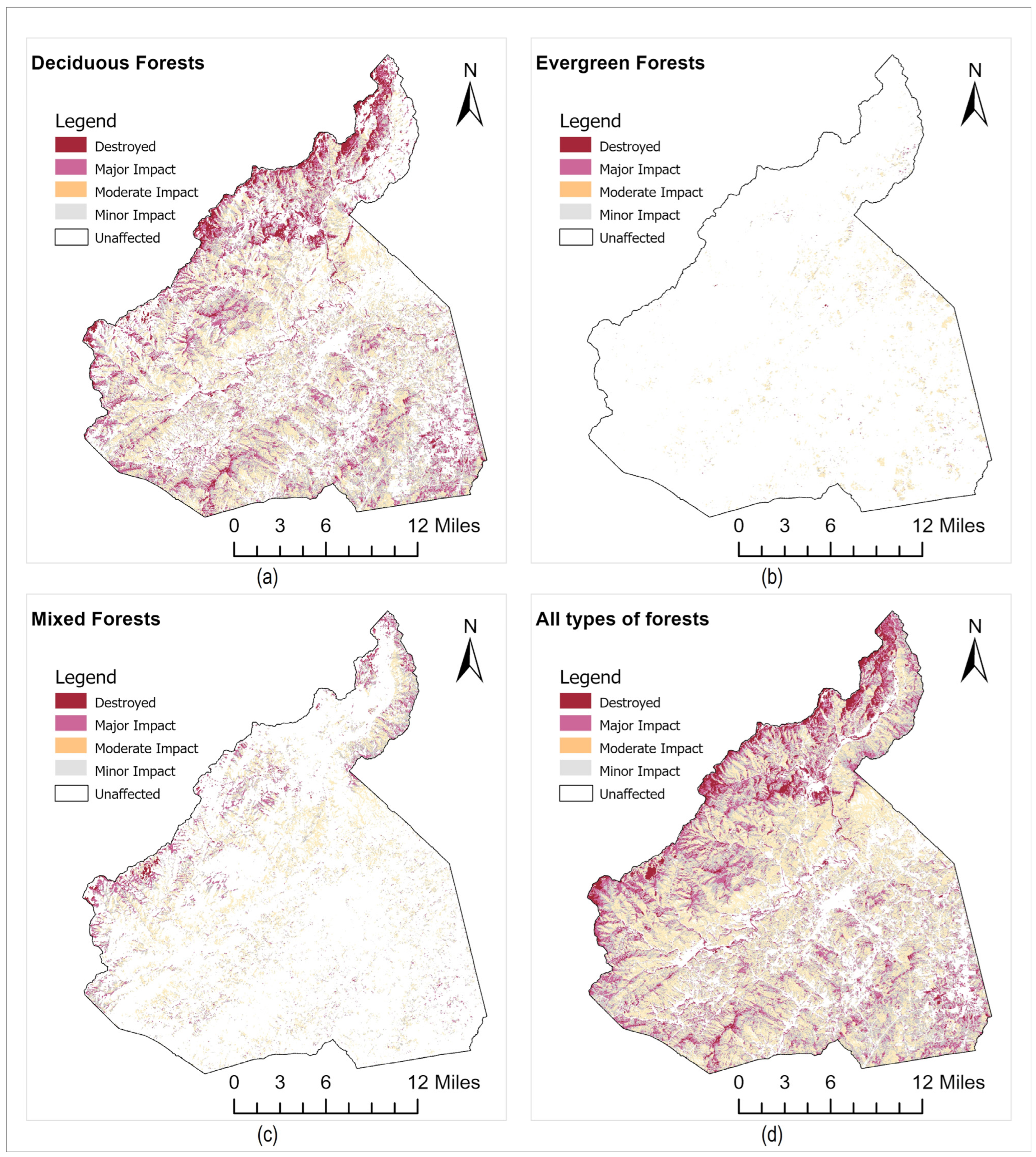
The forest damage leads to the loss of critical ecological structures with varying impacts across forest types. In predominantly deciduous stands—dominated by oaks, maples, and hickories—hurricanes often cause widespread crown damage and stem breakage. Mature canopy trees, particularly oaks, are highly susceptible due to their height and extensive crown area [53]. However, mid-story and shade-tolerant species like Acer rubrum often survive and proliferate in the increased light environment, altering post-disturbance composition [54]. Over the long term, the loss of dominant canopy species may reduce carbon storage and biodiversity, though natural regeneration processes support eventual recovery. Evergreen forests, especially those containing eastern white pine and hemlock, are vulnerable to windthrow and snap during severe hurricanes. Recovery in these forests is often slower due to limited resprouting ability and lower species diversity [55]. Mixed forests, common at mid-elevations, tend to exhibit more complex and variable responses. Their diversity can enhance resilience, but recovery depends on the balance of shade-tolerant and pioneer species [56]. Following hurricane disturbance, studies in the Southern Appalachians have documented increased dominance of red maple and birch species, sometimes at the expense of oaks and other late-successional trees [57]. Understanding these dynamics is crucial for forest management and conservation strategies. Monitoring recovery trajectories through high-resolution time series analysis can assist in distinguishing areas of potential recovery from those requiring active intervention.

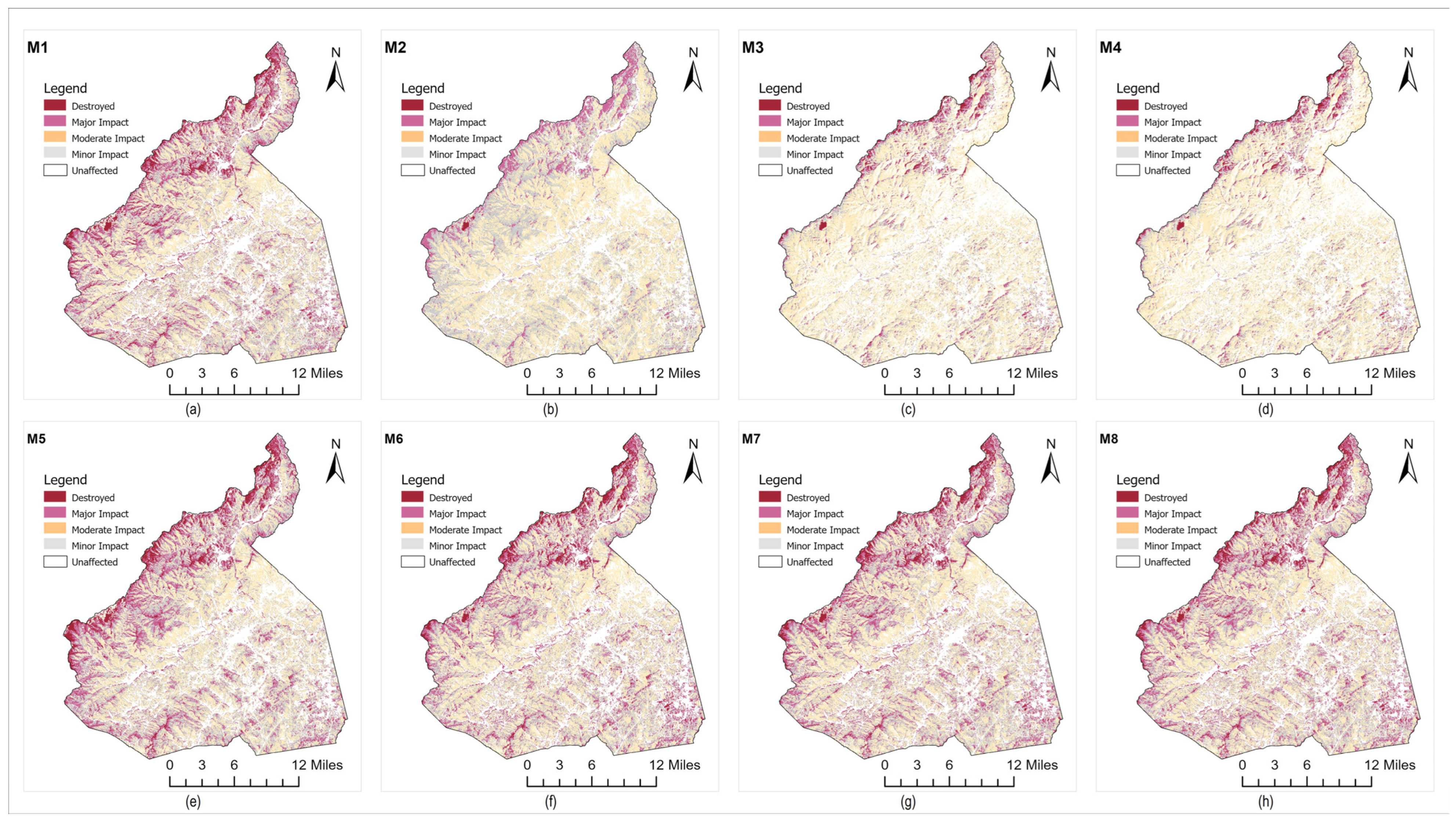
Among the models tested, M8, M7, and M1 demonstrate the highest sensitivity in detecting severe forest damage, with M8 consistently outperforming the others across both the “destroyed” and “major impact” categories. A key novel contribution of this study is the use of composite index combinations, particularly in M8, which leverages synergistic information from spectral indices. This composite approach enhances the model’s capacity to distinguish between varying levels of forest damage, enabling more nuanced assessments compared to other models. The integration of indices such as NDVI, NDWI, and SAVI contributes to the superior performance of M8, highlighting the value of combining spectral features in post-hurricane forest damage detection. The findings, while derived from a specific case study, have potential for generalization to other hurricane-impacted forest ecosystems, especially those with similar vegetation types and canopy structures. However, local calibration may be necessary to account for variations in forest composition, topography, and hurricane intensity. To ensure timely application during future hurricane events, this workflow can be updated and reproduced rapidly using satellite images and pre-configured processing scripts. A set of updated composite indices can be generated within days of image availability, allowing rapid post-disaster assessments. The success of composite models suggests that this methodology could be adapted and applied to other regions prone to hurricane disturbances. Factors such as index sensitivity to subtle vegetation changes, cloud cover interference, and limitations due to satellite pixel resolution can introduce variability in detection accuracy. For example, cloud-obscured scenes may lead to incomplete or misclassified damage zones, while coarse spatial resolution may obscure small-scale disturbances. Future work could incorporate time series analysis using high-resolution images and uncertainty quantification methods, such as confidence intervals or ensemble modeling, to better represent these limitations and improve the robustness of damage assessments.

5. Conclusions

This study provided an extensive assessment of the forest regions affected by Hurricane Helene in McDowell County, western North Carolina, utilizing spectral mixture models and a change vector technique with Landsat 8 data. Index-wise impact severity was analyzed and validated with independent GIS data and ground samples for deciduous, evergreen, and mixed forest types. The statistical analysis and damage severity comparison and change detection maps using a model based on NDVI, NDWI, and SAVI was found to be an optimal model for detecting changes due to the hurricane out of eight models utilizing other indices, including TCG, TCW, and RVI. Most of the affected forest areas experienced light and moderate damage severity. The accuracy checks showed that the suggested mixture model method was better than using individual spectral indices, achieving an overall accuracy of 73.80%. As our severity thresholds were computed based on the statistical characteristics of the data, it is probable that the thresholds in other areas might differ—such enhancements could broaden this methodology to other post-disturbance evaluations. The time series analysis of high-resolution images with ensemble modeling could be a future direction to refine findings. These findings may be utilized for forest management strategies, such as prioritizing salvage logging or reforestation efforts in the most affected areas. Additionally, emergency planning and disaster response teams can use these models to rapidly identify zones of high damage, aiding in logistical planning and resource allocation.

References

1. Hogan, J.A.; Zimmerman, J.K.; Thompson, J.; Uriarte, M.; Swenson, N.G.; Condit, R.; Hubbell, S.; Johnson, D.J.; Sun, I.F.; Chang-Yang, C.-H.; et al. The Frequency of Cyclonic Wind Storms Shapes Tropical Forest Dynamism and Functional Trait Dispersion. Forests 2018, 9, 404. [Google Scholar] [CrossRef]
2. Henderson, J.D.; Abt, R.C.; Abt, K.L.; Baker, J.; Sheffield, R. Impacts of Hurricanes on Forest Markets and Economic Welfare: The Case of Hurricane Michael. For. Policy Econ. 2022, 140, 102735. [Google Scholar] [CrossRef]
3. Rice, J.R.; Balaguru, K.; Staid, A.; Xu, W.; Judi, D. Projected Increases in Tropical Cyclone-Induced U.S. Electric Power Outage Risk. Environ. Res. Lett. 2025, 20, 034030. [Google Scholar] [CrossRef]
4. Park, G. A Comprehensive Analysis of Hurricane Damage across the U.S. Gulf and Atlantic Coasts Using Geospatial Big Data. ISPRS Int. J. Geo-Inf. 2021, 10, 781, Erratum in ISPRS Int. J. Geo-Inf. 2022, 11, 73. [Google Scholar] [CrossRef]
5. Saleem, M.; Arfan, M.; Ansari, K.; Hassan, D. Analyzing the Impact of Ungauged Hill Torrents on the Riverine Floods of the River Indus: A Case Study of Koh E Suleiman Mountains in the DG Khan and Rajanpur Districts of Pakistan. Resources 2023, 12, 26. [Google Scholar] [CrossRef]
6. Cooper, R. Hurricane Helene Recovery; Office of State Budget and Management: Raleigh, NC, USA, 2024. Available online: https://www.osbm.nc.gov/hurricane-helene-dna/open (accessed on 15 December 2024).
7. Lozano, J.-M.; Tien, I. Data Collection Tools for Post-Disaster Damage Assessment of Building and Lifeline Infrastructure Systems. Int. J. Disaster Risk Reduct. 2023, 94, 103819. [Google Scholar] [CrossRef]
8. Vafadari, A.; Philip, G.; Jennings, R. Damage Assessment And Monitoring of Cultural Heritage Places in a Disaster and Post-Disaster Event—A Case Study of Syria. Int. Arch. Photogramm. Remote Sens. Spat. Inf. Sci. 2017, 42, 695–701. [Google Scholar] [CrossRef]
9. Bird, D.K. The Use of Questionnaires for Acquiring Information on Public Perception of Natural Hazards and Risk Mitigation—A Review of Current Knowledge and Practice. Nat. Hazards Earth Syst. Sci. 2009, 9, 1307–1325. [Google Scholar] [CrossRef]
10. Platt, S.; Brown, D.; Hughes, M. Measuring Resilience and Recovery. Int. J. Disaster Risk Reduct. 2016, 19, 447–460. [Google Scholar] [CrossRef]
11. Salim, M.Z.; Kafy, A.A.; Altuwaijri, H.A.; Miah, M.T.; Jodder, P.K.; Rahaman, Z.A. Quantitative Assessment of Hurricane Ian’s Damage on Urban Vegetation Dynamics Utilizing Landsat 9 in Fort Myers, Florida. Phys. Chem. Earth Parts A/B/C 2024, 136, 103750. [Google Scholar] [CrossRef]
12. Wang, W.; Qu, J.J.; Hao, X.; Liu, Y.; Stanturf, J.A. Post-Hurricane Forest Damage Assessment Using Satellite Remote Sensing. Agric. For. Meteorol. 2010, 150, 122–132. [Google Scholar] [CrossRef]
13. Karaer, A.; Ulak, M.B.; Abichou, T.; Arghandeh, R.; Ozguven, E.E. Post-Hurricane Vegetative Debris Assessment Using Spectral Indices Derived from Satellite Imagery. Transp. Res. Rec. J. Transp. Res. Board 2021, 2675, 504–523. [Google Scholar] [CrossRef]
14. Ill, E.W.R.; Chappell, D.K.; Baldwin, D.G. AVHRR Lmagery Used to Identify Hurricane Damage in a Forested Wetland of Louisiana. Photogramm. Eng. Remote Sens. 1997, 63, 293–297. [Google Scholar]
15. Cortés-Ramos, J.; Farfán, L.M.; Herrera-Cervantes, H. Assessment of Tropical Cyclone Damage on Dry Forests Using Multispectral Remote Sensing: The Case of Baja California Sur, Mexico. J. Arid. Environ. 2020, 178, 104171. [Google Scholar] [CrossRef]
16. Goswami, A.; Sharma, D.; Mathuku, H.; Gangadharan, S.M.P.; Yadav, C.S.; Sahu, S.K.; Pradhan, M.K.; Singh, J.; Imran, H. Change Detection in Remote Sensing Image Data Comparing Algebraic and Machine Learning Methods. Electronics 2022, 11, 431. [Google Scholar] [CrossRef]
17. Liu, S.; Marinelli, D.; Bruzzone, L.; Bovolo, F. A Review of Change Detection in Multitemporal Hyperspectral Images: Current Techniques, Applications, and Challenges. IEEE Geosci. Remote Sens. Mag. 2019, 7, 140–158. [Google Scholar] [CrossRef]
18. Rouse, J.W.; Haas, R.H.; Schell, J.A.; Deering, D.W. Monitoring Vegetation Systems in the Great Plains with ERTS. In Proceedings of the Third Earth Resources Technology Satellite-1 Symposium, Volume 1: Technical Presentations, Section A, 1 January 1974. [Google Scholar]
19. Coppin, P.; Jonckheere, I.; Nackaerts, K.; Muys, B.; Lambin, E. Review ArticleDigital Change Detection Methods in Ecosystem Monitoring: A Review. Int. J. Remote Sens. 2004, 25, 1565–1596. [Google Scholar] [CrossRef]
20. CRIST, E. Vegetation and Soils Information Contained in Transformed Thematic Mapper Data. In Proceedings of the IGARSS’ 86 Symposium, Zurich, Switzerland, 8–11 September 1986; p. 1465. [Google Scholar]
21. Gao, B. NDWI—A Normalized Difference Water Index for Remote Sensing of Vegetation Liquid Water from Space. Remote Sens. Environ. 1996, 58, 257–266. [Google Scholar] [CrossRef]
22. Ramsey, R.D.; Brothers, S.M.; Cobo, M.; Wurtsbaugh, W.A. Spatiotemporal Patterns of Chlorophyll-a Concentration in a Hypersaline Lake Using High Temporal Resolution Remotely Sensed Imagery. Remote Sens. 2025, 17, 430. [Google Scholar] [CrossRef]
23. Thenkabail, P.S.; Lyon, J.G.; Huete, A. (Eds.) Hyperspectral Remote Sensing of Vegetation; CRC Press: Boca Raton, FL, USA, 2012; ISBN 9781439845370. [Google Scholar]
24. Zarco-Tejada, P.J.; Berni, J.A.J.; Suárez, L.; Sepulcre-Cantó, G.; Morales, F.; Miller, J.R. Imaging Chlorophyll Fluorescence with an Airborne Narrow-Band Multispectral Camera for Vegetation Stress Detection. Remote Sens. Environ. 2009, 113, 1262–1275. [Google Scholar] [CrossRef]
25. Hoshino, B.; Tian, Y.; Shima, K.; Riga, S.; Enkhtuvshin, Z.; McCarthy, C.; Purevtseren, M. Remotely Sensed Method for Detection of Spatial Distribution Pattern of Dryland Plants in Water Limited Ecosystem. In Proceedings of the IGARSS 2020-2020 IEEE International Geoscience and Remote Sensing Symposium, Waikoloa, HI, USA, 26 September 2020; pp. 2799–2802. [Google Scholar]
26. Konings, A.G.; Saatchi, S.S.; Frankenberg, C.; Keller, M.; Leshyk, V.; Anderegg, W.R.L.; Humphrey, V.; Matheny, A.M.; Trugman, A.; Sack, L.; et al. Detecting Forest Response to Droughts with Global Observations of Vegetation Water Content. Glob. Change Biol. 2021, 27, 6005–6024. [Google Scholar] [CrossRef] [PubMed]
27. Villacrés, J.; Arevalo-Ramirez, T.; Fuentes, A.; Reszka, P.; Auat Cheein, F. Foliar Moisture Content from the Spectral Signature for Wildfire Risk Assessments in Valparaíso-Chile. Sensors 2019, 19, 5475. [Google Scholar] [CrossRef] [PubMed]
28. Wu, Y.; Hou, Z.; Liu, Y.; Liu, W. Leaf Moisture Content Detection Method Based on UHF RFID and Hyperdimensional Computing. Forests 2024, 15, 1798. [Google Scholar] [CrossRef]
29. Tanase, M.A.; Villard, L.; Pitar, D.; Apostol, B.; Petrila, M.; Chivulescu, S.; Leca, S.; Borlaf-Mena, I.; Pascu, I.-S.; Dobre, A.-C.; et al. Synthetic Aperture Radar Sensitivity to Forest Changes: A Simulations-Based Study for the Romanian Forests. Sci. Total Environ. 2019, 689, 1104–1114. [Google Scholar] [CrossRef]
30. Chambers, J.Q.; Asner, G.P.; Morton, D.C.; Anderson, L.O.; Saatchi, S.S.; Espírito-Santo, F.D.B.; Palace, M.; Souza, C. Regional Ecosystem Structure and Function: Ecological Insights from Remote Sensing of Tropical Forests. Trends Ecol. Evol. 2007, 22, 414–423. [Google Scholar] [CrossRef]
31. Roberts, D.A.; Numata, I.; Holmes, K.; Batista, G.; Krug, T.; Monteiro, A.; Powell, B.; Chadwick, O.A. Large Area Mapping of Land-cover Change in Rondônia Using Multitemporal Spectral Mixture Analysis and Decision Tree Classifiers. J. Geophys. Res. 2002, 107, LBA 40-1–LBA 40-18. [Google Scholar] [CrossRef]
32. De Luca, G.; Modica, G.; Silva, J.M.N.; Praticò, S.; Pereira, J.M.C. Assessing Tree Crown Fire Damage Integrating Linear Spectral Mixture Analysis and Supervised Machine Learning on Sentinel-2 Imagery. Int. J. Digit. Earth 2023, 16, 3162–3198. [Google Scholar] [CrossRef]
33. Chehata, N.; Orny, C.; Boukir, S.; Guyon, D.; Wigneron, J.P. Object-Based Change Detection in Wind Storm-Damaged Forest Using High-Resolution Multispectral Images. Int. J. Remote Sens. 2014, 35, 4758–4777. [Google Scholar] [CrossRef]
34. Vohland, M.; Stoffels, J.; Hau, C.; Schüler, G. Remote Sensing Techniques for Forest Parameter Assessment: Multispectral Classification and Linear Spectral Mixture Analysis. Silva Fenn. 2007, 41, 441. [Google Scholar] [CrossRef]
35. Souza, C.M.; Roberts, D.A.; Cochrane, M.A. Combining Spectral and Spatial Information to Map Canopy Damage from Selective Logging and Forest Fires. Remote Sens. Environ. 2005, 98, 329–343. [Google Scholar] [CrossRef]
36. United States Census Bureau. Available online: https://data.census.gov (accessed on 4 January 2025).
37. ArcGIS Dashboards. Available online: https://www.arcgis.com/apps/dashboards/97f82695a21641e295556caec536b70a (accessed on 1 February 2025).
38. Data: Multi-Resolution Land Characteristics (MRLC) Consortium. Available online: https://www.mrlc.gov/data?f%5B0%5D=project_tax_term_term_parents_tax_term_name%3AAnnual%20NLCD (accessed on 3 February 2025).
39. Zhu, Z.; Woodcock, C.E. Continuous Change Detection and Classification of Land Cover Using All Available Landsat Data. Remote Sens. Environ. 2014, 144, 152–171. [Google Scholar] [CrossRef]
40. Chen, X.; Chen, J.; Shi, Y.; Yamaguchi, Y. An Automated Approach for Updating Land Cover Maps Based on Integrated Change Detection and Classification Methods. ISPRS J. Photogramm. Remote Sens. 2012, 71, 86–95. [Google Scholar] [CrossRef]
41. Stow, D.A.; Shih, H.-C.; Coulter, L.L. Discrete Classification Approach to Land Cover and Land Use Change Identification Based on Landsat Image Time Sequences. Remote Sens. Lett. 2014, 5, 922–931. [Google Scholar] [CrossRef]
42. Viana, C.M.; Girão, I.; Rocha, J. Long-Term Satellite Image Time-Series for Land Use/Land Cover Change Detection Using Refined Open Source Data in a Rural Region. Remote Sens. 2019, 11, 1104. [Google Scholar] [CrossRef]
43. Panuju, D.R.; Paull, D.J.; Griffin, A.L. Change Detection Techniques Based on Multispectral Images for Investigating Land Cover Dynamics. Remote Sens. 2020, 12, 1781. [Google Scholar] [CrossRef]
44. Chen, H.; Shi, Z. A Spatial-Temporal Attention-Based Method and a New Dataset for Remote Sensing Image Change Detection. Remote Sens. 2020, 12, 1662. [Google Scholar] [CrossRef]
45. Wang, J.; Bretz, M.; Dewan, M.A.A.; Delavar, M.A. Machine Learning in Modelling Land-Use and Land Cover-Change (LULCC): Current Status, Challenges and Prospects. Sci. Total Environ. 2022, 822, 153559. [Google Scholar] [CrossRef]
46. Powers, D.M.W. Evaluation: From Precision, Recall and F-Measure to ROC, Informedness, Markedness and Correlation. arXiv 2020, arXiv:2010.16061. [Google Scholar]
47. Schultz, M.; Clevers, J.G.P.W.; Carter, S.; Verbesselt, J.; Avitabile, V.; Quang, H.V.; Herold, M. Performance of Vegetation Indices from Landsat Time Series in Deforestation Monitoring. Int. J. Appl. Earth Obs. Geoinf. 2016, 52, 318–327. [Google Scholar] [CrossRef]
48. Nackaerts, K.; Vaesen, K.; Muys, B.; Coppin, P. Comparative Performance of a Modified Change Vector Analysis in Forest Change Detection. Int. J. Remote Sens. 2005, 26, 839–852. [Google Scholar] [CrossRef]
49. Polykretis, C.; Grillakis, M.; Alexakis, D. Exploring the Impact of Various Spectral Indices on Land Cover Change Detection Using Change Vector Analysis: A Case Study of Crete Island, Greece. Remote Sens. 2020, 12, 319. [Google Scholar] [CrossRef]
50. Vorovencii, I. Applying the Change Vector Analysis Technique to Assess the Desertification Risk in the South-West of Romania in the Period 1984–2011. Environ. Monit. Assess. 2017, 189, 524. [Google Scholar] [CrossRef]
51. Rokni, K.; Ahmad, A.; Selamat, A.; Hazini, S. Water Feature Extraction and Change Detection Using Multitemporal Landsat Imagery. Remote Sens. 2014, 6, 4173–4189. [Google Scholar] [CrossRef]
52. Rahman, S.; Mesev, V. Change Vector Analysis, Tasseled Cap, and NDVI-NDMI for Measuring Land Use/Cover Changes Caused by a Sudden Short-Term Severe Drought: 2011 Texas Event. Remote Sens. 2019, 11, 2217. [Google Scholar] [CrossRef]
53. Xi, W.; Peet, R.K.; Lee, M.T.; Urban, D.L. Hurricane Disturbances, Tree Diversity, and Succession in North Carolina Piedmont Forests, USA. J. For. Res. 2019, 30, 219–231. [Google Scholar] [CrossRef]
54. Fraver, S.; Dodds, K.J.; Kenefic, L.S.; Morrill, R.; Seymour, R.S.; Sypitkowski, E. Forest Structure Following Tornado Damage and Salvage Logging in Northern Maine, USA. Can. J. For. Res. 2017, 47, 560–564. [Google Scholar] [CrossRef]
55. Knoepp, J.D.; Vose, J.M.; Clinton, B.D.; Hunter, M.D. Hemlock Infestation and Mortality: Impacts on Nutrient Pools and Cycling in Appalachian Forests. Soil Sci. Soc. Am. J. 2011, 75, 1935–1945. [Google Scholar] [CrossRef]
56. Elliott, K.J.; Miniat, C.F.; Pederson, N.; Laseter, S.H. Forest Tree Growth Response to Hydroclimate Variability in the Southern Appalachians. Glob. Chang. Biol. 2015, 21, 4627–4641. [Google Scholar] [CrossRef]
57. Vose, J.M.; Swank, W.T. Site Management and Productivity in Southern Appalachian Forests. In Forest Hydrology and Ecology at Coweeta; Springer: New York, NY, USA, 2012; pp. 275–294. ISBN 9781461237327. [Google Scholar]
Figure 1. The geographical location of the study area.
Forests 16 00788 g001
Figure 2. (a) GIS data points adapted from [37], and (b) NLCD data for reference map [38].
Forests 16 00788 g002
Figure 3. Survey points from the field visit for the study area.
Forests 16 00788 g003
Figure 4. Survey images: P1, P3, P4, and P5 were obtained using a mobile camera, while P2 and P6 were captured using a drone camera.
Forests 16 00788 g004
Figure 5. Proposed Methodology.
Forests 16 00788 g005
Figure 6. Change detection maps for all forest types (ah) show maps generated by models M1–M8, respectively.
Forests 16 00788 g006
Figure 7. Change detection maps for deciduous forest (ah) show maps generated by models M1–M8, respectively.
Forests 16 00788 g007
Figure 8. Change detection maps for evergreen forest (ah) show maps generated by models M1–M8, respectively.
Forests 16 00788 g008
Figure 9. Change detection maps for mixed forest (ah) show maps generated by models M1–M8, respectively.
Forests 16 00788 g009
Figure 10. Severity impact by different mixture models (ah) show maps generated by models M1–M8, respectively.
Forests 16 00788 g010
Figure 11. Severity Impact Contribution.
Forests 16 00788 g011
Figure 12. Damage Severity Map: (a) for deciduous forest, (b) for evergreen forest, (c) for mixed forest, and (d) for all forest types.
Forests 16 00788 g012
Figure 13. Probability map for detected changes.
Forests 16 00788 g013
Figure 14. Damage Severity Comparison.
Forests 16 00788 g014
Figure 15. (a) Forest area affected estimates using different models, and (b) affected area estimates for different forests.
Forests 16 00788 g015
Figure 16. Histograms of spectral indices using all the forest datapoints in the study area.
Forests 16 00788 g016
Figure 17. Overlay of GIS datapoints on CD map; the red (in the first row), orange (in the second row), and green (in the third row) GIS datapoints indicate destroyed, major impact, and moderate impact pixels respectively.
Forests 16 00788 g017