Comparison of Field Sampling- and Airborne Laser Scanning-Derived Stand-Level Inventories in a Mixed Conifer Forest and Volume Validation Using Log Scaling Data

Abstract

Forest managers need stand-level forest inventories to make operational decisions and model growth and yield to inform long-term planning. However, few studies have quantified errors in field sampling- and airborne laser scanning (ALS)-derived inventories at the stand level, particularly in species-diverse and structurally diverse mixed conifer forests. In this study, we compared stand-level metrics derived from field cruise measurements of a forest-wide stratified sample of variable-radius plots, an ALS-derived area-based approach (ABA) trained and tested using an independent sample of fixed-area stem-mapped plots, and two ALS-derived individual tree approaches. Inventory volume estimates were validated using the gross volume of harvested logs from multi-stand harvest data, tracked by load and location and scaled at the processing mill. Results show that the ABA and individual tree approaches produced stand-level volume estimates with similar errors (−8 to 6%) to the cruise estimated volume (−16 to 6%) when compared with scaled volume. Across the entire forest, regression-based equivalence tests showed that merchantable and total stand volume estimates between the cruise and ALS-derived individual tree methods were more similar than between cruise and ABA methods, potentially due to underestimation of trees by both cruise and individual tree methods in some areas of the study area. Our results also highlight important differences between conventional cruise inventories and ALS-derived inventories, such as the spatial variability of within-stand attributes that ALS inventories provide. Overall, this study improves our understanding of the limitations and advantages of conventional and ALS-derived stand-level inventories in mixed conifer, structurally diverse forests.

1. Introduction

Sustainable forest management relies on accurate forest inventories for guiding operational decisions and enabling projection of forest growth and yield that informs longer-term planning [1,2]. Historically, forest inventory data have been obtained using sample-based field measurements that are aggregated to forest stands, or structurally homogenous extents of forest [2,3]. Contemporary inventories incorporate remote sensing technologies, such as airborne laser scanning (ALS) to conduct spatially complete, or “wall-to-wall”, assessments. Recent studies have shown that at forest-to-region spatial scales, ALS-based forest inventories are more cost-efficient than field sampling [4,5] and provide the spatial distribution of trees within a stand, which is important for scheduling and organizing product flow to reduce harvesting and hauling costs, modeling growth, and planning silvicultural treatment [6,7]. While forest inventories derived from ALS can provide wall-to-wall inter- and intra-stand structural information, recent surveys have shown that forest managers prefer stand-level information for many forest attributes for operational decision-making [8,9]. However, ALS-derived stand-level inventory error is not well understood given that many studies compare wall-to-wall ALS-derived inventories with spatially incomplete sample-based field measurements [5,10,11].

ALS-based inventories are commonly produced through either an area-based approach (ABA) or individual tree detection (ITD) approach. Area-based approaches typically utilize gridded summaries of the ALS point cloud and a relatively large fixed-area plot, with ground-based sampling to model forest attributes at the grid cell level, where cell spatial resolution typically corresponds to the sampling plot size [4,12]. Area-based approaches are moderately insensitive to pulse density, with studies showing accurate estimation of volume and biomass (RMSE < 10%) using ALS datasets with <5 pulses per square meter (ppm) and in some cases <1 ppm [6,13]. In contrast to the grid cell-level information that ABA provides, ITD-derived forest inventories attempt to identify and segment individual trees from the ALS point cloud or a canopy height model (CHM). ITD-derived inventories are sensitive to ALS pulse density, with lower individual tree detection rates [14,15] and higher total stand volume errors (RMSE: ~29%) when lower pulse density datasets are used [16,17]. Both types of ALS-based inventories provide wall-to-wall information that may be useful for harvest planning and operations as they provide information on spatial patterns of tree density, stem size, and species [6,7]. However, surveys of forest managers have shown that for ALS-based methods to be widely accepted they must have similar or better accuracy to inventories derived from field measurements [8,18].

Numerous studies have sought to identify the most accurate ALS-based method for quantifying stand volume due to its direct connection with forest value. Most studies that have compared ABA and ITD inventory approaches with coincident ALS data have found that ABAs typically have lower error compared with ITD approaches (e.g., [19,20,21]). Peuhkurinen et al. [19] observed an ABA volume RMSE of 26.4–27.1% versus an ITD volume RMSE of 36–42% in Pinus slyvestris L. stands using a 4 ppm ALS dataset. Similar results have been observed in more complex, mixed species stands with higher ppm ALS datasets. For example, Frank et al. [20] observed an ABA volume RMSE of 9.4–9.7 m³ ha⁻¹ versus an ITD volume RMSE of 30–48 m³ ha⁻¹ in mixed conifer stands using a 20 ppm ALS dataset. However, other studies have observed lower volume error for ITD-derived volume (RMSE: 18.5–23%) versus ABA-derived volume (RMSE: 20–28%) in low species- and structural-complexity plantations and forests [22,23]. Regardless of the ALS approach, many studies report accuracy at the field-plot level and not the stand level. Field sampling is often assumed to be the validation dataset, or ground reference, in forest-wide ALS inventory assessments [5,10,11]. However, the lack of a true wall-to-wall volume estimate represents a large gap in knowledge, considering forest managers require error estimates at the stand level [8,18] and field sampling does not usually provide a true stand-level volume estimate as complete inventory of all trees (i.e., a census) is rarely conducted.

Validating wall-to-wall inventories, such as those produced using ABA and ITD approaches, presents a significant challenge considering the time and resources needed to measure entire forest stands. Direct measurements from contemporary harvester equipment and log scaling data tracked by load and location represent two promising sources of independent, wall-to-wall validation data [24]. A growing number of harvester-validated studies have been conducted; however, these have been largely limited to stands with low species and structural diversity in Northern European boreal forest (e.g., [25,26,27,28]). To the authors’ knowledge, no published studies have used harvester measurements to validate ALS-derived inventories in forests with higher species and structural diversity, such as North American mixed conifer forests. Instead, a few studies have utilized weight scaling data [29] or log scaling data [6,30] to validate ALS-derived inventories. Overall, these studies have shown that ALS-estimated volume accounts for the majority (>71%) of scaled volume [6,29,30], and in some cases has an error of less than 10% [6]. These studies remain relatively limited in number and scope, partly due to the logistical challenges of tracking log loads from active timber sales [30].

To address these inventory scale- and validation-related research gaps, the overall objective of this study was to compare sample-based field measurements (hereafter referred to as ‘Cruise’) and ALS-derived estimates of stand-level attributes and to assess accuracy using independent scaled harvest volume data. Basal area, merchantable volume, and total volume were assessed across 686 stands of the University of Idaho Experimental Forest in north-central Idaho, USA. The sample-based field data consisted of a stratified sample of variable-radius plots across all stands. Three ALS-based approaches were used to estimate each stand attribute:

(1)

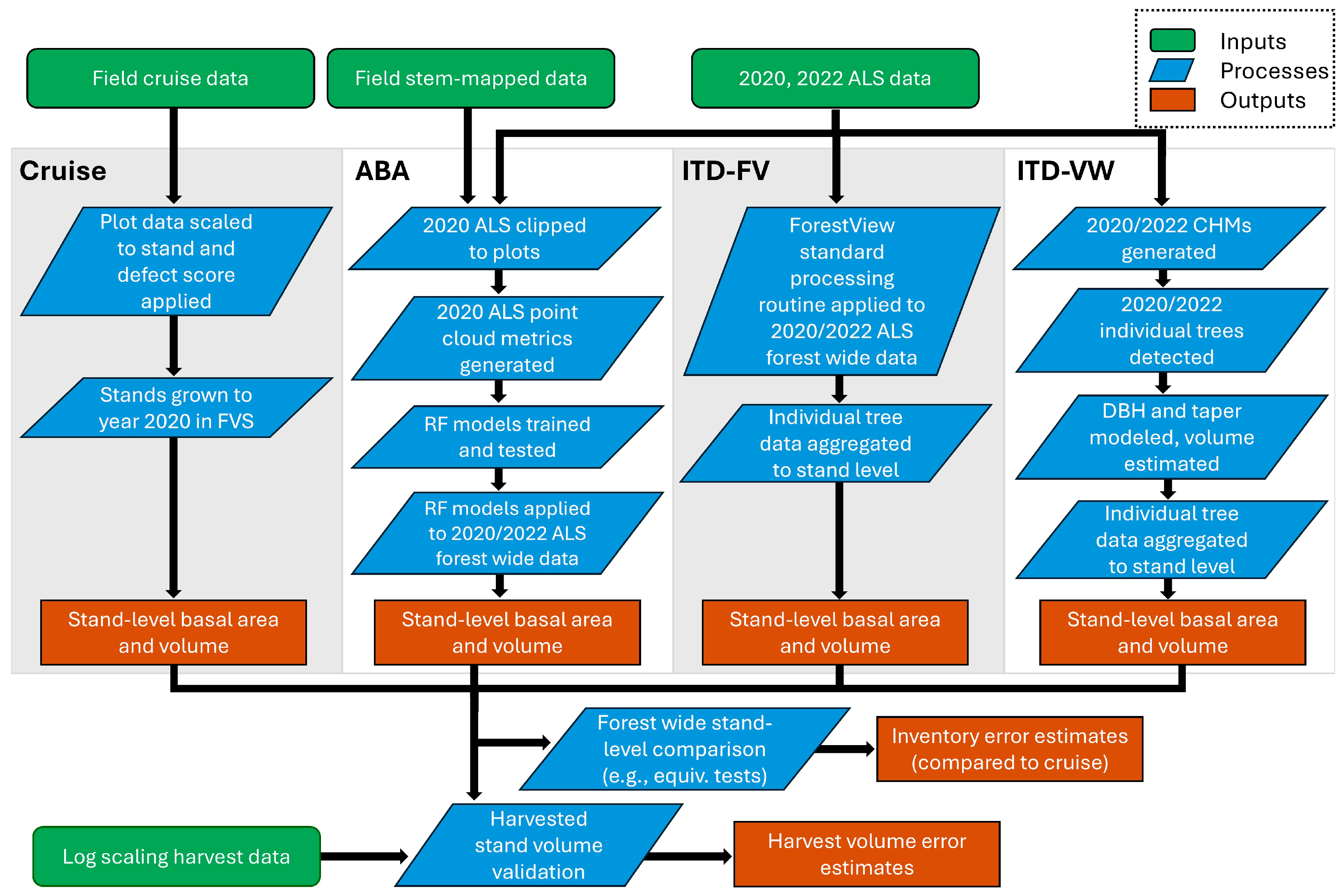
An area-based approach that used gridded summaries of the ALS point cloud and an ensemble learning algorithm to model each stand attribute at 20 m spatial resolution (hereafter referred to as ‘ABA’).

(2)

An individual tree approach that used a variable-radius local maximum filter to detect trees and then applied field-derived allometric models to estimate tree diameter at breast height (DBH) and volume (hereafter referred to as ‘ITD-VW’).

(3)

ForestView^®, a commercial ‘gray box’ method for detecting and estimating individual tree attributes (hereafter referred to as ‘ITD-FV’).

Cruise and ALS-derived total stand volume estimates were validated using the volume of harvested logs from multi-stand harvest data, tracked by load and location and scaled at the processing mill.

2. Materials and Methods

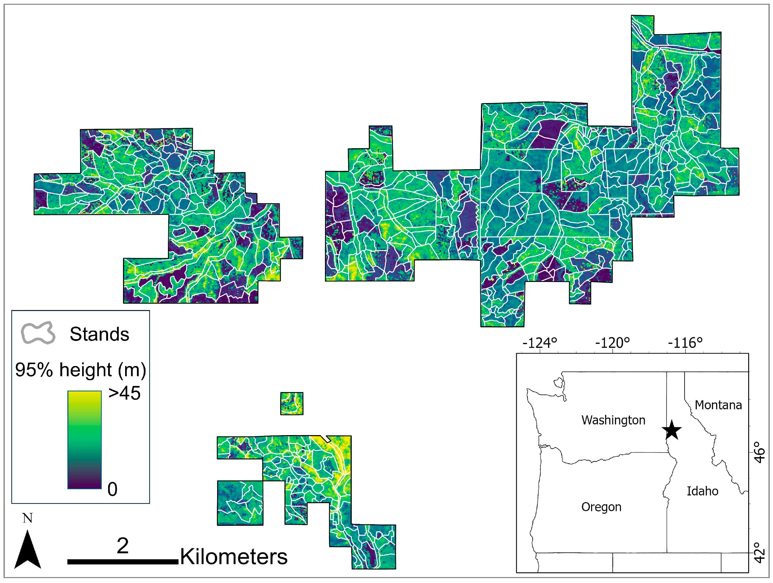
2.1. Study Area and Data

2.1.1. Study Area

This study was conducted in the University of Idaho Experimental Forest (UIEF), ~20 km north-east of Moscow, Idaho, USA (Figure 1). The UIEF is a mixed conifer, multi-use forest with a diverse range of stand structures and compositions. Stand sizes range from 0.3 to 26.7 ha across the UIEF, with an average size of 4.7 ha. Dominant species include Pseudotsuga menziesii (Mirb.) Franco var. glauca (Beissn.) Franco (Douglas fir), Abies grandis (Douglas ex D. Don) Lindl. (grand fir), Thuja plicata Donn ex D. Don (western redcedar), Larix occidentalis Nutt. (western larch), and Pinus ponderosa Dougl. ex Laws. (ponderosa pine). Other species within the study area include Pinus contorta Douglas ex Louden (lodgepole pine), Pinus monticola var. minima Lemmon (western white pine), and Picea engelmannii var. glabra Goodman (Engelmann spruce). The elevation across the UIEF ranges from ~800 to 1200 m and the local climate is characterized by cool and wet winters and warm and dry summers. Mean summer (June–August) temperature over the 1991–2020 period was 17.2 °C, mean summer precipitation was 81 mm, and mean annual precipitation was 622 mm [31].

2.1.2. Field Inventory Data: Stand-Based ‘Cruise’ Inventory

Approximately 15–20% of UIEF stands were sampled annually by supervised UIEF student forestry staff from 2013 to 2019 using a systematic random sampling approach. A 4 × 4 chain (80.48 × 80.48 m) grid was oriented on a random azimuth within each stand. The inventory used a volume-to-basal area ratio (VBAR) ‘Big-BAF’ design, with a 4.5 m² ha⁻¹ Basal Area Factor (BAF) wedge prism used to select count trees and a 15.8 m² ha⁻¹ BAF prism used to identify measure trees. The objectives of the stand-based inventory (SBI) program were to provide (1) high-quality, unit-level estimates of current standing gross and merchantable volume, stand diameter distributions, and species composition; (2) experiential learning opportunities for student staff while pursuing their forestry and other natural resources degrees; (3) field-based estimates, rather than imputed estimates, of conditions in all UIEF stands to support faculty and graduate research; (4) stand volume inputs for growth and yield projection using the Forest Vegetation Simulator (FVS) [32]; and (5) FVS-derived yield curves to update forest planning and economic analysis of management alternatives in 2020. DBHs measured using a Spencer logging tape and species were recorded for all count trees. Total height and live crown base height were measured using a TruPulse laser hypsometer (Laser Technology Inc., Centennial, CO, USA). Merchantable defects were estimated as a percentage of total gross volume to a visually estimated 15 cm top using disease- and damage-specific defect rules established for the region by Idaho Department of Lands. A 0.0013 ha fixed-area, nested regeneration plot was established at the plot center. Seedlings and saplings were tallied by species in size classes as follows: <1.37 m total height; 0–6.35 cm DBH; 6.35–12.7 cm DBH. In total, 5091 field plots were used in this analysis, with an average of 7 plots per stand. All trees from points and regeneration plots were scaled to their representative trees per hectare (tree count) in FVS tree and stand files. FVS does not explicitly accommodate VBAR/Big-BAF sampling designs. For this reason, a linear regression model was used to predict the defect severity of individual trees based on the field measured defect score, species, and stand ID. This method was used to account for widespread insect and disease damage that occurred during the 2013–2019 inventory period. Model predictions were applied to the FVS tree list file to conservatively account for insect- and disease-related damage prior to growing individual trees from the measurement year to 2020.

2.1.3. Field Inventory Data: Independent Stem-Mapped Plots

Sixty-seven 13 m fixed-radius stem-mapped forest inventory plots established in the summer of 2020 were used as reference data for the ABA. The stratified sampling strategy and plot measurements are detailed in Sparks and Smith [33] and a brief description follows. Plot location was guided by structural metrics derived from ALS point clouds and was designed to capture the variation in structure and composition across the study area. All plots were precisely located using a Triumph-2 global navigation system (JAVAD, San Jose, CA, USA) and Samsung Galaxy tablet with a Rover pole. All trees >1.5 m in height were stem-mapped using azimuth and distance from plot center and were measured for height, DBH, species, live or dead status, and canopy position (i.e., dominant, codominant, intermediate, and suppressed).

2.1.4. Airborne Laser Scanning Data and Preprocessing

Two ALS datasets were used in this study, both having complete spatial coverage of the UIEF. The first ALS dataset was acquired in September 2020 and the second was acquired in July 2022. Two ALS datasets were needed for the volume validation analysis to calculate the difference in total volume between 2020 and 2022 as the harvests were not clearcuts and standing live trees remained in each unit. Both acquisitions used a RIEGL VQ-1560II sensor (RIEGL Laser Measurement Systems, Horn, Austria) mounted on a fixed-wing aircraft with a gyro-stabilized mount. The sensor has a 58-degree field-of-view and elevation of the aircraft varied between 1600 and 1900 m above ground level to achieve a 55% flight-line overlap. The average pulse density was 20 pulses per square meter with an average per-pulse return rate over forested areas of four. Preprocessing conducted by the supplier consisted of laser intensity normalization using the RIEGL RiPROCESS software version 1.9.4 and return classification into bare earth, vegetation, water, buildings, and noise following the American Society for Photogrammetry and Remote Sensing classification standard [34]. Prior to analyses, the ALS point cloud data were converted from height above mean sea level to height above ground, using a 50 cm spatial resolution digital terrain model (DTM) interpolated from vendor-classified ground returns.

2.2. Methods

The following sections describe how the ALS inventories were derived and compared with the cruise inventory and harvest data. An overview of the methodology is outlined in Figure 2.

2.2.1. Area-Based Approach Inventory

The area-based approach used random forest modeling to estimate basal area, merchantable volume, and total volume at 20 m spatial resolution across the UIEF. Random forest is an ensemble learning algorithm that uses bootstrap samples of a reference dataset to train each tree in an ensemble of n regression or classification trees and assign a value to a response variable [35]. Random forest is a slight modification to bagged decision trees in that random forest only tries out a random subset of predictor variables (number of predictors = mtry parameter) at each decision node of the tree to identify the optimal data-split. This decorrelates the individual decision trees and often increases the performance as compared to bagged decision trees. In regression mode, the response variable is assigned the average value of the ensemble of regression trees and cross-validated against the data not included in the bootstrap samples, referred to as the out-of-bag (OOB) observations. Random forest modeling does not make distributional assumptions about the data and is insensitive to collinearity among predictor variables [35,36].

ALS data predictor metrics were calculated for each of the stem-mapped plots using the associated point clouds clipped to the plot dimensions and the ‘CloudMetrics’ program in FUSION software version 4.5 [37]. Given the small vertical errors in the DTM used to normalize the point clouds [38], only returns above 0.15 m were used in this processing step to exclude ground and near-ground returns. Canopy cover metrics were generated with a threshold of 2 m to exclude low vegetation. We selected metrics for random forest modeling (

Table 1. ALS point cloud metrics used in the random forest models. Metrics were calculated using returns above 0.15 m, unless otherwise noted.

Metric	Description
HMEAN	Height mean
HMAX	Height max
HSD	Height standard deviation
HCV	Height coefficient of variation
HSKEW	Height skewness
HKURT	Height kurtosis
H01ST	1st percentile height value
H05TH	5th percentile height value
H10TH	10th percentile height value
H20TH	20th percentile height value
H25TH	25th percentile height value
H30TH	30th percentile height value
H40TH	40th percentile height value
H50TH	50th percentile height value
H60TH	60th percentile height value
H70TH	70th percentile height value
H75TH	75th percentile height value
H80TH	80th percentile height value
H90TH	90th percentile height value
H95TH	95th percentile height value
H99TH	99th percentile height value
COV1ST	Fraction of first returns > 2 m to the total number of returns
COVALL	Fraction of all returns > 2 m to the total number of returns
COV1STMEAN	Fraction of first returns > HMEAN to the total number of returns
COVALLMEAN	Fraction of all returns > HMEAN to the total number of returns
DNS 0.15–0.5	Fraction of all returns 0.15–0.5 m to the total number of returns
DNS 0.5–1	Fraction of all returns 0.5–1 m to the total number of returns
DNS 1–2	Fraction of all returns 1–2 m to the total number of returns
DNS 2–4	Fraction of all returns 2–4 m to the total number of returns
DNS 4–8	Fraction of all returns 4–8 m to the total number of returns
DNS 8–16	Fraction of all returns 8–16 m to the total number of returns
DNS 16–32	Fraction of all returns 16–32 m to the total number of returns
DNS 32–48	Fraction of all returns 32–48 m to the total number of returns

) that have been shown to be consistently reliable predictors of basal area, volume, and biomass in prior studies (e.g., [11,13,24]).

Random forest modeling was conducted using the ‘randomForest’ R package [39] in R statistical software version 4.3.1 [40]. Separate random forest models were built for each response variable (basal area, merchantable volume, total volume) and each model used all ALS predictor metrics. This approach was used as other studies have shown that the greatest prediction accuracies are achieved when using all possible predictor variables [41]. The models were trained with n = 500 trees, and the number of variables at each split was set to the number of predictor variables divided by three. To avoid the large variability in prediction accuracy that arises by performing a single split of data into training and validation datasets, we repeatedly split the reference dataset into training and validation sets (80:20 ratio) using bootstrapping following Lyons et al. [42]. In total, 100 different sets were generated, and a model was performed using each set. Predictor variable importance was calculated as the mean squared error or the average increase in squared OOB residuals when values of the predictor variable of interest were randomly permuted in the OOB observations. The final inventory metric predictions were produced by averaging the 100 model iteration results.

Validation was performed for each model iteration using pairwise ordinary least squares (OLS) regression to quantify the relationship between each predicted response variable and the independent field validation observations. The coefficient of determination (r²), significance of the regression (p-value), and residual standard error were computed and used to evaluate the relationship ‘goodness of fit’. The results from each of the 100 iterations were used to calculate the mean and 95% confidence intervals of the accuracy statistics.

2.2.2. Local Max Filter Individual Tree Inventory (ITD-VW)

The first individual tree inventory used a generic, non-species-specific approach. A 50 cm spatial resolution canopy height model (CHM) was generated using the height-normalized point cloud following the methodology detailed in Khosravipour et al. [43]. Individual trees were then detected using a CHM-based method that uses a local max filter with a variable-radius search window filter, developed by Popescu and Wynne [44] and implemented using the ‘ForestTools’ R package in R [45]. This method passes a series of local max filters over the CHM, where the size of each local max filter is based upon the allometric relationship between tree height and tree crown diameter [crown diameter = (0.06 × height + 0.5) × 2]. This tree detection approach was used as prior studies have shown it to be one of the most accurate methods in similar mixed coniferous forests and reported lower commission errors for this approach than other local max filter methods [15].

The DBH of each detected tree was modeled using the site-appropriate height-to-DBH allometric relationship developed by Sparks et al. [30] using field data collected at 67 fixed-radius plots on the UIEF. DBH was used to estimate the basal area of each tree, and the average basal area per hectare for each stand was calculated as the sum of the basal areas for all detected trees divided by the stand area. The cubic volume of each tree was calculated using the ALS-derived height and the modeled DBH. The diameter inside the bark was estimated using the Kozak [46] taper equation from 0.3 m, assumed to be the average stump height, to the treetop in 0.5 m segments. We used regionally derived taper equation parameters [47,48] and the Smalian formula (Equation (1)) for calculating the cubic volume (V, m³) of all segments of each tree:

$$V={\displaystyle \frac{L}{2}}(A_1+A_2)$$

(1)

where L is the length of the log (m), A₁ is the area of the small end of the log (m²), and A₂ is the area of the large end of the log (m²). The total volume of each tree was calculated as the sum of the merchantable volume, or the volume of the stem where the diameter was greater than 15.24 cm, and the pulp volume, or the volume of the stem where the diameter was less than 15.24 cm but greater than 7.62 cm. All individual tree volumes were summed to the stand level for comparison with other inventory methods.

2.2.3. ForestView^® Individual Tree Inventory (ITD-FV)

The second individual tree inventory used ForestView^®, which is gray box tree detection and measurement software developed by Northwest Management Incorporated (NMI, Moscow, ID, USA); while it is described in detail elsewhere [33,49], a brief description follows. To detect individual trees, this approach iterates through several CHM-based methods, like watershed segmentation and local maximum filtering, to detect peaks in the CHM that are assumed to be treetops. Tree attributes for each detected tree are modeled using the ALS-derived structural metrics, LiDAR intensity values, and an internal database of field and ALS-measured stem mapped trees, each with species, height, DBH, crown condition, and taper information. Specifically, individual tree DBH is modeled using multivariate regression that uses the internal database, along with point cloud metrics, as predictor variables. Crown shape and structural information associated with each detected tree are used for species classification. Individual tree detection and attribution accuracies are comparable to common open access individual tree detection approaches [15]. In addition to location, height, and species, ForestView^® also provides merchantable and total volume and live or dead status. Average basal areas per hectare were calculated the same as the ITD-VW inventory. All individual tree volumes were summed to the stand level for comparison with other inventory methods.

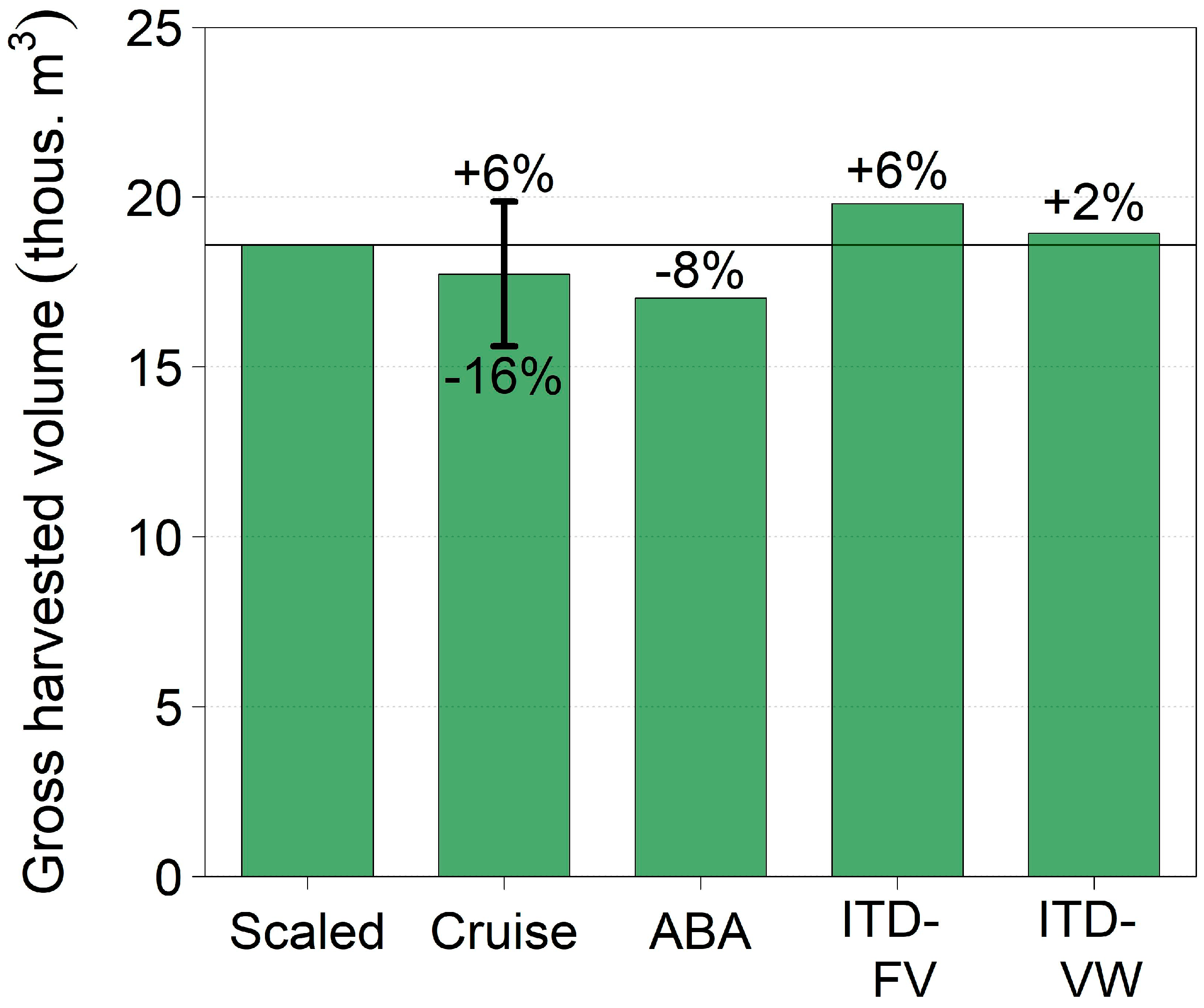
2.2.4. Validation of Inventory Volume Using Log Scaling Data

We used harvest data from three timber sales on the UIEF in 2021 that occurred between the ALS acquisitions to validate the total volume estimates provided by each inventory method. In total, ~18,588 m³ was harvested from the three harvest units between the ALS acquisitions. Out of the 763 individual log loads taken from the units, 751 were scaled at the processing mills using the Scribner decimal C log rule. This log rule estimates the number of one-inch-thick boards, spaced one-quarter inch apart, that can fit inside the circular area of a log’s smallest end. The board foot yield of this scaling cylinder can be calculated by summing the widths of each board, dividing by 12, and multiplying by the length of the log. As most logs are tapered, this method ignores volume outside the scaling cylinder and thus underestimates the volume in most logs. The volume for the remaining loads that were not scaled was estimated via a weight-to-volume conversion factor. The mill data provided gross and net board feet and species for each log load harvested from the study area. Piece count, or the number of logs on a truck, was also provided for 306 of the 763 loads.

Gross board feet were converted to cubic volume using log-diameter-dependent conversion ratios compiled by the Idaho Board of Scaling Practices [50], given the Scribner decimal C volume underestimation increases with smaller, more tapered trees [51]. We used the loads with piece count information to estimate the average diameter of logs that would fit in an average log truck, assuming triangular packing. This assumes that logs in a truck are offset from one another and not positioned directly above one another as assumed with square packing. For the loads without piece count data, we used the recommended conversion ratio for a mixed population of log sizes [50]. As the harvests were not clearcuts (e.g., <100% of stems harvested) and standing live trees remained in each unit, the difference in total volume between 2020 and 2022 for the ALS-based inventory methods was compared with the scaled reference volume. There was no post-harvest cruise data, so 2021 cruise volume estimates for the harvested stands were calculated as the sum of 2020 volume plus the FVS-modeled mean annual volume increment for each stand. To account for the partial harvest, the cruise estimates were multiplied by minimum and maximum percentage harvest values observed across the ALS-based methods to produce minimum and maximum harvested volume estimates that could be compared with the volume derived from the log scaling conducted at the processing mill. Relative volume error was calculated for each inventory method using Equation (2):

$$relative error={\displaystyle \frac{({VOL}_{INV }-{VOL}_{REF})}{{VOL}_{REF}}}\times 100$$

(2)

where VOL_INV is the inventory estimated volume and VOL_REF is the reference scaled volume for the harvested trees.

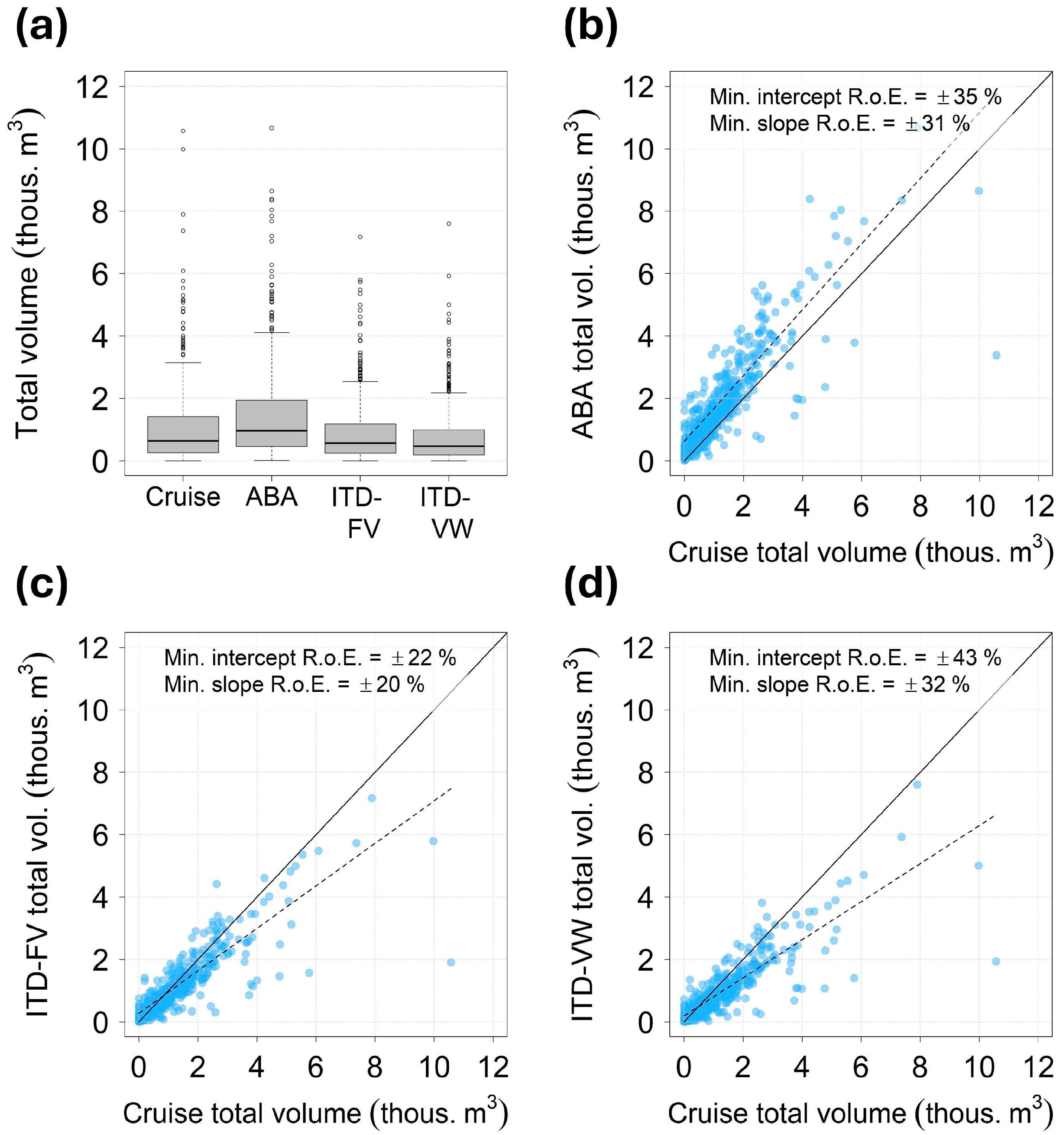
2.2.5. Comparison of Stand Inventory Methods

The equivalence of inventory methods for estimating stand metrics was assessed using regression-based equivalence tests [52]. For these tests, the null hypothesis is that the regression slope and intercept between paired sets of data are significantly different, and the alternate hypothesis is that they are not significantly different. A linear regression model is fit using the paired datasets, and an upper and a lower one-sided 95% confidence interval for both the intercept and slope is computed using the standard error regression outputs. The null hypothesis of dissimilarity is rejected if the joint one-sided 95% confidence intervals are entirely contained within a user-defined region of equivalence (e.g., ±‘X’%). Intercept equality implies the means of two datasets are not significantly different and slope equality implies that the regression slope is not significantly different from 1. Following Robinson et al. [52] and Sparks et al. [30], we report the minimum region of equivalence (R.o.E.) that would still result in the rejection of the null hypothesis of dissimilarity as this provides a less subjective approach for cross-comparing equivalence compared with arbitrarily choosing a region of equivalence. We used the cruise-derived metrics as the independent variables in the regression-based equivalence tests. Although we acknowledge that cruise-derived data do have associated measurement errors and evidence exists that ALS-derived measurements can be more accurate [28,49], cruise-derived data are commonly the standard to which other inventories are compared (e.g., [5,10,11]). The average root mean square error (RMSE) (Equation (3)) and mean bias (Equation (4)) were calculated for all inventory methods compared to the cruise-derived data as follows:

$$RMSE=\sqrt{{\displaystyle \frac{{\sum }_{i=1}^n({\widehat{x}-x_i)}^2}{n}}}$$

(3)

$$Mean bias={\displaystyle \frac{\sum _{i=1}^n(\widehat{x}-x_i)}{n}}$$

(4)

where $\widehat{x}$ is the predicted values, x_i is the observed values, and n is the number of observations. Relative RMSE (%) and bias (%) were calculated by dividing RMSE and bias by the mean observed value and multiplying by 100. Out of the 695 UIEF stands, 686 were used in the comparison given that nine stands were harvested or thinned between the cruise data and 2020 ALS acquisition. All stand-level statistics were computed using stand size weighting to account for the wide range of stand areas. Stand size weighting typically results in larger stands having a higher impact on the estimated error and is appropriate for forest inventory applications where estimates for the total amount of wood are needed [53]. All statistical analyses were conducted in R [40], and we used the ‘equivalence’ R package [54] to conduct the regression-based equivalence tests.

3. Results

3.1. Area-Based Approach Prediction Accuracy

Prediction accuracy for the basal area and volume metrics, averaged over the 100 dataset iterations, are reported in

Table 2. Statistics describing the mean values for—and relationship between—ABA-predicted and independent field validation observations, averaged over the one hundred dataset iterations. Average (±95% confidence interval) values are presented for the linear regression model coefficient of determination (r²) and associated p-value, RMSE, and mean bias.

Metric	${\overline{\mathit{x}}}_{\mathit{f}\mathit{i}\mathit{e}\mathit{l}\mathit{d}}$	${\overline{\mathit{x}}}_{\mathit{A}\mathit{B}\mathit{A}}$	r2	p	RMSE (%)	Bias (%)
Basal area (m2 ha−1)	29.7	30.9 (±0.7)	0.73 (±0.02)	0.002 (±0.004)	36.3 (±1.7)	6.1 (±2.4)
Merch. volume (m3 ha−1)	222.3	218.7 (±7.9)	0.75 (±0.03)	0.009 (±0.01)	46.2 (±3.4)	−5.6 (±2.7)
Total volume (m3 ha−1)	242.1	239.9 (±8.4)	0.76 (±0.03)	0.008 (±0.01)	42.6 (±3.4)	5.8 (±2.7)

. For basal area, the relationship between predicted and observed values had an average r² of 0.73, RMSE of 36.3%, and bias of 6.1%. The relationship between predicted and observed merchantable volume had an r² or 0.75, RMSE of 46.2%, and bias of −5.6%. The relationship between predicted and observed total volume had an r² or 0.76, RMSE of 42.6%, and bias of 5.8%.

Predictor variable importance, reported as mean decrease in accuracy, varied among the different models (Figure S1). Predictor variables ‘COVall’, ‘H50th’, ‘H30th’, ‘H10th’, and ‘DNS16-32’ were the five most important variables for predicting basal area. The five most important variables for predicting merchantable volume were ‘DNS16-32’, ‘HMEAN’, ‘H75th’, ‘H50th’, and ‘H80th’. Similarly, the five most important variables for predicting total volume were ‘DNS16-32’, ‘HMEAN’, ‘H40th’, ‘H50th’, and ‘H75th’.

3.2. Validation of Harvested Volume

The gross harvested total volume estimated by each inventory method is shown in Figure 3. The gross harvested total volume scaled at the processing mills was 18,588 m³. The harvested volume estimates derived from the cruise (17,738 ± 1951 m³) and ABA (17,026 m³) inventory methods were 5 (±11%) and 8% lower than the reference scaled volume, respectively. The harvested volume estimates from ITD-FV (19,815 m³) and ITD-VW (18,933 m³) were 6% and 2% greater than the reference scaled volume, respectively.

3.3. Comparison of Forest-Wide Inventories

The distribution of UIEF stand basal area estimated by each inventory method is shown in Figure 4a and regression-based equivalence tests for cruise-estimated basal area compared with the other three methods are shown in Figure 4b–d. The linear relationship between cruise-estimated basal area and the individual tree inventory estimates had lower r² and higher RMSE than the relationship between the ABA inventory and the cruise inventory (

Table 3. Statistics describing the relationship between cruise- and ALS-estimated stand-level inventory metrics. For each relationship, the linear regression model coefficient of determination (r²) and associated p-value, RMSE, and mean bias are reported.

Metric	Inventory	r2	p	RMSE (%)	Bias (%)
Basal area	ABA	0.32	<0.001	76.6	12.5
	ITD-FV	0.31	<0.001	78.7	−16.9
	ITD-VW	0.31	<0.001	84.2	−33.4
Merchantable volume	ABA	0.85	<0.001	115.2	82.8
	ITD-FV	0.85	<0.001	37.9	−3.0
	ITD-VW	0.84	<0.001	39.7	−4.5
Total volume	ABA	0.77	<0.001	74.8	45.3
	ITD-FV	0.78	<0.001	51.9	−14.3
	ITD-VW	0.77	<0.001	59.3	−26.8

). The regression-based intercept and slope equivalence with the cruise-estimated basal area varied among the methods with the ABA-derived basal area having the lowest region of equivalence for both the intercept (±17% or greater) and slope (±17% or greater) (Figure 4b).

Different trends were observed between cruise-derived merchantable and total volume and other inventory merchantable and total volume (Figure 5 and Figure 6). In general, the linear relationship between cruise-estimated merchantable and total volume and the individual tree inventory estimates had lower RMSE and bias than the relationship between ABA and cruise volume estimates (Table 3). The regression-based intercept and slope equivalence with the cruise-estimated merchantable volume varied among the methods, but the ITD-FV merchantable volume had the lowest region of equivalence for both the intercept (±7% or greater) and the slope (±10% or greater) (Figure 5c). Likewise, regions of equivalence between cruise-estimated total volume and the ITD-FV inventory total volume were smaller (intercept R.o.E.: ±22% or greater; slope R.o.E.: ±20% or greater) than the ABA inventory (intercept R.o.E.: ±35% or greater; slope R.o.E.: ±31% or greater) (Figure 6b) and the ITD-VW inventory (intercept R.o.E.: ±43% or greater; slope R.o.E.: ±32% or greater) (Figure 6d).

4. Discussion

Forest managers need information from accurate forest inventories, aggregated to the stand scale, to make operational decisions and model growth and yield. This study compared stand-level forest inventories derived from a conventional stand-based inventory and ALS area-based and individual tree approaches. Cruise- and ALS-derived total volume estimates were validated using multi-stand harvest data where harvested logs were tracked by load and location and scaled at the processing mills. In terms of total harvested volume, the ABA and individual tree methods had similar error (−8 to 6%) to the cruise estimate (−16 to 6%) when compared with scaled volume. These results suggest that high-pulse-density (e.g., ≥20 ppm) ALS-based inventories may be preferred in similar forests where spatially complete inventories are needed as they meet the reported manager-preferred error threshold of 10% or less [8,9]. However, as this study was undertaken in a single mixed conifer forest, these findings may have limited applicability to other forest types or climatic regions. While accurate stand-level information is important, managers also need to consider the within-stand information that ALS data can provide. For example, the location of within-stand tree volume and species is useful information for scheduling and organizing product flow to reduce harvesting and hauling costs and facilitate growth modeling and silvicultural treatment planning [6,7].

The findings of this study and others show that contemporary ALS-derived inventories can provide accurate stand-level estimates of volume that are comparable to or better than conventional sample-based inventories. Other studies have observed lower error from ALS-derived volume estimates than field-estimated volume and that using field data to validate ALS inventories can limit the accuracy of the ALS inventory [28]. Validating stand-level attributes, such as stem volume, is a significant challenge due to the resources needed to measure every tree, except in smaller stands where a census can be completed (e.g., [30]). The ability of contemporary harvesting equipment to record stem size and length as trees are harvested [24] offers a significant and largely untapped resource for validating ALS-based inventories. However, high equipment maintenance costs and inaccurate measurement sensors and algorithms could preclude the use of these data in many circumstances. Other studies have used weight scaling and log scaling data to validate ALS-derived volume. Both Woods et al. [6] and White et al. [29] observed less than 10% error in ALS-derived volume compared to weight and log scaling data. This error level is similar to that observed in this study, where ALS-based inventories were within 8% of scaled volume. Sparks et al. [30] observed 1%–29% underestimation in ALS-derived individual tree inventory volume compared to log scaling data, although increased error due to difficulties in tracking individual log loads was reported. The use of log scaling data as an independent validation dataset for ALS-derived volume is promising; however, there is an unknown amount of error associated with converting scaled volume to cubic volume [30]. Future studies could quantify this error by comparing volume estimates for stands where there are both direct harvester measurements and log scaling data available.

Cruise- and ALS-derived individual tree-estimated stand volume was consistently lower than the ABA estimated stand volume (Figure 5 and Figure 6). Volume underestimation in individual tree inventories is well documented given that contemporary individual tree detection methods are prone to under detection of trees [16,30,33,55,56]. There are several potential reasons why the cruise-derived inventory produced lower volume estimates compared to the ABA inventory. First, and most importantly, the stand-based inventory data were collected over a 6-year period (2013–2019) preceding the common year used for comparison (2020). All harvested stands used for volume validation were among the first sampled at the beginning of the inventory cycle in 2013, and thus likely had the greatest error in their projection of growth between 2013 and 2020. While we lacked the data to quantify this error, other studies in mixed conifer forests have found that differences between field-measured and FVS-projected growth over relatively short time periods (e.g., <10 years) are typically less than 10% [57]. Second, the harvested stands used in this analysis had some damage, including mortality, associated with insect and disease issues during the period 2013–2020. The UIEF stand-based inventory predicted individual tree volumes adjusted for measured tree defects by species and individual stand prior to stand growth projection. This adjustment to the FVS individual tree list used for growth simulation likely contributed to an underestimation of overall stand gross volume. Finally, it is important to note that forest attribute quantification using ABA and ITD methods is highly dependent on the method type and parameterization [15,20]. While we employed several common ABA and ITD approaches, different methods would likely influence the similarity of the produced inventories.

An additional driver of differences between cruise- and ALS-based estimates is that many of the stands in the UIEF do not have a uniform distribution of trees within the stand due to partial harvesting practices. The topography and location of standing volume within each stand dictate how logging roads and landings are constructed. Consequently, many stands may be partially harvested and, depending on the field sampling plot locations, residual timber may be mostly or completely omitted in subsequent plot revisits. An increased sampling intensity may better capture volume in these non-uniform stands; however, this would increase the time and resource costs associated with measuring more field plots. Historically, external timber sale auctions conducted by the UIEF have received a more detailed product cruise prior to appraisal to increase the accuracy of an inventory immediately prior to harvest. Many state and industrial landowners have similar pre-harvest practices as well as distinct methods for long-term stand-based inventory programs that support forest planning and timber sale activity. In this study, a detailed product cruise was not completed immediately prior to harvesting because wood from the harvest units was associated with a capital mass timber building project on the University of Idaho campus and not a public auction. A more detailed product cruise with increased sampling intensity conducted immediately prior to harvest would likely have yielded lower error estimates.

While accurate estimates of forest attributes are needed by forest managers at the stand level, an important difference between conventional cruise inventories and ALS-derived inventories is the spatial variability of those attributes within stands that ALS-derived inventories provide. For example, the intra-stand information in ALS-derived inventories can help with harvest planning, including identifying ‘cut’ and ‘leave’ trees, as well as road and log landing construction [6,7]. In some cases where stands have homogenous species composition and structure, such as plantations, this information may be less useful. However, in highly heterogeneous stands typical of North American mixed conifer forests, these data can provide useful spatial information at a variety of different levels, from coarse gridded data to individual trees characterized by volume and species. For example, the classification of individual tree species provided by some ITD methods (e.g., ForestView^®) is important for planning and estimating harvest revenue, given the value of different species varies widely [7]. However, accurate species classification remains a limitation of most ALS-derived inventories [2,4], which may make these inventories less useful for managers that need species-level information. An additional important, and understudied, consideration of ALS-derived wall-to-wall inventories is the spatial distribution of estimated volume error due to varying terrain and canopy structure. While this study lacked sufficient data to quantify these errors, future studies could explore this aspect to provide value-added products to forest managers.

In dynamic, mixed species forests, insect and disease impacts occur intermittently, and repeat ALS-based inventories could provide complementary data to conventional, sample-based inventory (cruise) programs by capturing spatially explicit mortality and expressed growth of individual trees matched between ALS datasets. The cruise-based inventory in this study used growth and mortality model projection over periods of up to six years and did not capture the intermittent mortality due to insects and disease. ALS-based estimates provide a high level of certainty in what exists on a forested landscape at a fixed, specific point in time when flights occur, but it is not well understood how often ALS-based assessments are needed to accurately quantify individual and stand-level change [58]. For example, some studies have found that several years are needed between ALS acquisitions for the height growth to exceed the uncertainty in the height estimates [59]. Regardless of the ALS acquisition frequency, field data will undoubtedly remain a critical tool for updating inventories in between ALS acquisitions, calibrating ALS-derived models, and validating ALS-derived inventories [4,58,60]. The potential to leverage Digital Aerial Photogrammetric (DAP) point clouds derived from stereo imagery to monitor change following an ALS collection shows some promise and should be a focus of future research. For example, the segmentation of NAIP-derived canopy height models could potentially supplement current ALS acquisitions, given its ability to quantify stand height [61,62], and its relatively high acquisition frequency of 2–3 years for the entire conterminous United States.

5. Conclusions

This study advances our understanding of field- and ALS-derived stand-level inventory errors, and identifies some practical considerations associated with cruise versus ALS-based inventories, in a structure- and species-diverse mixed conifer forest. Our results show that the ALS-derived area-based and individual tree approaches had similar errors (−8 to 6%) to the cruise estimate (−16 to 6%) when compared with scaled volume, indicating that ALS-based methods may be preferred by forest managers that need complete spatial coverage of forest stands. Depending on the application, certain ALS-based approaches may be more suitable than others, as evidenced by the conservative volume estimates provided by ALS-derived individual tree approaches. Area-based approaches may also provide more accurate information on the non-merchantable stand components (e.g., non-dominant trees), which are important for growth and yield modeling, given the known under detection of non-dominant trees by ITD approaches. However, in forests or plantations that have lower structure and species variability, individual tree methods may provide estimates of stand volume that are more similar to field-based and other ALS-based approaches. Our results also highlight the spatially explicit information provided by gridded and individual tree ALS-derived inventories. Research is needed to understand how this spatial information impacts forest operations and management decisions including scheduling and organizing product flow to reduce harvesting and hauling costs, conducting growth modeling, and planning silvicultural treatment. Our findings, coupled with those of other studies, suggest that in heterogenous forests ALS-derived stand-level volume validation should be completed with wall-to-wall independent data, such as census-level field measurements, log scaling data, or harvester measurements.

References

1. Tinkham, W.T.; Mahoney, P.R.; Hudak, A.T.; Domke, G.M.; Falkowski, M.J.; Woodall, C.W.; Smith, A.M.S. Applications of the United States Forest Inventory and Analysis dataset: A review and future directions. Can. J. For. Res. 2018, 48, 1251–1268. [Google Scholar] [CrossRef]
2. Maltamo, M.; Packalen, P.; Kangas, A. From comprehensive field inventories to remotely sensed wall-to-wall stand attribute data—A brief history of management inventories in the Nordic countries. Can. J. For. Res. 2021, 51, 257–266. [Google Scholar] [CrossRef]
3. Frayer, W.E.; Furnival, G.M. History of Forest Survey Sampling Designs in the United States. In Integrated Tools for Natural Resources Inventories in the 21st Century; Hansen, M., Burk, T., Eds.; Gen. Tech. Rep. NC-212; USDA Forest Service, North Central Forest Experiment Station: St. Paul, MN, USA, 2000; pp. 42–49. [Google Scholar]
4. White, J.C.; Coops, N.C.; Wulder, M.A.; Vastaranta, M.; Hilker, T.; Tompalski, P. Remote sensing technologies for enhancing forest inventories: A review. Can. J. Remote Sens. 2016, 42, 619–641. [Google Scholar] [CrossRef]
5. Hemingway, H.; Opalach, D. Integrating Lidar Canopy Height Models with Satellite-Assisted Inventory Methods: A Comparison of Inventory Estimates. For. Sci. 2024, 70, 2–13. [Google Scholar] [CrossRef]
6. Woods, M.; Pitt, D.; Penner, M.; Lim, K.; Nesbitt, D.; Etheridge, D.; Treitz, P. Operational implementation of a LiDAR inventory in Boreal Ontario. For. Chron. 2011, 87, 512–528. [Google Scholar] [CrossRef]
7. Keefe, R.F.; Zimbelman, E.G.; Picchi, G. Use of individual tree and product level data to improve operational forestry. Curr. For. Rep. 2022, 8, 148–165. [Google Scholar] [CrossRef]
8. Meddens, A.J.; Steen-Adams, M.M.; Hudak, A.T.; Mauro, F.; Byassee, P.M.; Strunk, J. Specifying geospatial data product characteristics for forest and fuel management applications. Environ. Res. Lett. 2022, 17, 045025. [Google Scholar] [CrossRef]
9. Fassnacht, F.E.; Mager, C.; Waser, L.T.; Kanjir, U.; Schäfer, J.; Buhvald, A.P.; Shafeian, E.; Schiefer, F.; Stančič, L.; Immitzer, M.; et al. Forest practitioners’ requirements for remote sensing-based canopy height, wood-volume, tree species, and disturbance products. For. Int. J. For. Res. 2024, 98, 233–252. [Google Scholar] [CrossRef]
10. Hummel, S.; Hudak, A.T.; Uebler, E.H.; Falkowski, M.J.; Megown, K.A. A comparison of accuracy and cost of LiDAR versus stand exam data for landscape management on the Malheur National Forest. J. For. 2011, 109, 267–273. [Google Scholar] [CrossRef]
11. Hayashi, R.; Weiskittel, A.; Kershaw, J.A., Jr. Influence of prediction cell size on LiDAR-derived area-based estimates of total volume in mixed-species and multicohort forests in northeastern North America. Can. J. Remote Sens. 2016, 42, 473–488. [Google Scholar] [CrossRef]
12. Næsset, E. Predicting forest stand characteristics with airborne scanning laser using a practical two-stage procedure and field data. Remote Sens. Environ. 2002, 80, 88–99. [Google Scholar] [CrossRef]
13. Silva, C.A.; Hudak, A.T.; Klauberg, C.; Vierling, L.A.; Gonzalez-Benecke, C.; de Padua Chaves Carvalho, S.; Rodriguez, L.C.E.; Cardil, A. Combined effect of pulse density and grid cell size on predicting and mapping aboveground carbon in fast-growing Eucalyptus forest plantation using airborne LiDAR data. Carbon Bal. Manag. 2017, 12, 13. [Google Scholar] [CrossRef] [PubMed]
14. Falkowski, M.J.; Smith, A.M.S.; Gessler, P.E.; Hudak, A.T.; Vierling, L.A.; Evans, J.S. The influence of conifer forest canopy cover on the accuracy of two individual tree measurement algorithms using lidar data. Can. J. Remote Sens. 2008, 34, S338–S350. [Google Scholar] [CrossRef]
15. Sparks, A.M.; Corrao, M.V.; Smith, A.M.S. Cross-comparison of individual tree detection methods using low and high pulse density airborne laser scanning data. Remote Sens. 2022, 14, 3480. [Google Scholar] [CrossRef]
16. Vastaranta, M.; Holopainen, M.; Yu, X.; Hyyppä, J.; Mäkinen, A.; Rasinmäki, J.; Melkas, T.; Kaartinen, H.; Hyyppä, H. Effects of individual tree detection error sources on forest management planning calculations. Remote Sens. 2011, 3, 1614–1626. [Google Scholar] [CrossRef]
17. Soininen, V.; Kukko, A.; Yu, X.; Kaartinen, H.; Luoma, V.; Saikkonen, O.; Holopainen, M.; Matikainen, L.; Lehtomäki, M.; Hyyppä, J. Predicting growth of individual trees directly and indirectly using 20-year bitemporal airborne laser scanning point cloud data. Forests 2022, 13, 2040. [Google Scholar] [CrossRef]
18. Fassnacht, F.E.; White, J.C.; Wulder, M.A.; Næsset, E. Remote sensing in forestry: Current challenges, considerations and directions. For. Int. J. For. Res. 2024, 97, 11–37. [Google Scholar] [CrossRef]
19. Peuhkurinen, J.; Mehtätalo, L.; Maltamo, M. Comparing individual tree detection and the area-based statistical approach for the retrieval of forest stand characteristics using airborne laser scanning in Scots pine stands. Can. J. For. Res. 2011, 41, 583–598. [Google Scholar] [CrossRef]
20. Frank, B.; Mauro, F.; Temesgen, H. Model-based estimation of forest inventory attributes using lidar: A comparison of the area-based and semi-individual tree crown approaches. Remote Sens. 2020, 12, 2525. [Google Scholar] [CrossRef]
21. Vieira Leite, R.; Hummel do Amaral, C.; De Paula Pires, R.; Silva, C.A.; Boechat Soares, C.P.; Paulo Macedo, R.; Araújo Lopes Da Silva, A.; North Broadbent, E.; Mohan, M.; Garcia Leite, H. Estimating Stem Volume in Eucalyptus Plantations Using Airborne LiDAR: A Comparison of Area-and Individual Tree-Based Approaches. Remote Sens. 2020, 12, 1513. [Google Scholar] [CrossRef]
22. Yu, X.; Hyyppä, J.; Holopainen, M.; Vastaranta, M. Comparison of area-based and individual tree-based methods for predicting plot-level forest attributes. Remote Sens. 2010, 2, 1481–1495. [Google Scholar] [CrossRef]
23. Lara-Gómez, M.Á.; Navarro-Cerrillo, R.M.; Clavero Rumbao, I.; Palacios-Rodríguez, G. Comparison of errors produced by ABA and ITC methods for the estimation of forest inventory attributes at stand and tree level in Pinus radiata plantations in Chile. Remote Sens. 2023, 15, 1544. [Google Scholar] [CrossRef]
24. White, J.C.; Wulder, M.A.; Varhola, A.; Vastaranta, M.; Coops, N.C.; Cook, B.D.; Pitt, D.; Woods, M. A best practices guide for generating forest inventory attributes from airborne laser scanning data using an area-based approach. For. Chron. 2013, 89, 722–723. [Google Scholar] [CrossRef]
25. Peuhkurinen, J.; Maltamo, M.; Malinen, J.; Pitkänen, J.; Packalén, P. Preharvest measurement of marked stands using airborne laser scanning. For. Sci. 2007, 53, 653–661. [Google Scholar] [CrossRef]
26. Korhonen, L.; Peuhkurinen, J.; Malinen, J.; Suvanto, A.; Maltamo, M.; Packalen, P.; Kangas, J. The use of airborne laser scanning to estimate sawlog volumes. Forestry 2008, 81, 499–510. [Google Scholar]
27. Holopainen, M.; Vastaranta, M.; Rasinmäki, J.; Kalliovirta, J.; Mäkinen, A.; Haapanen, R.; Melkas, T.; Yu, X.; Hyyppä, J. Uncertainty in timber assortment estimates predicted from forest inventory data. Eur. J. For. Res. 2010, 129, 1131–1142. [Google Scholar] [CrossRef]
28. Persson, H.J.; Olofsson, K.; Holmgren, J. Two-phase forest inventory using very-high-resolution laser scanning. Remote Sens. Environ. 2022, 271, 112909. [Google Scholar] [CrossRef]
29. White, J.C.; Wulder, M.A.; Buckmaster, G. Validating estimates of merchantable volume from airborne laser scanning (ALS) data using weight scale data. For. Chron. 2014, 90, 378–385. [Google Scholar] [CrossRef]
30. Sparks, A.M.; Corrao, M.V.; Keefe, R.F.; Armstrong, R.; Smith, A.M.S. An Accuracy Assessment of Field and Airborne Laser Scanning–Derived Individual Tree Inventories using Felled Tree Measurements and Log Scaling Data in a Mixed Conifer Forest. For. Sci. 2024, 70, 228–241. [Google Scholar] [CrossRef]
31. NOAA. NOAA’s US Climate Normals (1991–2020). NOAA National Centers for Environmental Information; 2022. Available online: https://www.ncei.noaa.gov/products/land-based-station/us-climate-normals (accessed on 11 December 2024).
32. Dixon, G.E. Essential FVS: A User’s Guide to the Forest Vegetation Simulator; USDA Forest Service, Forest Management Service Center: Fort Collins, CO, USA, 2002.
33. Sparks, A.M.; Smith, A.M.S. Accuracy of a lidar-based individual tree detection and attribute measurement algorithm developed to inform forest products supply chain and resource management. Forests 2021, 13, 3. [Google Scholar] [CrossRef]
34. ASPRS. ASPRS LAS Format Standard 1.4. 2019. Available online: https://www.asprs.org/wp-content/uploads/2019/07/LAS_1_4_r15.pdf (accessed on 9 December 2024).
35. Breiman, L. Random forests. Mach. Learn. 2001, 45, 5–32. [Google Scholar] [CrossRef]
36. Cutler, D.R.; Edwards Jr, T.C.; Beard, K.H.; Cutler, A.; Hess, K.T.; Gibson, J.; Lawler, J.J. Random forests for classification in ecology. Ecology 2007, 88, 2783–2792. [Google Scholar] [CrossRef] [PubMed]
37. McGaughey, R.J. FUSION/LDV: Software for LIDAR Data Analysis and Visualization; USDA Forest Service, Pacific Northwest Research Station: Seattle, WA, USA, 2024. Available online: http://forsys.cfr.washington.edu/fusion/fusion_overview.html (accessed on 29 November 2024).
38. Tinkham, W.T.; Smith, A.M.S.; Hoffman, C.; Hudak, A.T.; Falkowski, M.J.; Swanson, M.E.; Gessler, P.E. Investigating the influence of LiDAR ground surface errors on the utility of derived forest inventories. Can. J. For. Res. 2012, 42, 413–422. [Google Scholar] [CrossRef]
39. Liaw, A.; Wiener, M. Classification and Regression by randomforest. R News 2002, 2, 18–22. [Google Scholar]
40. R Core Team. R: A Language and Environment for Statistical Computing; R Foundation for Statistical Computing: Vienna, Austria, 2024. [Google Scholar]
41. Collins, L.; McCarthy, G.; Mellor, A.; Newell, G.; Smith, L. Training data requirements for fire severity mapping using Landsat imagery and random forest. Remote Sens. Environ. 2020, 245, 111839. [Google Scholar] [CrossRef]
42. Lyons, M.B.; Keith, D.A.; Phinn, S.R.; Mason, T.J.; Elith, J. A comparison of resampling methods for remote sensing classification and accuracy assessment. Remote Sens. Environ. 2018, 208, 145–153. [Google Scholar] [CrossRef]
43. Khosravipour, A.; Skidmore, A.K.; Isenburg, M.; Wang, T.; Hussin, Y.A. Generating pit-free canopy height models from airborne lidar. Photogramm. Eng. Remote Sens. 2014, 80, 863–872. [Google Scholar] [CrossRef]
44. Popescu, S.C.; Wynne, R.H. Seeing the trees in the forest. Photogramm. Eng. Remote Sens. 2004, 70, 589–604. [Google Scholar] [CrossRef]
45. Plowright, A.; Roussel, J. ForestTools: Tools for Analyzing Remote Sensing Forest Data. R Package Version 1.0.2. 2023. Available online: https://github.com/andrew-plowright/ForestTools (accessed on 20 October 2024).
46. Kozak, A. My last words on taper equations. For. Chron. 2004, 80, 507–515. [Google Scholar] [CrossRef]
47. Pancoast, A.D. Evaluation of Taper and Volume Estimation Techniques for Ponderosa Pine in Eastern Oregon and Eastern Washington. Master’s Thesis, Oregon State University, Corvallis, OR, USA, 2018. [Google Scholar]
48. Poudel, K.P.; Temesgen, H.; Gray, A.N. Estimating upper stem diameters and volume of Douglas-fir and Western hemlock trees in the Pacific northwest. For. Ecosyst. 2018, 5, 16. [Google Scholar] [CrossRef]
49. Corrao, M.V.; Sparks, A.M.; Smith, A.M.S. A Conventional Cruise and Felled-Tree Validation of Individual Tree Diameter, Height and Volume Derived from Airborne Laser Scanning Data of a Loblolly Pine (P. taeda) Stand in Eastern Texas. Remote Sens. 2022, 14, 2567. [Google Scholar] [CrossRef]
50. Idaho Board of Scaling Practices. Basic Information About Cubic Scaling. 2018. Available online: https://ibsp.idaho.gov/wp-content/uploads/2018/06/BASIC-INFORMATION-ABOUT-CUBIC-SCALING.pdf (accessed on 7 March 2024).
51. Spelter, H. Converting among log scaling methods: Scribner, International, and Doyle versus cubic. J. For. 2004, 102, 33–39. [Google Scholar] [CrossRef]
52. Robinson, A.P.; Duursma, R.A.; Marshall, J.D. A regression-based equivalence test for model validation: Shifting the burden of proof. Tree Phys. 2005, 25, 903–913. [Google Scholar] [CrossRef] [PubMed]
53. Hyyppa, H.J.; Hyyppa, J.M. Effects of stand size on the accuracy of remote sensing-based forest inventory. IEEE Trans. Geosci. Remote Sens. 2001, 39, 2613–2621. [Google Scholar] [CrossRef]
54. Robinson, A. Equivalence: Provides Tests and Graphics for Assessing Tests of Equivalence, Version 0.7.2. Available online: https://cran.r-project.org/web/packages/equivalence/ (accessed on 23 January 2024).
55. Wang, Y.; Hyyppä, J.; Liang, X.; Kaartinen, H.; Yu, X.; Lindberg, E.; Holmgren, J.; Qin, Y.; Mallet, C.; Ferraz, A.; et al. International benchmarking of the individual tree detection methods for modeling 3-D canopy structure for silviculture and forest ecology using airborne laser scanning. IEEE Trans. Geosci. Remote Sens. 2016, 54, 5011–5027. [Google Scholar] [CrossRef]
56. Wielgosz, M.; Puliti, S.; Xiang, B.; Schindler, K.; Astrup, R. SegmentAnyTree: A sensor and platform agnostic deep learning model for tree segmentation using laser scanning data. Remote Sens. Environ. 2024, 313, 114367. [Google Scholar] [CrossRef]
57. Herbert, C.; Fried, J.S.; Butsic, V. Validation of Forest vegetation simulator model finds overprediction of carbon growth in California. Forests 2023, 14, 604. [Google Scholar] [CrossRef]
58. Tompalski, P.; Coops, N.C.; White, J.C.; Goodbody, T.R.; Hennigar, C.R.; Wulder, M.A.; Socha, J.; Woods, M.E. Estimating changes in forest attributes and enhancing growth projections: A review of existing approaches and future directions using airborne 3D point cloud data. Curr. For. Rep. 2021, 7, 1–24. [Google Scholar] [CrossRef]
59. Hopkinson, C.; Chasmer, L.; Hall, R.J. The uncertainty in conifer plantation growth prediction from multi-temporal lidar datasets. Remote Sens. Environ. 2008, 112, 1168–1180. [Google Scholar] [CrossRef]
60. Coops, N.C.; Tompalski, P.; Goodbody, T.R.; Achim, A.; Mulverhill, C. Framework for near real-time forest inventory using multi source remote sensing data. Forestry 2023, 96, 1–19. [Google Scholar] [CrossRef]
61. Strunk, J.; Packalen, P.; Gould, P.; Gatziolis, D.; Maki, C.; Andersen, H.E.; McGaughey, R.J. Large area forest yield estimation with pushbroom digital aerial photogrammetry. Forests 2019, 10, 397. [Google Scholar] [CrossRef]
62. Ritz, A.L.; Thomas, V.A.; Wynne, R.H.; Green, P.C.; Schroeder, T.A.; Albaugh, T.J.; Burkhart, H.E.; Carter, D.R.; Cook, R.L.; Campoe, O.C.; et al. Assessing the utility of NAIP digital aerial photogrammetric point clouds for estimating canopy height of managed loblolly pine plantations in the southeastern United States. Int. J. Appl. Earth Obs. Geoinf. 2022, 113, 103012. [Google Scholar] [CrossRef]
Figure 1. Overview and location of the University of Idaho Experimental Forest in north-central Idaho, USA. An ALS-derived 20 m spatial resolution height map for the year 2020 showing the 95th percentile height in each cell is shown to illustrate the structural variability within and among stands. Forest stand boundaries are overlaid in white.
Forests 16 00784 g001
Figure 2. Study framework highlighting inputs, processes, and outputs involved with the forest-wide inventory comparison and harvested stand validation. Stand inventories include the following: Cruise: cruise-based inventory; ABA: area-based approach inventory; ITD-FV: ForestView individual tree inventory; and ITD-VW: local max filter individual tree inventory. Abbreviations: ALS: airborne laser scanning; FVS: Forest Vegetation Simulator; RF: random forest; CHM: canopy height model; DBH: diameter at breast height.
Forests 16 00784 g002
Figure 3. Comparison of gross harvested total volume in thousand cubic meters derived from the scaled data, forest-wide cruise data (‘Cruise’), area-based approach (ABA), ForestView® (ITD-FV), and variable-radius window filter (ITD-VW) individual tree inventories. The cruise volume error bar represents the estimated range of volume due to uncertainty in the proportion of residual stems in the harvest units.
Forests 16 00784 g003
Figure 4. The distribution of stand-level basal area (m2 ha−1) estimated by the four inventory methods (a). Regression-based equivalence tests between the cruise-estimated and (b) area-based approach (ABA)-estimated basal area, (c) ForestView® individual tree inventory (ITD-FV)-estimated basal area, and (d) variable-radius window filter individual tree inventory (ITD-VW)-estimated basal area. In all subplots, each dot represents one of the 686 analyzed UIEF stands. The dotted line represents the best-fit linear regression model, and the solid black line represents the 1:1 line. The reported minimum regions of equivalence (R.o.E.) for the intercept and slope were calculated with the independent variable on the y-axis as required by the ‘equivalence’ package, but here the independent variable is shown on the x-axis to be consistent with general linear regression plotting practices.
Forests 16 00784 g004
Figure 5. The distribution of stand-level merchantable volume (thousand m3) estimated by the four inventory methods (a). Regression-based equivalence tests between the cruise-estimated and (b) the area-based approach (ABA)-estimated merchantable volume, (c) ForestView® individual tree inventory (ITD-FV)-estimated merchantable volume, and (d) variable-radius window filter individual tree inventory (ITD-VW)-estimated merchantable volume. In all subplots, each dot represents one of the 686 analyzed UIEF stands. The dotted line represents the best-fit linear regression model, and the solid black line represents the 1:1 line. The reported minimum regions of equivalence (R.o.E.) for the intercept and slope were calculated with the independent variable on the y-axis as required by the ‘equivalence’ package, but here the independent variable is shown on the x-axis to be consistent with general linear regression plotting practices.
Forests 16 00784 g005
Figure 6. The distribution of stand-level total volume (thousand m3) estimated by the four inventory methods (a). Regression-based equivalence tests between the cruise-estimated and (b) the area-based approach (ABA)-estimated total volume, (c) ForestView® individual tree inventory (ITD-FV)-estimated total volume, and (d) variable-radius window filter individual tree inventory (ITD-VW)-estimated total volume. In all subplots, each dot represents one of the 686 analyzed UIEF stands. The dotted line represents the best-fit linear regression model, and the solid black line represents the 1:1 line. The reported minimum regions of equivalence (R.o.E.) for the intercept and slope were calculated with the independent variable on the y-axis as required by the ‘equivalence’ package, but here the independent variable is shown on the x-axis to be consistent with general linear regression plotting practices.
Forests 16 00784 g006