Simulation-Based Correction of Geolocation Errors in GEDI Footprint Positions Using Monte Carlo Approach

Abstract

Traditional remote sensing techniques face notable limitations in accurately estimating forest canopy height. Optical data often suffer from vegetation occlusion, while radar systems, though capable of penetrating foliage, show reduced accuracy in complex terrains. The Global Ecosystem Dynamics Investigation (GEDI), a spaceborne LiDAR mission, offers high-resolution measurements that address these challenges. However, the complexity of waveform processing and the influence of geolocation uncertainty demand rigorous assessment. This study employs GEDI Version 2.0 data, which demonstrates substantial improvement in geolocation accuracy compared to Version 1.0, and integrates airborne laser scanning (ALS) data from the Changbai Mountain forest region to simulate GEDI waveforms. A Monte Carlo-based approach was used to quantify and correct geolocation offsets, resulting in a reduction in the average relative error (defined as the mean of the absolute differences between estimated and reference canopy heights divided by the reference values) in canopy height estimates from 11.92% to 8.55%. Compared to traditional correction strategies, this method demonstrates stronger robustness in heterogeneous forest conditions. The findings emphasize the effectiveness of simulation-based optimization in enhancing the geolocation accuracy and canopy height retrieval reliability of GEDI data, especially in complex terrain environments. This contributes to more precise global forest structure assessments and provides a methodological foundation for future improvements in spaceborne LiDAR applications.

1. Introduction

Forests are essential components of the carbon cycle and serve a vital function in stabilizing the Earth’s climate system. Estimating the exchange of carbon between the atmosphere and the terrestrial biosphere remains challenging, as reported values exhibit substantial uncertainty and variability [1,2]. Land-use changes, particularly deforestation, have been identified as major contributors to annual carbon dioxide emissions, while terrestrial ecosystems act as a crucial carbon sink. Aboveground forest biomass is essential for evaluating these fluxes, yet global biomass datasets display considerable spatial discrepancies [3]. Estimating carbon stocks in temperate regions presents significant challenges due to spatial variability and the saturation limitations of remote sensing data, leading to considerable uncertainties in assessing fluxes from temperate land-use changes [4,5].

Canopy height serves as a critical indicator of aboveground biomass and a fundamental morphological attribute that represents the composition and function of ecosystems [6]. As such, accurate and scalable methods for measuring canopy height are essential for effective forest monitoring. It plays a vital role in assessing ecosystem responses to climate fluctuations, land-use transformations, and restoration initiatives. Moreover, the structural traits linked to canopy height and its variation serve as crucial indicators of biodiversity, providing dependable predictions of species richness across both local and global scales [7,8]. Traditional methods in large-scale active remote sensing, such as manual measurements and optical sensors, face significant challenges. Manual methods are limited by high labor costs and logistical constraints, while optical sensors, focused mainly on horizontal forest structures, are susceptible to saturation effects [9]. Conversely, Light Detection and Ranging (LiDAR) is an active remote sensing technology that measures distances by emitting laser pulses and recording the time taken for their return. This technique enables accurate detection of vertical structures, particularly in forested environments. Airborne laser scanning (ALS), a specific application of LiDAR mounted on airborne platforms, enhances this capability by capturing high-density three-dimensional point cloud data, which facilitates detailed assessments of terrain morphology and forest structural attributes [10]. These datasets are frequently used as benchmarks in forestry studies and have become integral to such research. Spaceborne LiDAR systems have emerged as the most efficient approach for large-scale canopy height estimation. Utilizing technologies like full-waveform and photon-counting LiDAR, these systems measure photon return times to calculate canopy height with precision. Following the conclusion of ICESat’s data collection in 2009, NASA deployed the Global Ecosystem Dynamics Investigation (GEDI), a spaceborne LiDAR instrument mounted aboard the International Space Station (ISS), which serves as its vehicle platform and provides near-global coverage between 51.6° N and 51.6° S latitude [11,12,13]. GEDI has been instrumental in forest research, offering high-resolution data that supports numerous studies. The advent of spaceborne LiDAR has revolutionized global forest monitoring, providing invaluable datasets to track and analyze changes in forest structure on a broad scale [14,15,16,17].

In recent years, considerable research has been devoted to evaluating the uncertainty in GEDI data, emphasizing the factors that heavily impact the precision of canopy height measurements. Influential factors include geolocation inaccuracies, vegetation characteristics, and terrain attributes, with terrain slope identified as the primary contributor to estimation errors [18,19,20,21]. Tang et al. demonstrated a strong association between geolocation errors and canopy height inaccuracies in GEDI V1, whereas this relationship was found to be minimal in GEDI V2 [22]. Roy et al. demonstrated that variations in forest canopy height amplify errors caused by geolocation inaccuracies, emphasizing the sensitivity of GEDI data to height variability [23]. Further, studies have highlighted the complexity of relative height estimation errors in LiDAR data, noting that they vary with sensor type, acquisition date, and vegetation structure [24]. East et al. observed that GEDI data accuracy diminishes at lower percentiles of the relative height (RH) curve; while canopy-top measurements are relatively precise, accuracy declines progressively toward the lower canopy layers [25]. In their research on the northern Italian Alps, where the average slope is approximately 29°, Kutchartt et al. identified terrain slope as the most significant factor influencing the accuracy of canopy height measurements, with canopy cover ranking as the second most impactful variable [26]. Likewise, numerous studies have emphasized the critical role of slope and canopy cover as key factors affecting the precision of GEDI canopy height measurements [27,28,29]. These findings collectively underscore the multifaceted nature of uncertainty in GEDI data, particularly in relation to terrain and vegetation variability, and highlight the need for robust methodologies to address these challenges.

Previous research on GEDI data uncertainty has predominantly centered on Version 1.0. In comparison, GEDI Version 2 represents a substantial improvement in both geolocation accuracy and height measurement precision [30,31]. The enhanced geolocation algorithms in V002 have significantly boosted spatial resolution and overall reliability, particularly in terms of geolocation performance. The average 1-sigma horizontal geolocation error in V002 is reported to be 10.3 m, with 95% of the mission data exhibiting errors below 11.9 m. In contrast, V001 demonstrated a less accurate geolocation, with an average 1-sigma error of 20.9 m and 95% of the data showing errors below 25.3 m. GEDI geolocation is determined through a combination of high-precision GPS, star trackers, and an onboard inertial measurement unit (IMU), which collectively determine the position and orientation of the ISS at the time of each laser shot. The geolocation of each footprint is then calculated based on the known geometry of the laser beams and the scanning mechanism. Despite these advanced systems, factors such as platform motion, instrument misalignment, and atmospheric interference can introduce horizontal geolocation errors, which are addressed through calibration and algorithmic corrections in subsequent data versions. These advancements have notably enhanced the accuracy of vegetation height and ground elevation estimates, making V002 a more reliable dataset. However, despite these improvements, there remains a lack of comprehensive research on the geolocation offsets in GEDI Version 2, particularly quantitative analyses that could further validate its performance and address remaining uncertainties [32,33,34].

This study aims to investigate how geolocation uncertainty in GEDI Version 2.0 data affects the accuracy and reliability of forest canopy height estimates derived from the GEDI L2A product. To achieve this, we combined GEDI and airborne laser scanning (ALS) data collected from over 2000 hectares of forest located within the Changbai Mountain National Nature Reserve. This subset was used for accuracy assessment and validation of GEDI-derived canopy height estimates. A Monte Carlo-based simulation approach was employed to model geolocation offsets, using the reported spatial uncertainty characteristics of GEDI V002. By comparing simulated and observed waveform-derived height metrics, we assessed the magnitude and impact of geolocation errors. This research provides new insights into the role of geolocation uncertainty in spaceborne LiDAR applications and offers a robust method for improving canopy height estimation accuracy under complex forest conditions.

2. Materials and Methods

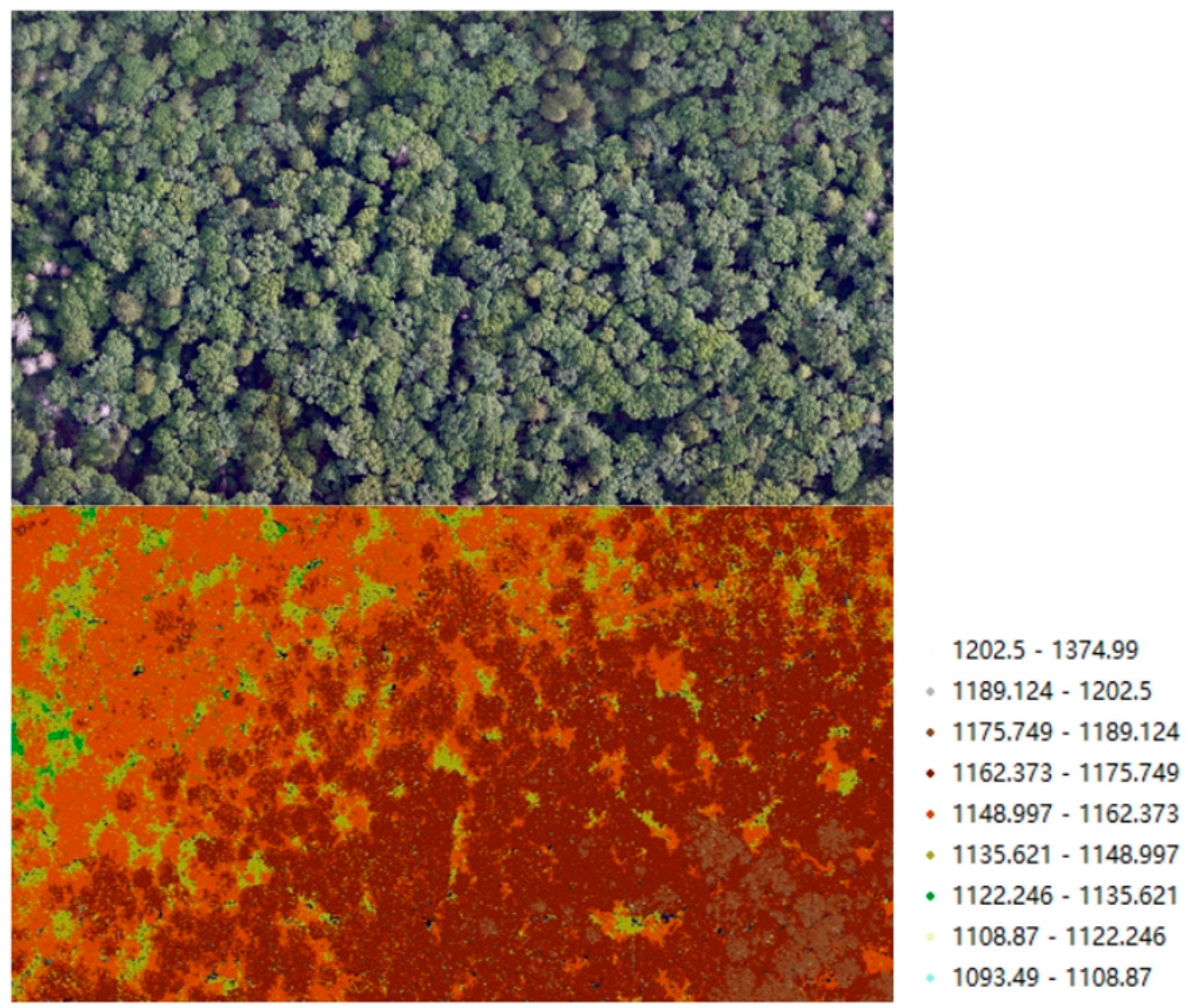
2.1. Study Area

The research was conducted in the Changbai Mountain National Nature Reserve, located in Jilin Province, China. This area features a varied terrain of mountains and hills and is influenced by a temperate continental monsoon climate. The elevation in this region varies between 700 and 1000 m above sea level, with an average yearly temperature of 5.14 °C and mean annual precipitation totaling 636.14 mm. The dominant vegetation in this region consists of natural deciduous broadleaf forests and mixed forests of broadleaf and conifer species. The broadleaf species include Betula ermanii (Erman’s birch), Quercus mongolica (Mongolian oak), and Acer pseudosieboldianum (Manchurian maple). Conifer species include Pinus koraiensis (Korean pine) and Abies nephrolepis (Korean fir). These species are of particular interest in this study, as their canopy heights are estimated to understand forest structure and dynamics in the reserve.

The broader study area used for GEDI-based canopy height estimation was defined according to the Boundary Coordinates Table for the Changbai Mountain National Nature Reserve in Jilin Province, issued by the Changbai Mountain Protection and Development Zone Management Committee in 2023. The reserve covers approximately 196,618 hectares and is located between 127°28′ E and 128°16′ E longitude and 41°42′ N to 42°25′ N latitude. Figure 1 illustrates the precise location of the study area.

2.2. Data Acquisition and Preprocessing

2.2.1. Airborne LiDAR Data

ALS data acquisition was conducted in June 2021 using a Bell helicopter equipped with a Galaxy Prime LiDAR scanner (Teledyne Optech, Vaughan, ON, Canada) and a 100-megapixel Phase One aerial camera (Phase One A/S, Copenhagen, Denmark). The operation was performed under optimal weather conditions, including clear skies, ample sunlight, and no wind, ensuring high-quality aerial imaging. The helicopter maintained a consistent flight altitude of 500 m, with a side overlap of approximately 45% and a flight line overlap of about 65%, providing thorough coverage. The LiDAR scanner operated with a laser wavelength of 1064 nm, a scanning angle ranging from 10° to 60°, and a pulse frequency of 50–100 kHz. This setup achieved an average point cloud density of 160 points per square meter. Additionally, aerial imagery in the red, green, and blue (RGB) bands was captured at a spatial resolution of 0.03 m, further enhancing the dataset quality [35].

Figure 2 illustrates a schematic diagram of the airborne LiDAR point cloud data acquired from the study area.

Furthermore, we selected 20 local sample locations at random and documented their geographic coordinates along with measurements of canopy and ground elevation. These positional data were then aligned with the corresponding airborne dataset to assess measurement consistency. As illustrated in the figure, both canopy and ground height values derived from the airborne sources demonstrated correlation coefficients exceeding 0.9, reflecting a strong level of agreement. Figure 3 illustrates that the airborne dataset is highly precise and well-suited for verifying forest height estimations.

2.2.2. GEDI V002 Data

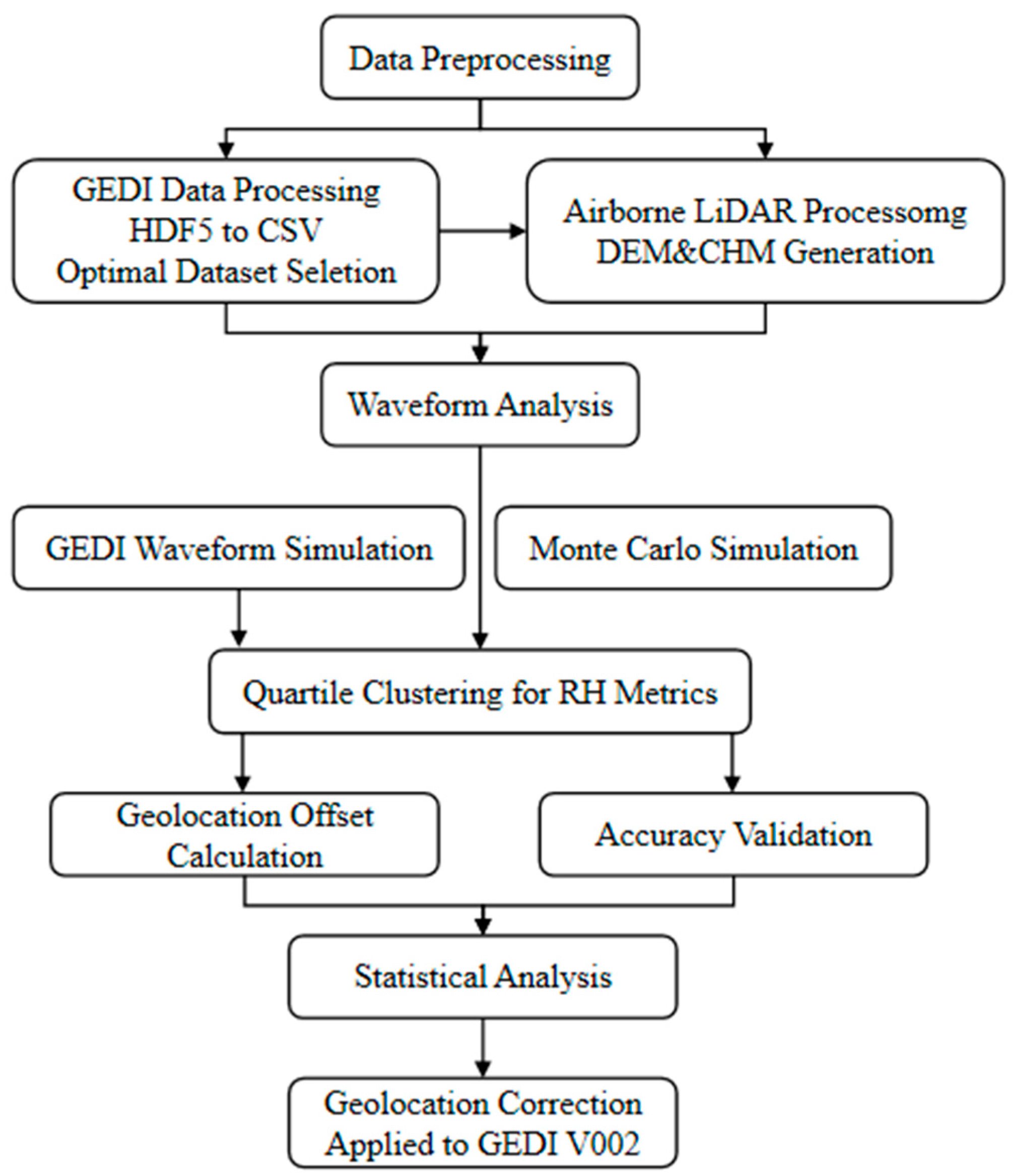
GEDI features the world’s first multi-beam, linear-mode LiDAR instrument, specifically engineered for high-resolution assessments of forest vertical structure. This cutting-edge technology is mainly employed to obtain accurate measurements of canopy height, vertical structure profiles, and ground elevation in temperate and tropical forest ecosystems. Detailed specifications of the instrument are provided in

Table 1. Main parameters description of GEDI.

Operational Characteristics	Operating Altitude	≈400 km
	Coverage Range	51.6° S to 51.6° N
	Reference System	WGS84
Beam and Measurement Details	Beam Diameter	≈25 m
	Along-Track Distance Between Footprints	60 m
	Across-Track Distance Between Footprints	600 m
	Number of Tracks	8 beam tracks
Laser Specifications	Laser Wavelength	1064 nm
	Pulse Width	14 ns
	Pulse Intensity	10 mJ
	Emission Frequency	242 Hz
Scanning Area	Scan Width	4.2 km

.

Compared to the ~70 m footprint size of ICESat/GLAS, GEDI offers a higher footprint density and demonstrates better performance when integrated with other data sources, such as Landsat and TANDEM-X, making it more suitable for observing forest structures and sub-canopy terrain. Data collection began on 25 March 2019, with the V2 version released on 16 April 2021 [36,37]. The Level 2A product delivers height metrics for individual footprints, such as ground elevation, canopy height, and relative height indices extracted from the waveform. Typically, GEDI observations achieve a high canopy penetration rate (>90%) [38]. However, when beam sensitivity exceeds 0.9—implying that canopy occupies less than 90% of the footprint—the reliability of the retrieved height may decrease.

GEDI data are organized into four distinct levels, reflecting the progressive stages of data processing. Level 1 encompasses geolocated waveform data, while Level 2 delivers footprint-specific canopy height measurements and profile metrics. Level 3 provides gridded data representing canopy height and its variations across spatial scales. Finally, Levels 4A and 4B focus on estimating aboveground carbon stocks, with Level 4A targeting footprint-level estimates and Level 4B offering gridded carbon stock data.

This study employed GEDI L1B and L2A products from the second version, which was released in 2021. In comparison to Version 1, GEDI Version 2 demonstrates significantly improved geolocation accuracy, with an average positional uncertainty of around 12 m. Furthermore, Version 2 incorporates the new parameter “selected_mode_flag,” designed to determine the most appropriate settings group (SG) for specific conditions. A total of 607 footprint data points were obtained within the study area and used for subsequent canopy height evaluation and analysis.

The GEDI Level 1B product (GEDI01_B) delivers geolocated waveform data, including corrected geolocations, smoothed waveforms, geophysical adjustments, and geolocation parameters for each laser shot across all eight GEDI beams. This dataset is derived by geolocating the raw waveform data from GEDI01_A. Delivered in HDF5 format, GEDI01_B features an average spatial resolution of 25 m per footprint. The product includes data for 85 beams, each containing detailed geolocation corrections, smoothed waveform parameters, and auxiliary information related to geolocation and geophysical adjustments.

The GEDI L2A product, generated through advanced algorithms, serves as a key dataset for deriving ground elevation and canopy height, making it essential for estimating forest canopy height. Unlike earlier versions, the L2A dataset undergoes more rigorous preprocessing and refined parameter adjustments, enabling higher accuracy in representing both ground elevation and canopy height. Additionally, the data integrates sophisticated modeling and specialized processing of terrain features, vegetation cover, and canopy structures, making it highly precise and well-suited for applications in forest research.

2.3. Method

This study investigates the impact of geolocation uncertainty in GEDI V002 data on the accuracy and reliability of forest canopy height estimation. Airborne laser scanning (ALS) and GEDI data were collected in 2020 and 2021, covering over 2000 hectares of forest within the Changbai Mountain National Nature Reserve. The analysis began with preprocessing GEDI and ALS data. GEDI simulation was employed to generate synthetic GEDI waveforms from ALS data based on GEDI footprint locations, which were then used to derive relative height metrics. A quartile clustering analysis was performed on these metrics to identify the most accurate relative height indicator for canopy height inversion.

To assess geolocation uncertainty, Monte Carlo simulations were applied to the ALS data by systematically displacing the center of each GEDI footprint. Randomly generated positional errors, based on GEDI geolocation uncertainty, were introduced into the analysis. For each GEDI footprint within the validation region, height errors were computed by comparing the original footprint with 300 simulated GEDI footprint locations. The simulated point yielding the highest extraction accuracy was identified for each footprint, and the average positional offset across all footprints in the study area was calculated. This resulted in a mean geolocation offset of 8.4 m, with a directional shift of 14.3° southwest relative to the original GEDI coordinates. This average offset was then applied as a uniform correction to the GEDI V002 footprint locations. Finally, canopy height estimates before and after geolocation correction were compared, and accuracy validation analyses were conducted to assess the effectiveness of the correction method. The complete methodological workflow is illustrated in Figure 4 [39].

After applying the estimated geolocation correction, all subsequent analyses—including canopy height estimation and accuracy validation—were based on the original GEDI V002 data. This ensured that GEDI data were consistently used for both geolocation correction and canopy height analysis, with ALS-derived waveforms serving only as spatial references.

Monte Carlo simulations were used to model geolocation uncertainty by randomly displacing each GEDI footprint up to 300 times based on known error distributions. Height errors were computed across these simulations to identify the displacement with the highest agreement with ALS-derived metrics, which was then applied as the correction offset. The effectiveness of this correction was assessed by comparing canopy height estimates before and after adjustment. A full overview of the methodological workflow is presented in Figure 4.

To ensure the robustness and generalizability of the model, a 5-fold random cross-validation was conducted on the dataset. The data were randomly divided into five subsets of equal size. In each iteration, four subsets were used to train the model, and the remaining subset was used for validation. This process was repeated five times, and the average accuracy metrics (RMSE and ME) were calculated. This strategy minimizes the risk of overfitting and provides a more reliable estimate of model performance.

2.3.1. Data Preprocessing

(1)

ALS Data

The 2020 airborne LiDAR point cloud data from the Changbai Mountain region were used to produce a high-precision DEM for the Changbai Mountain National Nature Reserve. Following the denoising process, an enhanced progressive densification triangulated irregular network (TIN) filtering algorithm was employed to classify ground points effectively. The DEM was then generated using an inverse distance weighting (IDW) interpolation algorithm, with a spatial resolution of 1 m. Slope analysis was conducted on the DEM data, and a terrain slope map of the forest area in Changbai Mountain was produced based on the 1 m resolution elevation product. This raster-based analytical process is consistent with previous studies involving GIS and remote sensing techniques for forest landscape evaluation [40].

(2)

GEDI Data

To integrate GEDI data with the validation dataset, the downloaded GEDI L2A data were first spatially clipped to the extent of the ALS data and converted to a compatible format. Subsequently, only footprint points with a “quality_flag” value of 1 were retained as valid footprints, while all other points were discarded [41]. Since the coordinates of GEDI data use the WGS84 geographic coordinate system, the coordinate system was converted to the corresponding UTM projection system used by the LiDAR data to ensure positional alignment.

2.3.2. Algorithm Selection for GEDI Data

GEDI L2A generates waveform processing results using six different algorithm configurations, each employing various smoothing parameters, waveform start thresholds, and waveform end thresholds. These algorithms are designed to extract key information, such as surface elevation and vegetation height, from the GEDI data. The six algorithms used in this study are “AmpSim”, “AmpSDE”, “WavHgt”, “RH”, “AnomHeight”, and “Stat”, each with distinct processing approaches:

(1)

AmpSim: This algorithm simulates the waveform amplitude using a simple sine wave model, primarily focused on generating a synthetic representation of the waveform.

(2)

AmpSDE: Similar to AmpSim, but with an additional smoothing operation applied to the waveform for better fitting to surface features, particularly in dense vegetation areas.

(3)

WavHgt: This algorithm estimates the surface height by analyzing the peak of the waveform and adjusting for vegetation interference, making it useful for areas with complex canopy structures.

(4)

RH: The Relative Height algorithm extracts vegetation height by calculating the difference between the ground surface and canopy return points, making it particularly effective for canopy height estimation.

(5)

AnomHeight: This algorithm focuses on identifying anomalous waveform behaviors, particularly in areas with mixed vegetation types or significant topographic variations. It provides a robust measure of canopy height with high sensitivity.

(6)

Stat: A statistical approach that processes waveforms based on predefined statistical models, aiming for broad applicability across diverse environments and vegetation types.

Each algorithm offers a different processing strategy, with default optimal results for each beam available in the root directory. However, alternative configurations for certain algorithms have been found to yield more accurate estimates of surface elevation and forest canopy height under specific conditions.

In this study, the “sensitivity” parameter was employed to evaluate the performance of each algorithm. Sensitivity was assessed by calculating the median, standard deviation, and other metrics across all six algorithm configurations. The results of this evaluation are presented in

Table 2. Quality evaluation of six algorithm configurations.

	Median	Var	Std
Algorithm 1	0.54	1040.20	32.25
Algorithm 2	0.85	208.34	14.43
Algorithm 3	0.64	736.6	27.14
Algorithm 4	0.54	1040.2	32.25
Algorithm 5	0.91	100.63	10.03
Algorithm 6	0.77	339.95	18.44

.

Among the six algorithms, “AnomHeight” (Algorithm 5) exhibits a median value of 0.91, significantly outperforming the others. In comparison, “AmpSim” (Algorithm 1) and “RH” (Algorithm 4) have medians of 0.54, “AmpSDE” (Algorithm 2) has 0.85, “WavHgt” (Algorithm 3) has 0.64, and “Stat” (Algorithm 6) has 0.77. This indicates that “AnomHeight” demonstrates higher overall sensitivity, better reflecting variations in the target metrics. Furthermore, the combination of the median and standard deviation for “AnomHeight” suggests that it consistently delivers stable and efficient sensitivity results under most conditions. As a result, “AnomHeight” not only outperforms the other algorithms in overall performance but also shows greater advantages in terms of sample robustness and reproducibility across various scenarios. Therefore, “AnomHeight” was selected for subsequent analyses.

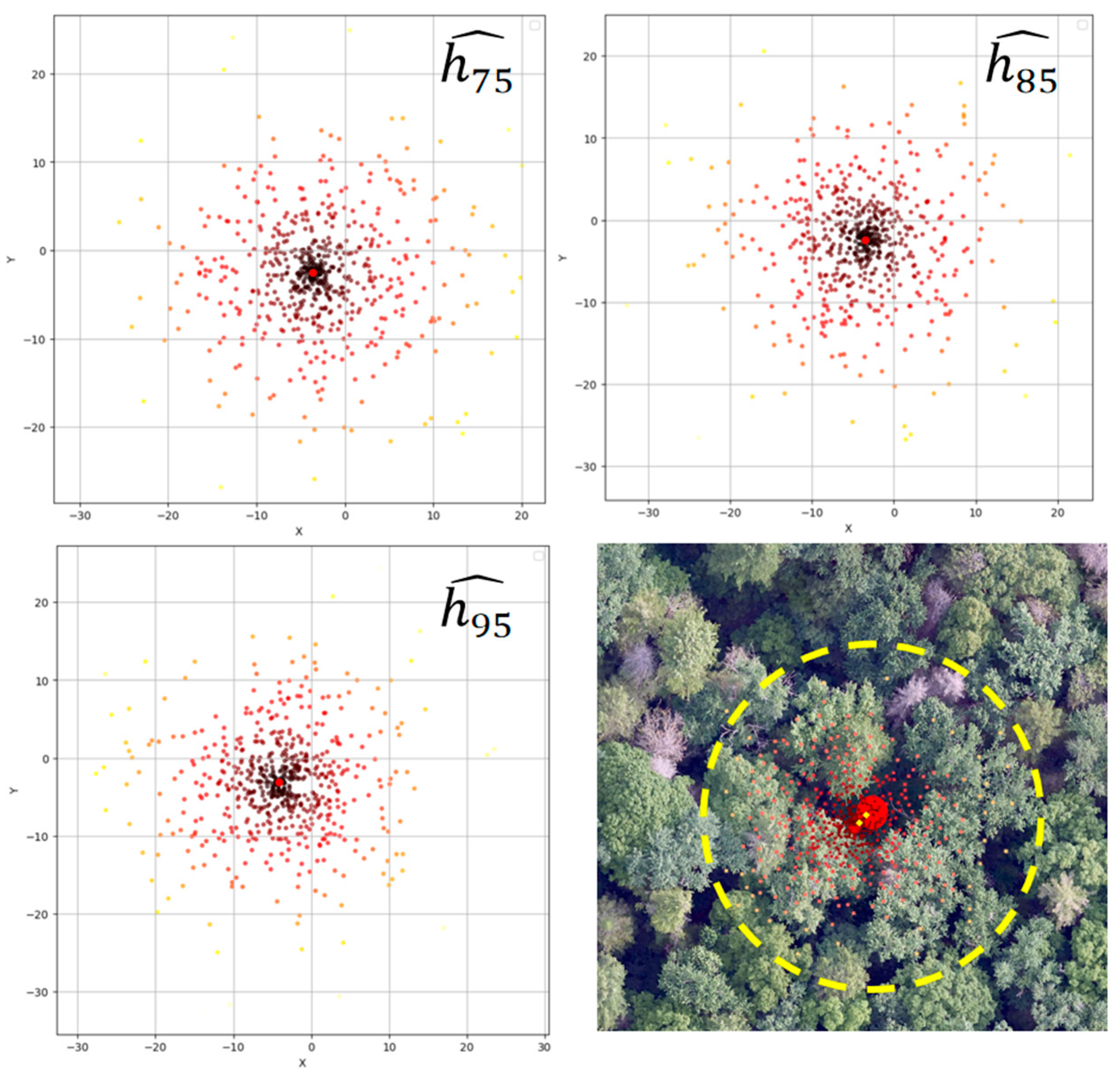
2.3.3. Monte Carlo Simulation

The fundamental concept behind the Monte Carlo method involves estimating a desired statistic or expected value by generating numerous random samples and computing outcomes derived from these samples [42]. This method is particularly suitable for problems that cannot be solved using traditional analytical methods, especially complex or probabilistic problems that are difficult to resolve directly. A key feature of the Monte Carlo method is its reliance on a large number of independent trials for approximate computation.

In this study, we applied the Monte Carlo simulation approach to adjust the reported footprint positions from the GEDI product. Each footprint location was shifted by a randomly generated positional error modeled based on GEDI geolocation uncertainty. The adjustment was calculated using the following formula:

$$x_i^{\mathrm{*}}=x+s_i\cos \left({\theta }_i\right)$$

(1)

$$y_i^{*}=y+s_i\mathit{sin}\left({\theta }_i\right)$$

(2)

In the formula, $\left(x_i^{*},y_i^{*}\right)$ represents the coordinates of the displaced GEDI footprint center, $\left(x,y\right)$ represents the original GEDI footprint center coordinates, $s_i$ is a randomly sampled number that follows a normal distribution, simulating GEDI geolocation uncertainty $~\mathrm{N}\left(\mu =0 \mathrm{m},\sigma =10 \mathrm{m}\right), {\theta }_i$ is a random angle sampled from a uniform distribution constrained within$0°\le {\theta }_i<360°$, and n represents the number of random samples. We set n = 300 to ensure more reliable simulation results [43]. Furthermore, setting n = 300 allows for the random simulation of displaced center coordinates in all directions around the original GEDI footprint center. As shown in Figure 5, the red circles represent the coverage of GEDI footprints within the study area, while the black circles depict the coverage of 300 displaced footprints.

The majority of the displaced footprints are clustered around the original GEDI footprint locations; however, some have centers positioned approximately 12 m away from the GEDI footprint (Figure 5b). The geolocation uncertainty of GEDI~N $\left(\mu =0 \mathrm{m},\sigma =10 \mathrm{m}\right)$implies that 95% of GEDI footprint locations fall within a 20 m radius. This indicates that GEDI geolocation uncertainty can sometimes lead to GEDI data capturing portions of forest canopy that are adjacent to, but spatially non-overlapping with, the footprint location reported by the GEDI product.

ALS data were collected for both the footprint locations specified by the GEDI product (marked by red circle in Figure 5a) and the 300 simulated GEDI footprints (shown as black circles in Figure 5b). These data were then utilized to generate GEDI waveforms for each footprint. On average, each footprint contained 2894 ALS returns, which were used to simulate the corresponding GEDI waveforms. The GEDI Simulator, as developed by Hancock [33], was utilized for this simulation process. Figure 6 illustrates an example of the GEDI data simulated from ALS data. The relative height metrics derived from these simulations are denoted as $\widehat{h_p}$.

In this research, the relative height values $\widehat{h_{95}}, \widehat{h_{85}}, \mathrm{a}\mathrm{n}\mathrm{d} \widehat{h_{75}}$ were selected based on their common use in remote sensing studies as key indicators for canopy structure. These values represent different percentiles of the canopy height distribution and are commonly used to capture variations in canopy density and surface structure [44]. Specifically, $\widehat{h_{95}}$ corresponds to the 95th percentile, often used to estimate the upper canopy or top of the canopy; $\widehat{h_{85}}$ and $\widehat{h_{75}}$ are typically used to assess lower canopy heights or vegetation structure within the canopy. These relative height values are well-established in the literature and have been shown to be effective in characterizing forest canopy height and structure, which is why they were chosen for the simulation in this study [38]. To derive these simulated relative heights, three distinct ground-fitting algorithms were applied. Although the simulation process can account for GEDI noise, it necessitates site-specific parameters, such as beam sensitivity, which is influenced by the canopy structure at the given location.

Building on the approach utilized in prior research, which simulated GEDI waveforms from ALS data for forest assessments [38], this study employed a noiseless, Gaussian-based ground-fitting simulation to derive the relative height metrics $\widehat{h_p}$.

To evaluate the accuracy of these simulated values, we compared them with ALS-derived reference heights. The results showed that the simulated relative heights had an average bias of less than 0.22 m and a root mean square error (RMSE) of under 5.7 m, indicating high reliability for subsequent analysis [33]. Considering the canopy heights observed in the forest under study, the bias was deemed insignificant. The RMSE, which reflects random variation, suggests that the simulated values might either overestimate or underestimate the true canopy heights.

To evaluate the impact of GEDI geolocation uncertainty on forest canopy height inversion, a comparison was conducted between the simulated relative heights obtained from ALS data at the original GEDI footprint locations (denoted as $\widehat{h_p}\left(x,y\right)$) and those calculated from the displaced footprint positions ($\widehat{h_p}\left(x_i^{\mathrm{*}},y_i^{\mathrm{*}}\right)$, where $i=\mathrm{1,2},3\dots 100$). The variability among the 300 simulated values of $\widehat{h_p}\left(x_i^{\mathrm{*}},y_i^{\mathrm{*}}\right)$ was quantified using the 50th percentile (i.e., the median), as well as the 25th and 75th percentiles. Additionally, the interquartile range (IQR), defined as the difference between the 75th and 25th percentiles, was calculated to further assess the spread of the data. Non-parametric statistical methods were employed because, for each GEDI footprint within the study area, 300 simulated values were generated to reflect potential geolocation offsets and these values did not follow a normal distribution. This outcome is consistent with the findings, as the modeled geolocation errors followed a normal distribution, but the vegetation structure around most footprint positions in this study was heterogeneous.

After generating 300 simulated positions for each GEDI footprint and computing the corresponding canopy height errors, the displacement that yielded the minimum error was recorded. By analyzing the optimal displacement vectors across all footprints in the validation region, we determined a consistent geolocation offset. The mean magnitude of this offset was 8.4 m, and its average direction was 14.3° toward the southwest (i.e., approximately toward 194.3° azimuth). This empirical result was used to apply a uniform correction to all GEDI footprints in the region.

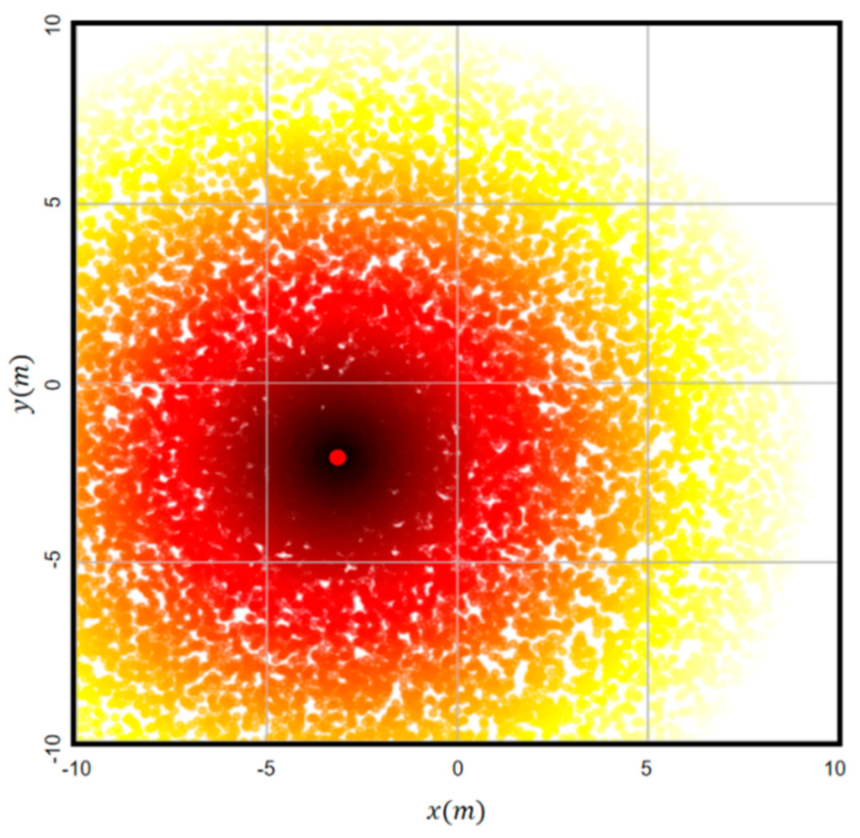
2.3.4. GEDI Geolocation Offset

The GEDI geolocation offset paired-search method is an algorithm based on precise matching and pairwise comparison, designed to identify spatial deviations in GEDI data coordinates [45]. This method identifies and quantifies spatial shifts caused by positioning errors or satellite orbital changes by iteratively matching the actual location of each measurement point with its theoretical location (or reference geographic information). Specifically, reference data or ground observation points are first selected as a baseline. Each GEDI measurement point is then compared with the reference points to calculate spatial discrepancies. These discrepancies are used to quantify the geolocation offset and subsequently apply corrections. This method effectively detects and rectifies geolocation errors in GEDI data, providing more accurate data support for high-precision geospatial analyses.

For each GEDI footprint point in the validation region, comparisons were made with the 300 simulated GEDI footprint points, and height value$\widehat{h_{95}}, \widehat{h_{85}}$, and $\widehat{h_{75}}$ errors were extracted. The simulated point with the highest extraction accuracy for each footprint was identified. Figure 7 illustrates the process of one-to-one matching for each footprint and its corresponding simulated points to locate the optimal position, using a single GEDI footprint as an example.

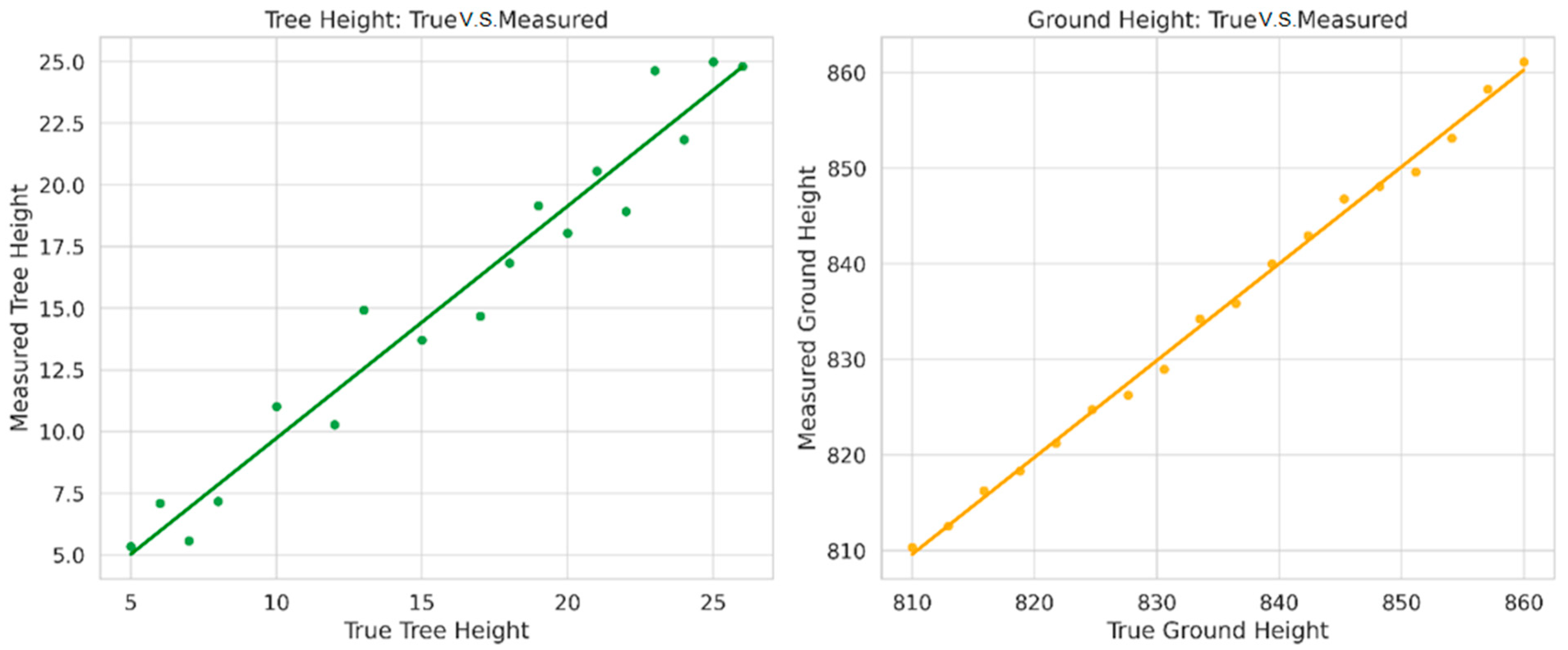
2.3.5. Accuracy Validation

To assess the difference between the predicted and reference canopy heights, we used the root mean square error (RMSE) as the main metric for evaluating accuracy. In this study, predicted heights refer to the canopy height estimates derived from GEDI-simulated waveform metrics using a sensitivity-based model selection approach. Reference heights represent true canopy height values directly calculated from high-resolution ALS (airborne LiDAR scanning) data within each GEDI footprint. Additionally, the mean error (ME) was computed to evaluate potential systematic bias in the predictions [46,47]:

$$\mathrm{R}\mathrm{M}\mathrm{S}\mathrm{E}=\sqrt{{\displaystyle \frac{1}{\mathrm{N}}}\sum _{\mathrm{i}=1}^{\mathrm{N}}{\left({\widehat{\mathrm{y}}}_{\mathrm{i}}-{\mathrm{y}}_{\mathrm{i}}\right)}^2}$$

(3)

$$\mathrm{M}\mathrm{E}={\displaystyle \frac{1}{\mathrm{N}}}\sum _{\mathrm{i}=1}^{\mathrm{N}}\left({\widehat{\mathrm{y}}}_{\mathrm{i}}-{\mathrm{y}}_{\mathrm{i}}\right)$$

(4)

In this context, ${\widehat{\mathrm{y}}}_{\mathrm{i}}$ refers to the predicted value from the model, while ${\mathrm{y}}_{\mathrm{i}}$ denotes the reference value at sample i. Based on this definition, a positive mean error (ME) indicates that the model’s predictions generally exceed the true values in comparison to the reference data.

The mean relative error (MRE) was calculated as follows:

$$MRE={\displaystyle \frac{1}{n}}\sum _{i=1}^n\left|{\displaystyle \frac{H_{GEDI,i}-H_{ALS,i}}{H_{ALS,i}}}\right|$$

(5)

where $H_{GEDI,i}$ is the estimated canopy height from GEDI at footprint i and $H_{ALS,i}$ is the corresponding reference height from ALS data.

3. Results

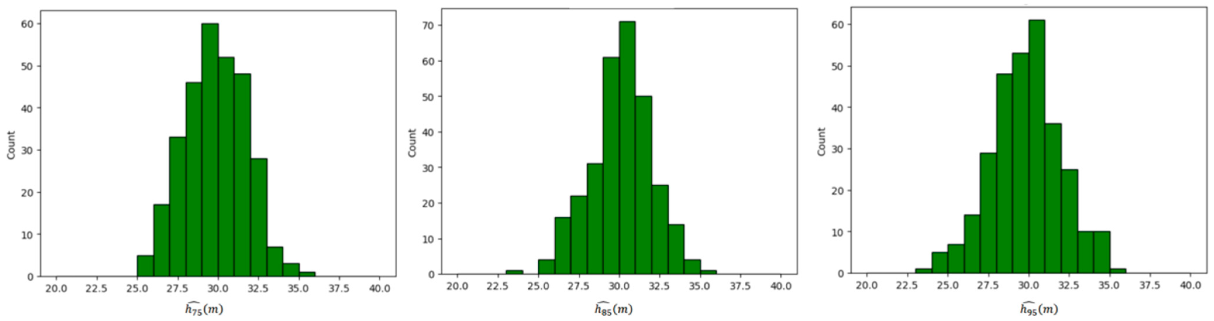
3.1. The Influence of GEDI Geolocation Uncertainty on Forest Canopy Height Estimation

Figure 8 illustrates the impact of GEDI geolocation uncertainty on forest canopy height estimation, focusing on a representative footprint located in the northern part of the study area (highlighted in Figure 5a). The three relative height values derived from ALS data at GEDI-indicated footprint positions are 28.78 m, 30.62 m, and 31.46 m, indicating minimal intra-footprint variability and a canopy structure dominated by tall, consistent vegetation.

A 5-fold cross-validation yielded an RMSE of 3.6 m and ME of −0.3 m, indicating a slight underestimation bias compared to the ALS reference data. The histogram in Figure 8 shows the distribution of 300 simulated relative height values (green bars), generated by displacing the GEDI footprint using a Monte Carlo-based method. If canopy structure were homogeneous across all displacement positions, the histogram would exhibit a narrow peak. However, observed differences (maximum spread of 12.24 m, 12.67 m, and 13.35 m for the three relative height metrics) suggest considerable variability in canopy conditions across the simulated footprint range.

The values simulated—$\widehat{h_{95}}, \widehat{h_{85}}$, and $\widehat{h_{75}}$—correspond to 95%, 85%, and 75% cumulative energy returns and reflect canopy height relative to ground elevation. Even slight changes in footprint position capturing tall trees or gaps may influence these percentile-based height metrics. The simulation reveals that a geolocation-induced variability of approximately 2 m in relative height is present at the 50% level. Given an average canopy height of around 30 m, this represents a moderate but non-negligible level of uncertainty in GEDI canopy height retrieval.

To further quantify these uncertainties, Figure 9 presents the interquartile range (IQR) of the three simulated metrics at 300 offset positions per GEDI footprint, for a total of 445 footprints across both forested and non-forested regions. The IQR for $\widehat{h_{75}}$ ranges from 1.68 m to 18.19 m and for $\widehat{h_{95}}$ from 16.05 m to 24.35 m. Simulated height ranges are broader in regions with greater canopy complexity or variable terrain.

Interestingly, the IQR values display weak correlations with the actual canopy height: 0.31 for $\widehat{h_{75}}$, 0.32 for $\widehat{h_{85}}$, and 0.17 for $\widehat{h_{95}}$. These low coefficients suggest that height variation due to geolocation offset is not linearly dependent on canopy height. Rather, it indicates that the positional uncertainty causes spatial sampling of heterogeneity that is independent of the vertical structure magnitude.

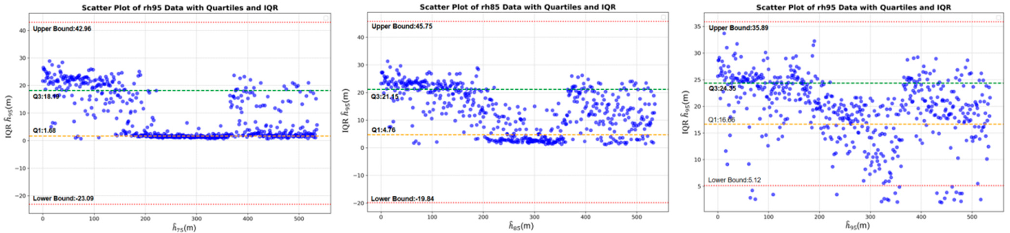
3.2. Impact of GEDI Geolocation Offset on Forest Height Extraction

To better understand the positional sensitivity, a Monte Carlo simulation was conducted to derive optimal footprint positions for each GEDI location, based on best-matching $\widehat{h_{95}}, \widehat{h_{85}}$, and $\widehat{h_{75}}$ values against ALS reference data. Figure 10 shows correlation coefficient plots comparing these simulated values with their counterparts at GEDI-reported footprint positions.

In the figure, three different colors are used to distinguish points based on their position relative to the regression line: Green points represent data above the regression line with a significantly larger increase (greater than 1.25 times the regression line). These points indicate actual values that are substantially higher than the model predictions. Red points represent data below the regression line with a significantly lower increase (less than 0.75 times the regression line). These points indicate actual values that are substantially lower than the model predictions. Black points represent data near the regression line, within the range of 0.75 to 1.25 times. These points indicate actual values that are generally consistent with the model predictions.

The correlation coefficients for the simulated $\widehat{h_{95}}, \widehat{h_{85}}$, and $\widehat{h_{75}}$ are 0.62, 0.59, and 0.49, respectively, indicating that the simulation performs best for $\widehat{h_{95}}$.

The results presented in Figure 11 illustrate the geolocation offsets of GEDI data calculated through point-by-point geolocation matching based on $\widehat{h_{95}}$-simulated canopy height data. The optimal position with the highest recorded accuracy for each point was identified to determine the geolocation offsets of the GEDI data. The study found that the average geolocation offset for points in the study area was 8.4 m, with a directional shift of 14.3° southwest of the central coordinate.

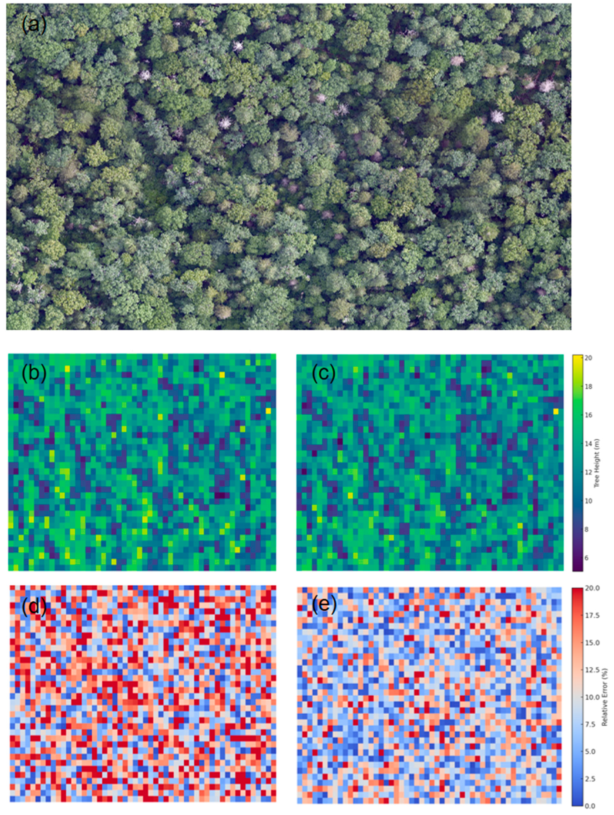
3.3. GEDI Forest Height Inversion

The results from Experiment 4.2 indicate that the overall geolocation offset for GEDI data in the study area is x: −8.14 and y: −2.07. Based on these findings, the GEDI data for the study area were geolocation-corrected, and a new forest canopy height map was generated. This corrected map was compared with the original, uncorrected map. The experimental results are presented in Figure 12.

As shown in Figure 12, this set of images provides a comprehensive visualization and validation of the forest canopy height inversion and the effectiveness of the geolocation correction process. Figure 12a displays the high-resolution airborne remote sensing imagery of the study area within the Changbai Mountain National Nature Reserve. The dense and complex canopy structure is clearly visible, providing a visual reference for the subsequent inversion and accuracy analysis.

Figure 12b presents the initial canopy height map obtained by inverting GEDI V002 data without any geolocation correction. The spatial distribution of canopy height appears reasonable overall, but noticeable discrepancies and local inconsistencies are evident when compared to the reference imagery, likely attributable to geolocation offsets between GEDI footprints and the actual ground features.

Following the application of the Monte Carlo-based geolocation correction method, the updated canopy height inversion map is shown in Figure 12c. Compared to Figure 12b, the corrected map exhibits a smoother and more continuous spatial pattern of canopy height. The inversion results align more closely with the observed structure of the forest canopy from the airborne imagery, suggesting that the correction procedure effectively mitigates positional biases introduced by geolocation uncertainties.

Figure 12d,e further quantify these improvements through accuracy validation analyses. In Figure 12d, the relative errors between the airborne LiDAR-derived canopy heights (reference data) and the uncorrected GEDI-derived canopy heights (test data) are visualized. Prior to correction, the spatial distribution of errors is highly heterogeneous, with numerous regions exhibiting significant deviations. The calculated mean relative error before correction was 11.92%, indicating a considerable impact of geolocation uncertainty on the reliability of the inversion results.

In contrast, Figure 12e illustrates the relative error distribution after the geolocation correction was applied. Compared to the uncorrected case, the spatial pattern of errors is more uniform, and the magnitude of errors is notably reduced. The mean relative error decreased substantially to 8.55%, demonstrating a clear enhancement in canopy height estimation accuracy. The reduction in error highlights the effectiveness of the proposed method in compensating for GEDI footprint geolocation inaccuracies, ultimately improving the precision and reliability of forest structure assessments derived from GEDI data.

Overall, the results visualized in Figure 12 confirm that correcting for geolocation uncertainty is crucial for accurate canopy height retrieval from spaceborne LiDAR data. The methodological framework implemented in this study—combining Monte Carlo simulations with positional offset correction—proves to be an effective strategy for addressing this challenge and enhancing the quality of GEDI-based forest measurements. These improvements are critical for subsequent ecological analyses and applications relying on accurate forest canopy structure information.

4. Discussion

In recent years, increasing attention has been devoted to the assessment and mitigation of uncertainties in spaceborne LiDAR systems, particularly in the GEDI mission. Among the various sources of error, geolocation inaccuracies are recognized as a critical factor affecting the reliability of canopy height retrievals. This study contributes to the growing body of literature by quantifying the impact of GEDI geolocation uncertainty in a densely forested area and validating a Monte Carlo-based correction method using high-resolution ALS data.

Our findings reveal a consistent geolocation offset in the GEDI L2A data, with an average displacement of 8.4 m oriented toward the southwest. This directional bias is in agreement with previous studies conducted in different ecosystems, such as Liu et al. (2022) [48] and Lang et al. (2022) [49], suggesting a systematic trend rather than random geolocation error. While these prior investigations focused on tropical or mixed forest environments, our results extend these observations to temperate broadleaf–coniferous forests, indicating that such biases are prevalent across diverse forest types.

By introducing simulated footprints offset from the GEDI center coordinates, we observed a canopy height variability of up to 13.35 m, with a median deviation of approximately 2.02 m. Although this deviation constitutes a relatively small fraction (~6.7%) of the average canopy height in our study area, it has non-negligible implications for forest structure modeling, biomass estimation, and carbon stock assessments. These findings are consistent with Xu et al. (2023) [50], who emphasized the role of sub-footprint variability in influencing GEDI waveform-derived metrics.

The Monte Carlo simulation approach employed in this study effectively reduced the mean relative error of GEDI-estimated canopy heights from 11.92% to 8.55%. Compared to more complex machine learning-based methods, such as convolutional neural networks (CNNs) or waveform deconvolution algorithms, our correction strategy is relatively simple and computationally efficient [51]. This makes it well-suited for large-scale applications, especially when computational resources are limited.

Despite the improvement achieved through geolocation correction, several limitations should be acknowledged. First, the ALS data used for GEDI simulation were acquired on a single date and may not fully capture temporal variations in forest structure, especially considering phenological or disturbance-induced changes. Second, our method assumes a uniform probability distribution of GEDI footprint offsets within the circular buffer, which may not precisely reflect the real-world geolocation error distribution. Third, the GEDI waveform simulation process does not account for atmospheric effects or beam divergence, which could further influence the waveform shape and height metrics.

We further examined the interquartile range (IQR) of simulated canopy heights and found a weak correlation with actual canopy height (Pearson’s r = 0.17–0.32 across forest types). This suggests that factors such as topographic complexity, canopy structure heterogeneity, and edge effects—not height alone—contribute significantly to displacement-induced uncertainty. Future correction strategies should consider incorporating high-resolution ancillary data to better represent such fine-scale spatial variation.

This study also faces limitations in temporal validation. Our analysis relied on ALS and GEDI data from specific years (2020 and 2021), which may not adequately account for temporal variations due to seasonal growth dynamics or disturbance events. We have acknowledged this constraint in the revised discussion and propose the use of multi-temporal ALS or UAV-LiDAR datasets in future work to assess model stability across time. Additionally, fusing GEDI data with optical remote sensing products from Sentinel-2 or Landsat-9 could improve the spatiotemporal characterization of canopy variability.

In summary, this study highlights that moderate geolocation offsets can result in non-negligible errors in canopy height estimation. While our Monte Carlo-based correction method offers an accessible and effective solution, its global and long-term applicability requires further investigation. We believe our findings contribute meaningful insights into the operational challenges of using GEDI data for forest monitoring and carbon accounting, and we encourage continued efforts toward comprehensive validation across ecosystems and timescales.

5. Conclusions

This study investigates the impact of geolocation uncertainty on GEDI-derived canopy height estimates in the Changbai Mountain National Nature Reserve. The results show that the average geolocation offset in GEDI L2A data is 8.4 m, with a consistent southwestward directional bias. By applying a Monte Carlo-based correction approach, we reduced the mean relative error in canopy height estimates from 11.92% to 8.55%. The variability observed in simulated canopy heights, up to 13.35 m, highlights the significant role of footprint displacement in height estimation, particularly in structurally heterogeneous landscapes.

This research provides a straightforward and computationally efficient method for geolocation correction, making it suitable for large-scale applications. Furthermore, our findings underline the importance of considering footprint-level structure in GEDI-based forest assessments and contribute to enhancing the reliability of GEDI data in complex forest environments. These results offer valuable insights for future forest structure and ecosystem service assessments, as well as improvements in GEDI’s global canopy height estimation.

References

1. Li, C.; Wu, J.; Zhang, F.; Huang, X. Forest Carbon Sinks in Chinese Provinces and Their Impact on Sustainable Development Goals. Forests 2025, 16, 83. [Google Scholar] [CrossRef]
2. Wang, J.; Zhang, M.; Zhou, S.; Huang, Y. Research on the Spatiotemporal Evolution and Driving Factors of Forest Carbon Sink Increment—Based on Data Envelopment Analysis and Production Theoretical Decomposition Model. Forests 2025, 16, 104. [Google Scholar] [CrossRef]
3. Li, Y.; Dan, L.; Peng, J.; Yang, Q.; Yang, F. Increase in the variability of terrestrial carbon uptake in response to enhanced future ENSO modulation. Atmos. Ocean. Sci. Lett. 2025, 18, 100508. [Google Scholar] [CrossRef]
4. Bustamante, M.M.; Roitman, I.; Aide, T.M.; Alencar, A.; Anderson, L.O.; Aragao, L.; Asner, G.P.; Barlow, J.; Berenguer, E.; Chambers, J.; et al. Toward an integrated monitoring framework to assess the effects of tropical forest degradation and recovery on carbon stocks and biodiversity. Glob. Change Biol. 2016, 22, 92–109. [Google Scholar] [CrossRef] [PubMed]
5. Wang, Z.; Zhang, Y.; Li, F.; Gao, W.; Guo, F.; Li, Z.; Yang, Z. Regional mangrove vegetation carbon stocks predicted integrating UAV-LiDAR and satellite data. J. Environ. Manag. 2024, 368, 122101. [Google Scholar] [CrossRef] [PubMed]
6. Shugart, H.H.; Saatchi, S.; Hall, F.G. Importance of structure and its measurement in quantifying function of forest ecosystems. J. Geophys. Res. Biogeosci. 2010, 115, 1–16. [Google Scholar] [CrossRef]
7. LaRue, E.A.; Hardiman, B.S.; Elliott, J.M.; Fei, S. Structural diversity as a predictor of ecosystem function. Environ. Res. Lett. 2019, 14, 114011. [Google Scholar] [CrossRef]
8. Xi, Y.; Tian, Q.; Zhang, W.; Zhang, Z.; Tong, X.; Brandt, M.; Fensholt, R. Quantifying understory vegetation density using multi-temporal Sentinel-2 and GEDI LiDAR data. GISci. Remote Sens. 2022, 59, 2068–2083. [Google Scholar] [CrossRef]
9. Guo, Q.; Du, S.; Jiang, J.; Guo, W.; Zhao, H.; Yan, X.; Zhao, Y.; Xiao, W. Combining GEDI and sentinel data to estimate forest canopy mean height and aboveground biomass. Ecol. Inform. 2023, 78, 102348. [Google Scholar] [CrossRef]
10. Lang, N.; Jetz, W.; Schindler, K.; Wegner, J.D. A high-resolution canopy height model of the Earth. Nat. Ecol. Evol. 2023, 7, 1778–1789. [Google Scholar] [CrossRef]
11. Musthafa, M.; Singh, G.; Kumar, P. Comparison of forest stand height interpolation of GEDI and ICESat-2 LiDAR measurements over tropical and sub-tropical forests in India. Environ. Monit. Assess. 2022, 195, 71. [Google Scholar] [CrossRef] [PubMed]
12. Abdalati, W.; Zwally, H.J.; Bindschadler, R.; Csatho, B.; Farrell, S.L.; Fricker, H.A.; Harding, D.; Kwok, R.; Lefsky, M.; Markus, T.; et al. The ICESat-2 Laser Altimetry Mission. Proc. IEEE 2010, 98, 735–751. [Google Scholar] [CrossRef]
13. Neuenschwander, A.; Guenther, E.; White, J.C.; Duncanson, L.; Montesano, P. Validation of ICESat-2 terrain and canopy heights in boreal forests. Remote Sens. Environ. 2020, 251, 112110. [Google Scholar] [CrossRef]
14. Chen, L.; Ren, C.; Zhang, B.; Wang, Z.; Liu, M.; Man, W.; Liu, J. Improved estimation of forest stand volume by the integration of GEDI LiDAR data and multi-sensor imagery in the Changbai Mountains Mixed forests Ecoregion (CMMFE), northeast China. Int. J. Appl. Earth Obs. Geoinf. 2021, 100, 102326. [Google Scholar] [CrossRef]
15. Schwartz, M.; Ciais, P.; Ottlé, C.; De Truchis, A.; Vega, C.; Fayad, I.; Brandt, M.; Fensholt, R.; Baghdadi, N.; Morneau, F.; et al. High-resolution canopy height map in the Landes forest (France) based on GEDI, Sentinel-1, and Sentinel-2 data with a deep learning approach. Int. J. Appl. Earth Obs. Geoinf. 2024, 128, 103711. [Google Scholar] [CrossRef]
16. Qi, W.; Saarela, S.; Armston, J.; Ståhl, G.; Dubayah, R. Forest biomass estimation over three distinct forest types using TanDEM-X InSAR data and simulated GEDI lidar data. Remote Sens. Environ. 2019, 232, 111283. [Google Scholar] [CrossRef]
17. Zhu, X.; Nie, S.; Zhu, Y.; Chen, Y.; Yang, B.; Li, W. Evaluation and Comparison of ICESat-2 and GEDI Data for Terrain and Canopy Height Retrievals in Short-Stature Vegetation. Remote Sens. 2023, 15, 4969. [Google Scholar] [CrossRef]
18. Wang, C.; Jia, D.; Lei, S.; Numata, I.; Tian, L. Accuracy Assessment and Impact Factor Analysis of GEDI Leaf Area Index Product in Temperate Forest. Remote Sens. 2023, 15, 1535. [Google Scholar] [CrossRef]
19. Lahssini, K.; Baghdadi, N.; le Maire, G.; Fayad, I. Influence of GEDI Acquisition and Processing Parameters on Canopy Height Estimates over Tropical Forests. Remote Sens. 2022, 14, 6264. [Google Scholar] [CrossRef]
20. Rajab Pourrahmati, M.; le Maire, G.; Baghdadi, N.; Ferraco Scolforo, H.; Alcarde Alvares, C.; Stape, J.L.; Fayad, I. Effects of Eucalyptus plantation characteristics and environmental factors on GEDI waveform metrics. Int. J. Remote Sens. 2024, 45, 3737–3763. [Google Scholar] [CrossRef]
21. Marselis, S.M.; Keil, P.; Chase, J.M.; Dubayah, R. The use of GEDI canopy structure for explaining variation in tree species richness in natural forests. Environ. Res. Lett. 2022, 17, 045003. [Google Scholar] [CrossRef]
22. Tang, H.; Stoker, J.; Luthcke, S.; Armston, J.; Lee, K.; Blair, B.; Hofton, M. Evaluating and mitigating the impact of systematic geolocation error on canopy height measurement performance of GEDI. Remote Sens. Environ. 2023, 291, 113571. [Google Scholar] [CrossRef]
23. Roy, D.P.; Kashongwe, H.B.; Armston, J. The impact of geolocation uncertainty on GEDI tropical forest canopy height estimation and change monitoring. Sci. Remote Sens. 2021, 4, 100024. [Google Scholar] [CrossRef]
24. Stojanova, D.; Panov, P.; Gjorgjioski, V.; Kobler, A.; Džeroski, S. Estimating vegetation height and canopy cover from remotely sensed data with machine learning. Ecol. Inform. 2010, 5, 256–266. [Google Scholar] [CrossRef]
25. East, A.; Hansen, A.; Jantz, P.; Currey, B.; Roberts, D.W.; Armenteras, D. Validation and Error Minimization of Global Ecosystem Dynamics Investigation (GEDI) Relative Height Metrics in the Amazon. Remote Sens. 2024, 16, 3550. [Google Scholar] [CrossRef]
26. Kutchartt, E.; Pedron, M.; Pirotti, F. Assessment of Canopy and Ground Height Accuracy from Gedi Lidar over Steep Mountain Areas. ISPRS Ann. Photogramm. Remote Sens. Spat. Inf. Sci. 2022, 3, 431–438. [Google Scholar] [CrossRef]
27. Yu, Q.; Ryan, M.G.; Ji, W.; Prihodko, L.; Anchang, J.Y.; Kahiu, N.; Nazir, A.; Dai, J.; Hanan, N.P. Assessing canopy height measurements from ICESat-2 and GEDI orbiting LiDAR across six different biomes with G-LiHT LiDAR. Environ. Res. Ecol. 2024, 3, 025001. [Google Scholar] [CrossRef]
28. Dhargay, S.; Lyell, C.S.; Brown, T.P.; Inbar, A.; Sheridan, G.J.; Lane, P.N.J. Performance of GEDI Space-Borne LiDAR for Quantifying Structural Variation in the Temperate Forests of South-Eastern Australia. Remote Sens. 2022, 14, 3615. [Google Scholar] [CrossRef]
29. Torre-Tojal, L.; Bastarrika, A.; Boyano, A.; Lopez-Guede, J.M.; Graña, M. Above-ground biomass estimation from LiDAR data using random forest algorithms. J. Comput. Sci. 2022, 58, 101517. [Google Scholar] [CrossRef]
30. Quiros, E.; Polo, M.-E.; Fragoso-Campon, L. GEDI Elevation Accuracy Assessment: A Case Study of Southwest Spain. IEEE J. Sel. Top. Appl. Earth Obs. Remote Sens. 2021, 14, 5285–5299. [Google Scholar] [CrossRef]
31. Schleich, A.; Durrieu, S.; Soma, M.; Vega, C. Improving GEDI Footprint Geolocation Using a High-Resolution Digital Elevation Model. IEEE J. Sel. Top. Appl. Earth Obs. Remote Sens. 2023, 16, 7718–7732. [Google Scholar] [CrossRef]
32. Hofton, M.; Blair, J.B. GEDI Transmit and Receive Waveform Processing for L1 and L2 Products; NASA Goddard Space Flight Center: Greenbelt, MD, USA, 2019.
33. Hancock, S.; Armston, J.; Hofton, M.; Sun, X.; Tang, H.; Duncanson, L.I.; Kellner, J.R.; Dubayah, R. The GEDI Simulator: A Large-Footprint Waveform Lidar Simulator for Calibration and Validation of Spaceborne Missions. Earth Space Sci. 2019, 6, 294–310. [Google Scholar] [CrossRef] [PubMed]
34. Dubayah, R. GLOBAL Ecosystem Dynamics Investigation (GEDI) Level 2 User Guide; NASA Goddard Space Flight Center: Greenbelt, MD, USA, 2021.
35. Chen, X.; Wang, R.; Shi, W.; Li, X.; Zhu, X.; Wang, X. An Individual Tree Segmentation Method That Combines LiDAR Data and Spectral Imagery. Forests 2023, 14, 1009. [Google Scholar] [CrossRef]
36. Dubayah, R.; Blair, J.B.; Goetz, S.; Fatoyinbo, L.; Hansen, M.; Healey, S.; Hofton, M.; Hurtt, G.; Kellner, J.; Luthcke, S.; et al. The Global Ecosystem Dynamics Investigation: High-resolution laser ranging of the Earth’s forests and topography. Sci. Remote Sens. 2020, 1, 100002. [Google Scholar] [CrossRef]
37. Dubayah, R.; Armston, J.; Healey, S.P.; Bruening, J.M.; Patterson, P.L.; Kellner, J.R.; Duncanson, L.; Saarela, S.; Ståhl, G.; Yang, Z.; et al. GEDI launches a new era of biomass inference from space. Environ. Res. Lett. 2022, 17, 095001. [Google Scholar] [CrossRef]
38. Oliveira, V.C.P.; Zhang, X.; Peterson, B.; Ometto, J.P. Using simulated GEDI waveforms to evaluate the effects of beam sensitivity and terrain slope on GEDI L2A relative height metrics over the Brazilian Amazon Forest. Sci. Remote Sens. 2023, 7, 100083. [Google Scholar] [CrossRef]
39. Cățeanu, M.; Miclescu, S.-M. Evaluation of GEDI/ICESat-2 Satellite Lidar Datasets for Ground Surface Modelling. For. Cadastre 2024, 81, 1–11. [Google Scholar]
40. Valjarević, A.; Djekić, T.; Stevanović, V.; Ivanović, R.; Jandziković, B. GIS numerical and remote sensing analyses of forest changes in the Toplica region for the period of 1953–2013. Appl. Geogr. 2018, 92, 131–139. [Google Scholar] [CrossRef]
41. Wang, X.; Wang, R.; Wei, S.; Xu, S. Application of Random Forest Method Based on Sensitivity Parameter Analysis in Height Inversion in Changbai Mountain Forest Area. Forests 2024, 15, 1161. [Google Scholar] [CrossRef]
42. Marshak, A.L.; Antyufeev, V.S. Inversion of Monte Carlo model for estimating vegetation canopy parameters. Remote Sens. Environ. 1990, 33, 201–209. [Google Scholar]
43. Guerra-Hernández, J.; Pascual, A. Using GEDI lidar data and airborne laser scanning to assess height growth dynamics in fast-growing species: A showcase in Spain. For. Ecosyst. 2021, 8, 14. [Google Scholar] [CrossRef]
44. Wang, C.; Elmore, A.J.; Numata, I.; Cochrane, M.A.; Shaogang, L.; Huang, J.; Zhao, Y.; Li, Y.J.G.; Sensing, R. Factors affecting relative height and ground elevation estimations of GEDI among forest types across the conterminous USA. GISci. Remote Sens. 2022, 59, 975–999. [Google Scholar] [CrossRef]
45. Li, X.; Li, L.; Ni, W.; Mu, X.; Wu, X.; Vaglio Laurin, G.; Vangi, E.; Stereńczak, K.; Chirici, G.; Yu, S.; et al. Validating GEDI tree canopy cover product across forest types using co-registered aerial LiDAR data. ISPRS J. Photogramm. Remote Sens. 2024, 207, 326–337. [Google Scholar] [CrossRef]
46. Dorado-Roda, I.; Pascual, A.; Godinho, S.; Silva, C.; Botequim, B.; Rodríguez-Gonzálvez, P.; González-Ferreiro, E.; Guerra-Hernández, J. Assessing the Accuracy of GEDI Data for Canopy Height and Aboveground Biomass Estimates in Mediterranean Forests. Remote Sens. 2021, 13, 2279. [Google Scholar] [CrossRef]
47. Yu, J.; Nie, S.; Liu, W.; Zhu, X.; Sun, Z.; Li, J.; Wang, C.; Xi, X.; Fan, H. Mapping global mangrove canopy height by integrating Ice, Cloud, and Land Elevation Satellite-2 photon-counting LiDAR data with multi-source images. Sci. Total Environ. 2024, 939, 173487. [Google Scholar] [CrossRef]
48. Liu, C.; Wang, S. Estimating Tree Canopy Height in Densely Forest-Covered Mountainous Areas Using Gedi Spaceborne Full-Waveform Data. ISPRS Ann. Photogramm. Remote Sens. Spat. Inf. Sci. 2022, 1, 25–32. [Google Scholar] [CrossRef]
49. Lang, N.; Kalischek, N.; Armston, J.; Schindler, K.; Dubayah, R.; Wegner, J.D. Global canopy height regression and uncertainty estimation from GEDI LIDAR waveforms with deep ensembles. Remote Sens. Environ. 2022, 268, 112760. [Google Scholar] [CrossRef]
50. Xu, Y.; Ding, S.; Chen, P.; Tang, H.; Ren, H.; Huang, H. Horizontal Geolocation Error Evaluation and Correction on Full-Waveform LiDAR Footprints via Waveform Matching. Remote Sens. 2023, 15, 776. [Google Scholar] [CrossRef]
51. Zhao, Z.; Jiang, B.; Wang, H.; Wang, C. Forest Canopy Height Retrieval Model Based on a Dual Attention Mechanism Deep Network. Forests 2024, 15, 1132. [Google Scholar] [CrossRef]
Figure 1. Overview of the study area in the Changbai Mountain National Nature Reserve. Colored lines indicate different administrative or management zones within the reserve. The (top-right) inset shows a high-resolution image of the forest canopy, while the (bottom-right) inset displays the slope map of the region.
Forests 16 00768 g001
Figure 2. Original point cloud data.
Forests 16 00768 g002
Figure 3. Airborne data accuracy validation.
Forests 16 00768 g003
Figure 4. Flowchart of the research methodology.
Forests 16 00768 g004
Figure 5. Illustration of the sensitivity analysis of GEDI footprint geolocation: (a) The 25-meter diameter footprint location reported by the GEDI product (red circle) overlaid on a true-color 10 cm digital aerial image; (b) a total of 300 shifted footprints (represented by black circles) were simulated to model the geolocation uncertainty of GEDI.
Forests 16 00768 g005
Figure 6. Schematic diagram of GEDI data simulation based on ALS data.
Forests 16 00768 g006
Figure 7. Schematic Diagram of Retrieving GEDI Geolocation Offset, with GEDI Actual Footprint Marked by Yellow Circle and Offset Indicated by Yellow Dashed Line.
Forests 16 00768 g007
Figure 8. Histogram of simulated GEDI relative heights.
Forests 16 00768 g008
Figure 9. Interquartile range (IQR) of relative height ( h p ^ ) values for 300 simulated GEDI footprints.
Forests 16 00768 g009
Figure 10. Correlation coefficient diagrams for simulated h 95 ^ ,   h 85 ^ and h 75 ^ after Monte Carlo simulation.
Forests 16 00768 g010
Figure 11. GEDI offset analysis based on h 95 ^ relative height data.
Forests 16 00768 g011
Figure 12. Forest height inversion and accuracy validation. (a) Forest remote sensing imagery; (b) GEDI forest height inversion map before geolocation correction; (c) GEDI forest height inversion map after geolocation correction; (d) accuracy analysis of heights before correction; (e) accuracy analysis of heights after correction.
Forests 16 00768 g012