Abstract
This study aimed to understand the difference in forest transpiration (T) between slope positions and to separate the contributions of main influencing factors to improve the accuracy of forest transpiration estimation at the slope scale by up-scaling the results measured at the plot scale, especially in semiarid regions with significant soil moisture differences along slope positions. Two plots of larch plantation were established, one at the lower position and another at the upper position of a northwest-facing slope in the semiarid area of the Liupan Mountains in northwest China. The sap flow velocity (, mL·cm−2·min−1) of sample trees, meteorological parameters in the open field, and soil water potential in the main root zone (0–60 cm) were monitored simultaneously in the growing season (from July to September) of 2015. However, only the transpiration data of 59 selected effective days were used, after excluding the days with rainfall and missing data. Based on the relative sap flow velocity (the ratio of instantaneous sap flow velocity to its daily peak value), the impacts of terrain shading and soil water potential on sap flow velocity at varying slope positions were quantitatively disentangled. The reduction in at the lower slope plot, attributed to terrain shading, exhibited a positive linear correlation with solar radiation intensity. Conversely, the reduction at the upper slope plot demonstrated a quadratic functional relationship with the differential in soil water potential between the two plots. Subsequently, employing the relationship whereby transpiration is equivalent to the product of sap flow velocity and sapwood area, we conducted a quantitative analysis of the contributions of soil water potential, sapwood area, terrain shading, and their interaction to the disparity in transpiration between the two slope positions. The total transpiration of the 59 effective days was 41.91 mm at the lower slope plot, slightly higher than that at the upper slope plot (37.38 mm), indicating a small difference (4.53 mm) due to the offsetting effects of multiple factors. When taking the upper slope plot as a reference, the plot difference in soil water potential increased the total transpiration for the 59 days at the lower slope plot by 16.40 mm, while the differences in sapwood area and terrain shading and the interaction of the three factors decreased the total transpiration at the lower slope plot by 6.61, 2.86, and 2.40 mm, respectively, making a net increase of 4.53 mm. Based on the pilot study under given conditions of location, soil, climate, and vegetation, the contributions of the influencing factors to the stand transpiration differences between the upper and lower slopes are as follows: soil moisture (soil water potential) > stand structure (sapwood area) > solar radiation (terrain shading) > interaction of all factors. All these impacts should be considered for the accurate prediction of forest transpiration at the slope scale through up-scaling from measurement at the plot scale, especially in semiarid regions.
1. Introduction
Vegetation evapotranspiration (ET) is projected to be increased by the strengthening of global warming and vegetation restoration [1,2,3]. As an important component of the total terrestrial ET, vegetation transpiration accounts for approximately 60% globally [4] but with a big spatiotemporal variation. Therefore, its accurate estimation is required for understanding vegetation–climate feedbacks [5]. In forest ecosystems, the transpiration of trees can be as high as 20%–40% of the annual precipitation in humid regions [6,7] and up to 40%–70% in semiarid regions [8]. Tree transpiration is closely linked to forest growth [9] and many ecosystem services but jointly influenced by multiple factors, including climate, soil moisture, stand structure, and topography conditions. Thus, it is essential to estimate accurately by understanding the effects of multiple factors, which often present spatial variations over a slope, especially for soil moisture conditions under the influence of water redistribution [10,11,12,13,14,15]. Consequently, the integrated effects of these factors result in obvious variations in forest transpiration along slope positions. There are numerous studies that address forest transpiration at the watershed scale [16] or stand plot scale [7,8,17,18,19]. However, limited studies at the slope scale exist to address the variation in forest transpiration along slope positions and the causes. This knowledge gap hinders the precise estimation of forest transpiration at the slope and watershed scales, as slope is a basic spatial unit of a watershed.
The reliable technique of sap flow measurement [20] was extensively employed to investigate the transpiration of trees [21,22,23] and the impacts of tree composition [24,25,26,27,28]. To estimate the forest transpiration at the stand, slope, and watershed scales, the measured result at the tree scale must be up-scaled [22] by considering the impacts of the spatial heterogeneity of environmental and tree growth parameters. However, earlier studies have primarily focused on the impacts of differences within the plot scale, including the variation in sap flow velocity along sapwood depth [29,30,31,32,33], the spatial differences in tree growth parameters and sapwood area [19], and the variation in sap flow velocity and transpiration among individual trees [27,34,35]. However, studies exploring the difference in forest transpiration among slope positions and the corresponding influencing factors remain scarce. Consequently, the accurate estimation of forest transpiration at both the slope and watershed scales requires a deep understanding and accurate quantification of forest transpiration variation and the contributions of main driving factors to this variation along slope positions.
In the arid and semiarid regions of northwest China, such as the Loess Plateau, the severe historical destruction of forest/vegetation has led to significant soil erosion and a fragile environment, which has substantially constrained social-economic development. Therefore, several ecological restoration projects have been implemented in the last decades, e.g., the “Three-North” Shelterbelt project since 1978 [36] and the Grain for Green project (converting slope farmland to forest or grassland) since 2000 [37]. These projects are successful in terms of notably increasing forest/vegetation coverage and reducing soil erosion. However, the massive afforestation has led to a significant increase in water consumption [17,18,21,29,38,39,40], deep soil water deficit [41], consequently, significant water-yield reduction at the stand and watershed scales. Thus, it is key to rationally assess the water consumption of forests to ensure regional water supply based on the accurate assessment of the hydrological impacts of the stand structure and spatial distribution of forests [2]. Larch is a main tree species for afforestation in north and northwest China. For example, this larch plantation area in the Liupan Mountains of Ningxia, an important water source area of the Loess Plateau, accounted for 89.85% of the total area of coniferous plantations [42]. Therefore, it is crucial to quantify the transpiration of larch plantations and its responses to the variation in environmental conditions and stand structure to guide the multifunctional management of larch plantations. According to several studies conducted at the plot scale in the Liupan Mountains area, the transpiration of larch plantations is primarily driven by the main factors of solar radiation, saturated vapor pressure deficit (VPD), soil moisture, and canopy leaf area index (LAI), and these factors present significant differences among slope positions. The soil moisture of the 0–60 cm soil layer was the most effective. The response thresholds of canopy conductance to solar radiation, VPD, and soil moisture were determined. A slope-scale study in the semi-humid area of the Liupan Mountains showed that the variation in the sap flow velocity of larch plantations among slope positions was affected by both terrain shading effects and slope-position effects, and the dominant driving factors varied by month [43]. These studies are helpful for promoting integrated forest–water management, but most of them utilize qualitative analysis. Thus, a quantitative separation of the contributions of each main driving factor to the stand transpiration differences among slope positions should be undertaken. Therefore, this study was conducted in the semiarid area of the Liupan Mountains of northwest China to explore a novel analytical method for quantitatively separating the impacts of each main driving factor on the transpiration of larch plantations on a typical slope, which will help to accurately estimate the evapotranspiration at the watershed scale and improve our understanding of the hydrological impacts of forest restoration.
2. Materials and Methods
2.1. Study Site
This study was conducted in the small watershed of Diediegou, located in the semiarid area of the Liupan Mountains (106°4′55″ E–106°9′15″ E, 35°54′12″ N–35°58′33″ N) of the Loess Plateau in northwest China. The map of the study area is available in reference [44]. The elevation range is 1973–2615 m. The climate is characterized by a semiarid continental monsoon, with a mean annual air temperature (MAT) of 6–7 °C, a frost-free period of approximately 130 days, and a mean annual precipitation (MAP) of 449 mm, which primarily occurs from June to September.
This small watershed lies in the transition zone between the loess hilly area and the lithosol mountain area. The main soil type is haplic Greyxems (FAO). The native vegetation is meadow and broadleaved deciduous forests, which was completely destroyed in recent history. Afforestation has been encouraged since the 1980s, mainly to control severe soil erosion and produce timber. The current dominant forest is pure plantations of larch, which distributes only on the shady (north-facing) or semi-shady (northwest- and northeast-facing) slopes in this semiarid study region.
2.2. Plot Setup
This study was conducted on a typical larch plantation slope in the small watershed. The slope elevation ranges from 2037.0 to 2166.9 m, with a horizontal length of 210 m and a slope gradient of 30°. The slope shape is relatively consistent over the entire slope. One plot was established at the lower slope position and another at the upper slope position, with a width of 20 m and a slope horizontal length of 20 m. The tree age was 32 years in 2015. The longitude, latitude, and elevation of sample plots were determined using a GPS device. The soil thickness was measured with a soil auger. Soil physical properties were assessed using a cutting ring method. The measurement of individual trees in the plots was conducted using a diameter tape and laser/ultrasonic height and distance measuring instrument (Haglöfs, Stockholm, Sweden), which was also used to measure the horizontal distance from the slope top. A regression equation between the sapwood area and diameter at breast height (DBH) of individual trees was used to calculate the stand sapwood area [44]. The stand structure parameters are listed in Table 1.

Table 1.
The basic characteristics of stand plots at different slope positions.
2.3. Weather and Soil Moisture Monitoring
An automatic WeatherHawk-232 weather station (WeatherHawk, Logan, UT, USA) was installed in an open area 1 km from the study slope to continuously monitor meteorological parameters, including solar radiation intensity (Rs, W·m−2), precipitation (P, mm), air temperature (Ta, °C), relative humidity (RH, %), wind speed (Wa, m·s−1), wind direction (Wd, °), and potential evapotranspiration (PET, mm). The data were recorded every 5 min. The VPD (kPa) was calculated using Equation (1) [45]:
Within each plot, an EQ15 tensiometer (Ecomatik, Dachau, Germany) was installed at a place with medium canopy density and flat terrain without depression or elevation to measure the soil water potential (ψi, MPa) in the soil layers of 0–10, 10–20, 20–40, and 40–60 cm. The data were automatically recorded by a DL-6 data logger (Delta-T Devices Ltd., Cambridge, UK) every 5 min.
The average soil water potential of the main root-zone layer of 0–60 cm was calculated using Equation (2):
2.4. Sap Flow Measurement and Transpiration Estimation
The monitoring of sap flow velocity was conducted in the growing season (from May to October) in 2015. However, reliable sap flow data were not available until the beginning of July due to problems with equipment installation and commissioning. In this study, the applied thermal diffusion probe (SF-L) (Ecomatik, Dachau, Germany) required that the sample trees should have a diameter at breast height (DBH) bigger than 8 cm. Therefore, based on the results of individual tree measurements in the plot, trees with a DBH over 8 cm were categorized into three diameter classes: [8,11), [11,14), and those with a DBH of 14 cm (inclusive) and above. To ensure the representativeness of measured sap flow velocity data, two, two, and one sample trees (among 10 total sample tress) with straight trunk and healthy crown were randomly selected from these three DBH classes in each plot (Table 2) by considering the DBH distribution in the sample plots and the available amount of equipment. Each set of probes, consisting of four 20 mm long sensors (S-1, a heated sensor powered by a constant current with 12 V voltage; S-0, S-2, and S-3 as reference sensors), was mounted at the breast height of the north side of the sample tree trunk after the outer bark was peeled off and then covered with aluminum foil to avoid physical damage and thermal influences from solar radiation. Data were recorded with a data logger DL-2 (Delta-T Devices, Cambridge, UK) every 5 min. The detailed calculation methods for obtaining the sap flow velocity () and transpiration of individual sample trees and for up-scaling to stand transpiration (T) were described in the reference of Wang et al. [44].
Table 2.
The characteristics of sample trees of stand plots at different slope positions.
2.5. Main Factors Controlling Transpiration Differences Between Plots and Their Impact Separation
Due to the inability to establish a stand plot with flat terrain and no shading by surrounding slopes, only the sap flow velocity and transpiration can be compared between the upper slope plot and lower slope plot. On the northwest-facing study slope in the south–north-lying small watershed of Diediegou, more solar radiation can be received at the upper slope than at the lower slope during daytime. Moreover, due to the shading from a slope in the west, the upper slope receives more solar radiation than the lower slope from late afternoon till sunset. On the other hand, compared to the upper slope plot, the lower slope plot receives more lateral water supply due to downhill runoff and interflow redistribution, resulting in higher soil water availability [10] and higher soil water potential at the lower slope (Figure 1). This means that the sap flow velocity at the upper slope is less restricted by terrain shading but more limited by insufficient soil moisture compared to the lower slope. For ease of analysis and description, this study uses the upper slope plot as a reference plot.
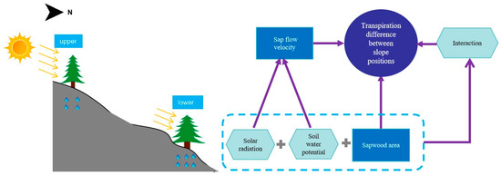
Figure 1.
The design scheme of main factors controlling transpiration differences between different positions (the number of yellow arrows represents the intensity of solar radiation density, the amount of water droplets indicates the soil moisture conditions, and the size of the trees corresponds to the differences in sapwood area).
This study hypothesizes that the transpiration differences between the two plots are mainly caused by the differences in stand structure, terrain shading, and soil water potential. The difference in stand structure is mainly reflected in the sapwood area, and its effect can be quantitatively represented by the product of sapwood area and sap flow velocity when calculating stand transpiration. The sap flow velocity is defined as the amount of transpired water passing through a unit of sapwood area per unit time; thus, it is not related to the effect of stand structure, but the difference in average daily sap flow velocity () between the lower slope plot () and the upper slope plot () is assumed to be composed of the effects of differences in terrain shading () and soil water potential () as described below:
Therefore, a technical challenge is how to separate the contributions of the differences in terrain shading and soil water potential to the difference in sap flow velocity between the two plots from the measured data and how to calculate the contributions to the differences in transpiration between the two plots based on the production of sapwood area.
Due to the complex interplay of soil water potential, slope gradient, and terrain shading from surrounding slopes, there can be various permutations in the relative magnitudes of sap flow velocity between the two plots (Figure 2). Generally, the upper slope plot, being less obstructed by terrain shading, exhibits an earlier onset and later cessation of diurnal sap flow activity (indicated by the dashed line in Figure 2a). Under cloudless conditions, the peaks of intra-daily sap flow velocity usually appear around noon, when the effect of terrain shading is minimal, which allows both plots to receive roughly equal solar radiation, especially during the summer, when the solar altitude angle is substantial, potentially reducing their solar radiation difference to zero [46]; hence, the distinction in sap flow velocity peaks (Points A and B in Figure 2a) between the upper and lower slope plots is primarily caused by the difference in soil water potential between the two plots.
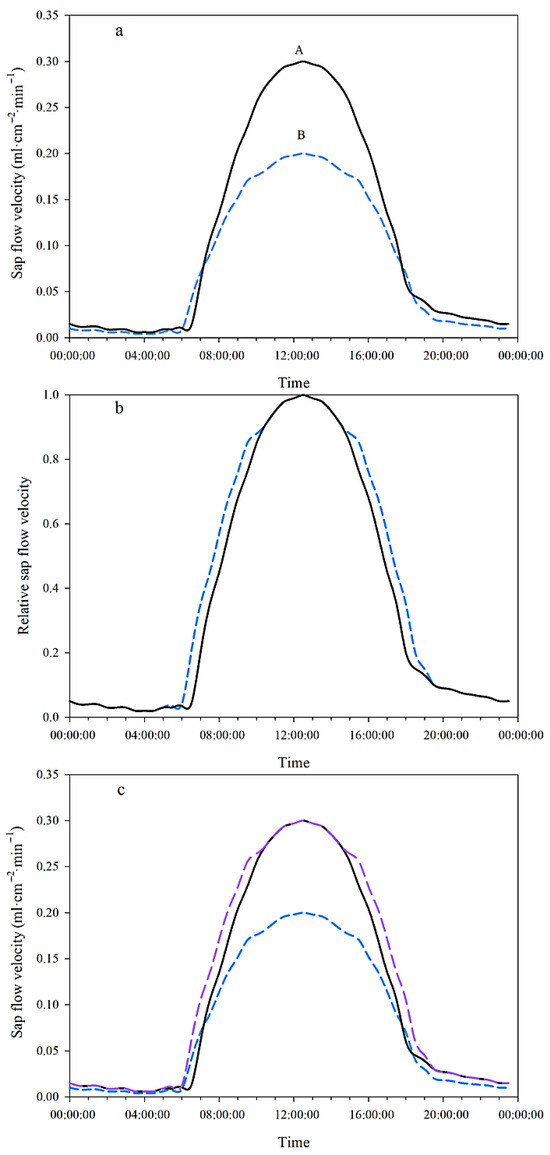
Figure 2.
Schematic diagram of distinguishing the effects of the differences in terrain shading and soil water potential on the difference in sap flow velocity between upper (blue dashed line, B) and lower slope plot (black solid line, A)—(a): actual measured sap flow velocity; (b): relative sap flow velocity; (c): actual measured sap flow velocity and the ideal sap flow velocity at the lower slope plot under the hypothesis of no difference in terrain shading compared to the upper slope plot (purple dashed line).
To separate the effect of terrain shading differences on sap flow velocity variation without disturbances from weather events such as cloud cover, only the data from sunny days were analyzed. Firstly, Equation (4) was used to calculate the ratios of instantaneous sap flow velocity (, mL·cm−2·min−1) to its daily peak value (, mL·cm−2·min−1) as relative sap flow velocity () for each plot throughout the day (Figure 2b):
where is the dimensionless relative sap flow velocity of plot i (i = U for upper slope plot or i = L for lower slope plot) at moment j (the time when sap flow velocity is recorded), is the instantaneous sap flow velocity of plot i at moment j, and is the maximum intra-daily sap flow velocity of plot i, typically occurring around noon.
If there were no differences in terrain shading between the upper and lower slope plots, the diurnal process of relative sap flow velocity of the lower slope plot should be exactly the same as that of the upper slope plot. Therefore, Equation (5) was used to calculate the ideal sap flow velocity of the lower slope plot under the hypothetical condition of no difference in terrain shading between the two plots, as shown by the outermost purple dashed line in Figure 2c:
The instantaneous difference in sap flow velocity caused by the terrain shading differences () between the two plots is equal to the difference between the ideal sap flow velocity of the lower slope plot (, mL·cm−2·min−1) and the actually measured sap flow rate of the lower slope plot (). This is represented by the difference between the outermost purple dashed line and the middle black solid line in Figure 2c:
The instantaneous difference in sap flow velocity caused by soil water potential differences () between the two plots is given by Equation (7), This is represented by the difference between the outermost purple thick dashed line and the innermost blue dashed line in Figure 2c:
Using Equations (5)–(7), which calculate the ideal sap flow velocity at the lower slope plot under the hypothesis of no difference in terrain shading compared to the upper slope plot, the instantaneous sap flow velocity differences caused by the differences in terrain shading and soil water potential between the two plots can be calculated. Then, it is straightforward to compute the daily means of , , and .
The daily transpiration at the upper (TU) and lower slope (TL) plots is calculated with Equations (8) and (9):
where (m2) is the sapwood of the upper plot, (m2) is the difference in sapwood between the upper and lower plots, and (m2) is the horizontal area of the plot.
Assuming that the daily transpiration difference (, mm) between the two plots is the sum of the transpiration differences caused by the differences in terrain shading (), soil water potential (), sapwood area (), and the interactive effects of the three factors (), this can be expressed by Equation (10):
, , , and could be calculated using following equations:
Using the above equations, the contributions of the three factors and their interactions to the daily transpiration differences between the upper and lower slope plots can be separated based on the daily observation data. By summing the values of each day of the study period, the contributions of each factor and their interactions to the overall transpiration differences in the whole growing season can be obtained. Because the upper slope plot is used as a reference, a positive or negative value of , , , and indicates a promotion or limitation effect on the transpiration at the lower slope plot, respectively.
To minimize the noise interference in the sap flow analysis, especially on rainy days [46], the days with data missing and the rainy days were excluded from the analysis. In total, 33 days were excluded, leaving only 59 days to form the dataset for analysis. The data analysis was conducted using SigmaPlot (v14.0) and R (v4.0.2).
3. Results
3.1. Environmental Conditions
The average daily air temperature during the study period was 15.9 °C, with the highest one of 34.4 °C on 25 July and the lowest one of 0.4 °C on 30 September (Figure 3a). The average daily solar radiation intensity was 133.8 W·m−2, ranging from 15.4 to 214.7 W·m−2 (Figure 3b). The average VPD was 1.37 kPa, reaching its maximum of 2.64 kPa on July 27 (Figure 3c). The precipitation during the study period (from July to September 2015) amounted to only 188 mm (Figure 3d), as a drought year, which was significantly lower than the average (372 mm) from 2010 to 2014, but 60% (112 mm) was concentrated in September, while the rainfall in July (27 mm) and August (49 mm) was significantly less than that in previous years (with averages of 158 mm in July and 116 mm in August from 2010 to 2014). There were only three days (3 August, 3 September, and 16 September) with daily rainfall exceeding 20 mm.
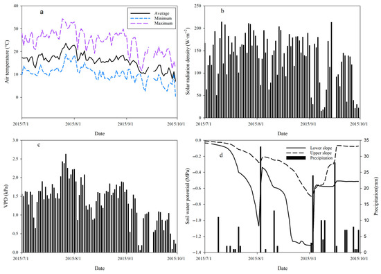
Figure 3.
Variation in environmental factors—(a): air temperature; (b): solar radiation intensity; (c): VPD; (d): soil water potential and precipitation—during study period.
The soil water potential of the 0–60 cm layer (ψ0–60, MPa) exhibited a similar variation trend for both plots (Figure 3d), showing a significant rebound only after two rainfall events on 3 August (33 mm) and 3 September (27 mm). During the entire study period, the average soil water potential was −0.582 MPa at the upper slope plot, which was very significantly (p < 0.01) lower than the value of −0.240 MPa at the lower slope plot.
3.2. The Difference in Sap Flow Velocity Between Two Plots
The intraday variation in sap flow velocity at both plots exhibits a unimodal curve, with a significantly higher peak value at the lower slope plot than at the upper slope plot (Figure 4). The daily averages of peak sap flow velocity at the upper slope plot were 0.138, 0.070, and 0.078 mL·cm−2·min−1 in July, August, and September, respectively, while these were 0.154, 0.120, and 0.114 mL·cm−2·min−1 at the lower slope plot. In the whole study period, the average daily sap flow velocity at the lower slope plot was 0.051 mL·cm−2·min−1, which was significantly (p < 0.01) higher than the value of 0.037 mL·cm−2·min−1 at the upper slope plot. Additionally, there was a weak nocturnal sap flow at both plots, and it was higher at the lower slope plot than at the upper slope plot. The nocturnal sap flow was mainly caused by the insufficient supply of soil water during the daytime, which led to the water deficit of the tree trunk in the daytime and recharge in the nighttime. The nocturnal sap flow velocity was dependent on the soil moisture conditions.
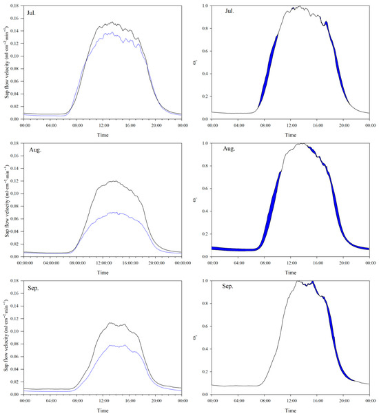
Figure 4.
The intraday variation in monthly average sap flow velocity at upper (blue lines) and lower (black lines) slope plots (left), and the intraday variation in monthly average relative sap flow velocity at upper and lower slope plots (right) (blue shadowed area: the period of higher monthly relative sap flow velocity at the upper slope plot than at the lower slope).
3.3. The Sap Flow Velocity Difference Driven by Terrain Shading Difference
The difference in the daily averages of the relative sap flow velocity in July, August, and September (see Equation (4)) between the two plots is shown in Figure 4 as the blue shadowed area. Because this difference was caused by the terrain shading difference between the two plots according to the definition in this study, the intraday process of the monthly averages for relative sap flow velocity was basically the same for both plots in the time period around noon when the solar altitude angle is at its maximum. Notably, the phenomena of higher monthly relative sap flow velocity at the upper slope plot than at the lower slope appeared in the periods of 7:05–10:10 and 15:30–20:30 in July, 6:05–10:35 and 14:10–20:15 in August, and 13:40–19:35 in September.
The daily sum of the difference in relative sap flow velocity () between the two plots was 4.67 in July, 6.47 in August, and 2.39 in September, and the daily average of the difference in relative sap flow velocity between the two plots was 0.049, 0.052, and 0.033, respectively. It can be seen from Figure 4 that the duration of terrain shading at the lower slope plot and the consequent limitation of the daily average relative sap flow velocity were less in July than in August. Furthermore, in September, the phenomena of lower relative sap flow velocity at the lower slope plot than at the upper slope plot appeared only in the afternoon (Figure 4).
The effect of terrain shading on reducing the sap flow velocity at the lower slope plot exhibited an overall decreasing trend in the study period, with a peak value of 0.008 mL·cm−2·min−1 on 5 August (Figure 5) and a z-value of −2.33 (p = 0.0199) from a Mann–Kendall trend test. The fluctuation was mainly caused by the scattered changes in solar radiation on cloudy or overcast days. Over the entire study period, the average reduction in sap flow velocity by terrain shading () at the lower slope plot was 0.003 mL·cm−2·min−1, constituting 5.31% of the ideal sap flow velocity at the lower slope plot. Further analysis showed that the sap flow velocity reduction at the lower slope plot by terrain shading correlated linearly and positively with solar radiation intensity (Figure 6).
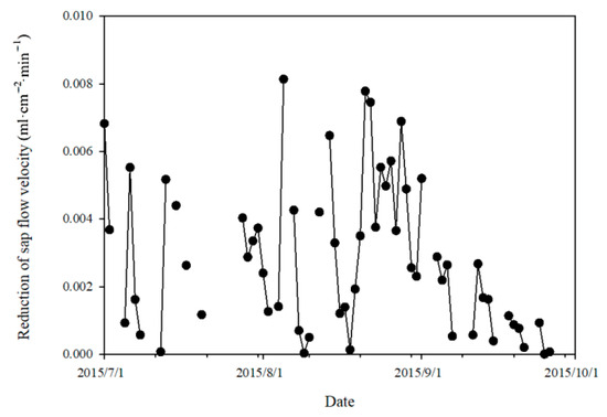
Figure 5.
Variation in daily reduction of sap flow velocity at lower slope due to terrain shading.
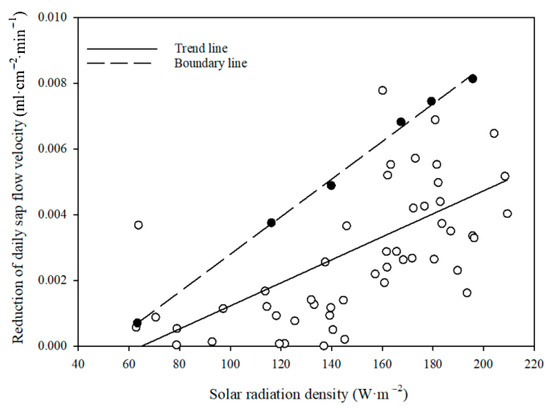
Figure 6.
Variation in daily reduction of sap flow velocity due to terrain shading at lower slope plot with solar radiation intensity (hollow circle: daily reduction of sap flow velocity at lower slope due to terrain shading; solid circle: daily reduction of sap flow velocity at lower slope due to terrain shading were used for upper boundary line).
3.4. The Sap Flow Velocity Difference Driven by Soil Water Potential Difference
During the study period, the sap flow velocity reduction caused by the lower soil water potential at the upper slope plot showed a variation trend of firstly increasing and then decreasing and then increasing again (Figure 7), and the Mann–Kendall trend test result showed a z-value of 2.52 (p = 0.012).
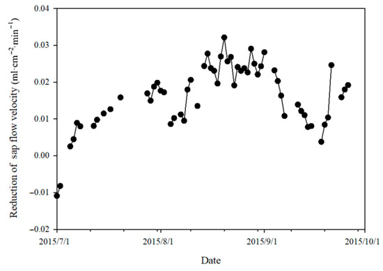
Figure 7.
Variation in the daily sap flow velocity reduction at upper slope plot caused by its lower soil water potential than at lower slope plot.
From 1 July to 3 September, the reduction in sap flow velocity increased gradually at the upper slope plot mainly due to its decreasing soil water potential (Figure 3d) but also due to the high level of VPD, which led to high transpiration demand in this period. The fluctuation of sap flow velocity reduction was primarily induced by the occasionally appearing higher air humidity of cloudy days or in overcast periods.
From 4 to 18 September, there was a decrease in the reduction of sap flow velocity caused by the lower soil water potential at the upper slope plot than at the lower slope plot. This can be explained by the decrease in the soil water potential difference between the two plots due to the higher recovery of soil moisture at the upper slope plot after the rainfall events after 3 September and by the lowered VPD and transpiration demand.
From 19 to 30 September, the stable but obviously lower soil water potential at the upper slope plot than at the lower slope plot and the relatively higher VPD and transpiration demand together led to an increase in the reduction of sap flow velocity at the upper slope plot compared to the lower slope plot, i.e., an increase in the limitation of the sap flow velocity by the soil water potential difference.
In the entire study period, the average sap flow velocity reduction at the upper slope plot () due to its lower soil water potential compared to the ideal sap flow velocity at the lower slope plot was 0.017 mL·cm−2·min−1. This constituted 48.20% of the ideal sap flow velocity at the lower slope plot over the study period. The sap flow velocity reduction at the upper slope plot showed a quadratic function relation to the difference in soil water potential between the two plots (Figure 8). This means that a higher soil water potential difference between the two plots led to a higher limitation effect on the sap flow velocity at the upper slope plot due to stronger soil drought stress.
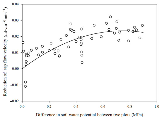
Figure 8.
Variation in daily sap flow velocity reduction at upper slope with the soil water potential difference between the upper and lower slope plots.
3.5. Contributions of Individual Factors to the Transpiration Difference Between Two Plots
The daily stand transpiration at both slope positions exhibited a progressive decrease trend in the study period (Figure 9). The Mann–Kendall trend test results showed a z-value of −5.06 at the upper slope and −5.41 at the lower slope (p < 0.001). This pattern was mainly attributed to the relatively scant rainfall in July and August, which led to a gradual decrease in soil water potential (Figure 3d) and the consequent limitation of transpiration. There was a partial recovery of the soil water potential in September owing to rainfall replenishment, but this led to only a small recovery of the daily stand transpiration. This can be explained by the reduced PET due to decreased air temperatures and the inherent restriction imposed by trees’ seasonal growth patterns.
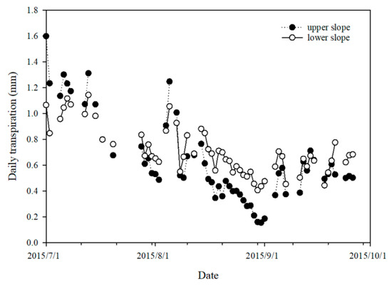
Figure 9.
The variation in daily stand transpiration at the upper and lower slope plots.
Over the study period, the daily stand transpiration at the lower slope plot was generally higher than that at the upper slope plot, with an average of 0.71 and 0.63 mm·day−1 and a sum over 59 days of 41.91 and 37.38 mm, respectively. This denotes a net difference of 4.53 mm in the measured stand transpiration between the two plots.
Figure 10 illustrates the separated contributions of the differences in sapwood area, solar radiation, soil water potential, and their interactions to the daily stand transpiration difference between the two plots when taking the upper slope plot as the reference. A promotion effect was found for the soil moisture difference (higher soil moisture at the lower slope plot than at the upper slope plot), while a limitation effect was found for the sapwood area difference, terrain shading, and the interactions of the three factors.
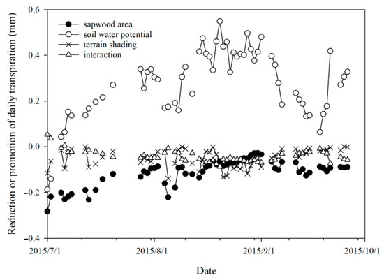
Figure 10.
Variation in contributions of main factors to the daily transpiration difference between two plots.
The limitation effect by the solar radiation difference (terrain shading), calculated using Equation (11), had an average (range) of 0.05 (0–0.14) mm·day−1, and it showed a decreasing trend and tended to stabilize but with frequent fluctuations (Figure 10). This was mainly caused by the seasonal variation in the solar radiation difference between the two plots and the shift in sunrise and sunset directions, together with the distribution of cloudy and overcast weather throughout the study period.
The promotion effect by the soil water potential difference between the two plots, calculated using Equation (12), had an average (range) of 0.28 (0.04–0.55) mm·day−1, and it showed a variation pattern of firstly increasing and then decreasing with some fluctuations. In July and August, the scarcity of rainfall led to a fast increase in the soil water potential difference and consequent transpiration differences between the two plots. However, the diminishment of the soil water potential difference by several big rainfall events in early August and early and mid-September, together with the suppression of VPD and evaporation demand due to the extended cloudy or overcast or rainy weather from 3 to 18 September, decreased the transpiration difference between the two plots.
The limitation effect by the sapwood area difference, calculated using Equation (13), had an average (range) of 0.11 (0.03–0.28) mm·day−1, and it showed a trend of first decreasing and then gradually leveling off (Figure 10). This variation trend was mainly attributable to the gradual decrease in the sap flow velocity at the upper slope plot during the study period.
The interactive effects of the three factors on the daily transpiration at the lower slope plot, calculated using Equation (14), primarily manifested as a small and steady limitation, except for the few days of 1, 2, and 6 July, when they exhibited a small promotion effect. The interactive effects of the three factors had an average (range) of −0.04 (−0.09~0.005) mm·day−1.
Figure 11 presents the reduction or promotion effects of the main factors and their interaction on the total transpiration of the 59 days studied at the lower slope plot compared to that at the upper slope plot. Only the higher soil water potential at the lower slope plot exerted a promotion effect of 16.40 mm, while the lower sapwood area and lower solar radiation at the lower slope plot as well as the interaction of three factors exerted a reduction effect of −6.61, −2.86, and −2.40 mm, respectively. Owing to the offsetting effects of these four contributions, the total transpiration for the 59 days studied at the lower slope plot was only 4.53 mm higher than that at the upper slope plot. The sum of the absolute effects of the three factors and their interaction amounted to 28.27 mm. The ratio of the absolute effect of each contributor to their sum can be used to assess their contributions, showing a ranking as follows: soil moisture (soil water potential difference, 58.0%) > stand structure (sapwood area difference, 23.4%) > solar radiation (terrain shading, 10.1%) > interaction of the three factors (8.5%).
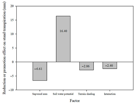
Figure 11.
The reduction or promotion effects of main factors and their interaction on the total transpiration of the 59 days studied at the lower slope plot compared to the upper slope plot.
4. Discussion
4.1. Differences in Sap Flow Velocity Among Slope Positions
The difference in sap flow velocity among slope positions is an important factor determining the stand transpiration variation across slopes and can be decisive when the sapwood area is similar or comparable. In this study, the sap flow velocity was significantly higher at the lower slope plot than at the upper slope (p < 0.01). The same result can be found in numerous studies: One was conducted in the Hudson Highlands of New York State, USA, (with annual precipitation of 1190 mm) on slopes growing both drought-tolerant and moist ecological types of Quercus rubra L. stands [47]; another one was a study of Toona ciliata var. pubescens plantations in Kaihua County of Zhejiang Province, China [48]. Another example was the study carried out in the Ochozu experimental watershed in western Japan, which showed that the sap flow velocity of Japanese cypress (Chamaecyparis obtusa) stands at the upper slope was usually only 70% of that at the lower slope [20]. However, the study on the transpiration of Japanese cedar (Cedar japonica) on Kyushu Island in Japan [21,46] and studies on the whole-tree transpiration of quaking aspen (Populus tremuloides Michx), speckled alder (Alnus incana Spreng), and white cedar (Thuja occidentalis L.) in Park Falls of Wisconsin, USA [49], did not show significant differences in sap flow velocity across slope positions. A study of transpiration patterns and water use strategies for beech (Fagus sylvatica L.) and oak (Quercus petraea (Matt.) Lieb. x robur) trees along a hillslope in Luxembourg revealed that, for the average DBH class (25–50 cm), beech trees exhibited consistently higher daily mean sap velocities at mid-slope compared to other slope positions. By contrast, no significant difference was observed in sap flow velocity for beech trees from the large DBH class (50–75 cm) across sampling areas. Notably, oak trees demonstrated significantly elevated sap flow velocity at the plateau (top slope) for both DBH classes when compared to other slope positions [50]. Research on the impact of topography on the water use of beech trees under different climate types has shown that, in the Weierbach catchment (oceanic climate), the sap flow velocity was significantly higher (p < 0.001) at the mid-slope location than at the plateau and footslope, but in the Lecciona catchment (Mediterranean climate), there were no statistical differences in the overall mean sap flow velocity among locations [51]. A study of Larch plantations on a long slope in the semi-humid area of the Liupan Mountains in northwest China revealed that the sap flow velocity followed the order of middle-upper slope, middle-lower slope, middle slope, lower slope, and upper slope. Generally, in the humid region, where soil moisture is sufficient, there are no significant differences in sap flow velocity among slope positions. Sometimes, the sap flow velocity at the slope top may even be higher due to the impact of transpiration demand. However, in arid and water-scarce areas, where soil moisture is low, the sap flow velocity at the lower slope is generally higher than that at the upper slope. Meanwhile, the difference in water use strategy among tree species may also be a cause of the sap flow velocity difference among slope positions. The divergent variation patterns of sap flow velocity along slope positions observed in different studies are the integrated result of many driving factors, mainly climate type and soil moisture differences along slope positions. This study was conducted in the semiarid area with a mean annual precipitation of only 449 mm; thus, the factors/processes affecting the soil water availability to plants played a critical role. For example, the redistribution of rainwater through surface runoff and interflow and the increased soil thickness and corresponding water storage capacity at the lower slope positions jointly led to the higher soil water potential of the 0–60 cm soil layer at the lower slope plot compared with the upper slope plot, especially during drier periods. The studies of Kumagai et al. [21,46] and Loranty et al. [49] also showed higher soil water potential at lower slope positions in the soil layers of 0–20 cm and 0–6 cm, although the mean annual precipitation of these two studies was as high as 2150 and 810 mm, respectively, and this might have led to a high soil water potential across the slope such that the soil water potential difference was unable to make a significant transpiration difference [49], because transpiration can be significantly reduced only when the relative extractable soil water (REW) is <0.4 [52,53,54], also in the same area of this study [44].
The variation in between the two plots across the different months was influenced by the seasonal variation in the sunrise/sunset direction in the study period, as well as weather conditions. In the Northern Hemisphere, from the summer solstice to the winter solstice, the sunrise direction shifts gradually from the northeast to the southeast, while the sunset direction shifts gradually from the northwest to the southwest. The duration of terrain shading at the lower slope plot and the consequent limitation of the daily average relative sap flow velocity were less in July than in August (Figure 4); that is primarily because the proportion of cloudy or overcast days in July (53.3%) was significantly higher than that in August (33.3%). Furthermore, in September, the phenomena of smaller relative sap flow velocity at the lower slope plot than at the upper slope plot appeared only in afternoon (Figure 4); this can be explained by the fact that both plots on the northwest-facing slope received direct sunlight almost simultaneously when the sun rose from the southeast in September.
A similar study quantifying the sap flow velocity differences of larch plantations along a slope and the causes was conducted in the semi-humid area of the Liupan Mountains. It showed that the sap flow velocity difference was determined jointly by the slope-position effect and terrain shading effect, and it verified that the sap flow velocity was affected by both effects at the slope foot plot but only by the slope-position effect at mid-slope and top-slope plots. That study assumed that the terrain shading effect was induced by the differences in PET and LAI caused by terrain shading and that the slope-position effect was induced by the differences in PET, soil moisture, and LAI caused by slope position. The main causes of the sap flow velocity differences along the slope in that study were not the same as those in our study, probably due to the differences in climate, slope aspect, and length; terrain shading from the neighboring hillslope; soil thickness and hydrological properties, etc.; and the analysis methods used in these two studies.
4.2. Differences in Stand Transpiration Along Slope Positions
The total stand transpiration for the 59 days selected in this study was higher at the lower slope plot (41.91 mm) than at the upper slope plot (37.38 mm). This is consistent with studies on the slope-position differences in the stand transpiration of Japanese cedar [46] and Japanese cypress in Japan [20] and the evapotranspiration of mixed eucalyptus forests in Australia [55].
The difference in stand transpiration among slope positions varied in previous studies due to the varying effects of multiple factors. For example, in a Japanese cedar forest with a humid climate [46,56], the sap flow velocity was essentially the same at any slope position in the growing season because there was no soil moisture limitation of transpiration, and the main cause of the higher transpiration at the lower slope than at the upper slope was the higher sapwood area at the lower slope (46.0 m2·ha−1) than at the upper slope (36.3 m2·ha−1); thus, the difference in transpiration across slope positions was mainly explained by the difference in stand sapwood area (Ridge 11.7, Mid-slope 26.1 and Riparian 25.1 m2·ha−1) rather than by the difference in sap flow velocity [56]. In the mixed eucalyptus forests with an annual precipitation of 1098 mm in northeast Melbourne in Australia, the transpiration at the upper slope was about 40% lower than that at the lower slope [55], which was mainly caused by the stand structure differences of the higher sapwood area and LAI at the lower slope than at the upper slope due to the different soil type and soil thickness along the slope positions. In an eastern white pine (Pinus strobus L.) stand, the greatest cause of transpiration variability among plots was also the sapwood area variation [23]. However, the differences in both sapwood area and sap flow velocity were the causes of the transpiration differences between the upper and lower slope plots [20], where the transpiration at the upper slope was about 50% less than that at the lower slope due to the 30% smaller sapwood area and 23% lower sap flow velocity at the upper slope than at the lower slope. In a forest of Rhus chinensis in the humid karst terrain in southwest China, the transpiration rate and amount at the uphill position were as low as nearly half of that at the downhill position, mainly because of the lower mean soil water content at the uphill position of around 60% of that at the downhill position [57]. In summary, the main causes of stand transpiration differences among slope positions can be the differences in sapwood area, LAI, soil water content, and sap flow velocity in humid regions.
In contrast to the above-mentioned studies in humid climates, this study site had a semiarid climate; thus, the difference in soil water potential played a key role in the transpiration difference among slope positions. Variations in microclimate, soil thickness, and water storage capacity, as well as the redistribution of rainwater through surface runoff and interflow along slope positions, often led to more severe soil drought stress at the upper slope than at the lower slope. In this study, the most important factor influencing the transpiration difference was the soil water potential difference. The higher soil water potential at the lower slope plot had a promoting effect of an absolute contribution of 16.4 mm, accounting for 58.0% of the total (28.27 mm) of the absolute impacts of the three factors and their interaction. The second important factor influencing the transpiration difference was the significant difference in sapwood area. The lower sapwood area at the lower slope plot (Table 1) had a limitation effect of 6.61 mm on the transpiration, accounting for 23.4% of the total of the absolute impacts. The third important factor influencing the transpiration difference was the terrain shading (solar radiation), which led to a transpiration reduction of 2.86 mm, accounting for 10.1% of the total of the absolute impacts. Additionally, the interaction of the three factors had a limitation effect on the transpiration at the lower slope plot, with a value of 2.40 mm, accounting for 8.5% of the total of the absolute impacts.
4.3. Limitations of This Study and Recommendations for Future Research
A deep understanding and the accurate prediction of stand transpiration along slope positions are required for the up-scaling of transpiration from a stand plot to the whole slope. This study indicates that the forest transpiration difference among slope positions in semiarid areas is an integrated result of the offsetting impacts of multiple factors and their interaction, with the magnitude ordering of the absolute impacts as follows: soil water potential > sapwood area > terrain shading > interaction. The factor of soil water potential exerted a promotion effect while others exerted a reduction effect on the stand transpiration at the lower slope plot when compared with that at the upper slope plot.
However, this study was conducted on one typical slope and within few months, thus with some obvious limitations: (1) Some landform factors (e.g., slope length, aspect, gradient, and the shading effect from neighbor slopes) and soil factors (e.g., soil type, texture, thickness, porosity, and water storage capacity), which vary among slopes and areas and may influence stand transpiration, were not considered in this study. More studies should be carried out on more slopes with varying characteristics to consider the impacts of these factors. (2) This study compared the differences in sap flow velocity and transpiration only between a lower slope plot and a higher slope plot, and the successive variation in transpiration and influencing factors were not considered. In future studies, more stand plots along slope positions should be set up to understand the successive spatial variations in stand transpiration response to multiple factors. (3) It is very likely that the effect size and order of the influencing factors may vary with changing conditions of climate, landform, soil, and vegetation. Therefore, continuous monitoring of the stand transpiration process and influencing factors on more typical slopes should be encouraged in the future, for example, to reflect the effect of varying precipitation and its temporal distribution. (4) A general and quantitative rule about the variation in stand transpiration along slope positions and its response to various influencing factors cannot be drawn from this study, which involved only two plots within a limited time period. Therefore, quantitative and longer-term studies and process-based model development and application should be promoted, alongside fundamental studies with analytical methods, for the precise prediction of forest transpiration and to guide integrated forest–water management under changing conditions across multiple spatial and temporal scales.
5. Conclusions
This pilot study on the stand transpiration of larch plantations in the semiarid area of the Liupan Mountains in northwest China showed that the difference in stand transpiration exists along slope positions due to the integrated and mutual offsetting impacts of multiple factors and their interaction. The separated contributions of the influencing factors followed the order of soil water potential > sapwood area > terrain shading > interaction of the three factors. The higher soil water potential at the lower slope plot than at the upper slope plot exerted a dominant promotion effect on the transpiration at the lower slope plot, while the other factors and their interaction exerted a reduction effect on the transpiration at the lower slope plot. The promotion effect was larger than the sum of the three reduction effects, leading to a higher daily average and total transpiration at the lower slope plot. In addition, the differences in stand transpiration increased with increasing differences in the three factors between the two plots. The accurate prediction of forest transpiration at the plot and slope scales through up-scaling requires a deep understanding and quantitative calculation of the impacts of main factors, especially in semiarid regions with obvious impacts of soil moisture and stand structure differences along slope positions. This study provides a theoretical basis for the accurate estimation of forest transpiration and evapotranspiration at the scope scale and scientific guidance for forest restoration on slopes in arid and water-scarce areas.
Author Contributions
Y.W. (Yanbing Wang): Conceptualization, Investigation, Methodology, Visualization, Writing—Original draft. Y.W. (Yanhui Wang): Conceptualization, Validation, Funding acquisition, Supervision, Writing—Review and editing. W.X. and Z.L.: Writing—Review and editing. T.Z., Y.Y., X.H. and H.R.: Data curation, Investigation. All authors have read and agreed to the published version of the manuscript.
Funding
This work was funded by the National Natural Science Foundation of China (U20A2085, U21A2005), the Liupanshan Forestry Bureau-commissioned project “Monitoring the ecological restoration effectiveness of degraded plantations in 2023”, and the Central Public-Interest Scientific Institution Basal Research Fund of the Chinese Academy of Forestry (CAFYBB2021ZW002).
Data Availability Statement
The data presented in this study are available on request from the corresponding author.
Conflicts of Interest
The authors declare no conflicts of interest.
References
- Allan, R.; Barlow, M.; Byrne, M.P.; Cherchi, A.; Douville, H.; Fowler, H.J.; Gan, T.Y.; Pendergrass, A.G.; Rosenfeld, D.; Swann, A.L.S.; et al. Advances in Understanding Large-Scale Responses of the Water Cycle to Climate Change. Ann. N. Y. Acad. Sci. 2020, 1472, 49–75. [Google Scholar] [CrossRef]
- Jiang, F.; Xie, X.; Wang, Y.; Liang, S.; Zhu, B.; Meng, S.; Zhang, X.; Chen, Y.; Liu, Y. Vegetation greening intensified transpiration but constrained soil evaporation on the Loess Plateau. J. Hydrol. 2022, 614, 128514. [Google Scholar] [CrossRef]
- Cui, Z.; Zhang, Y.; Wang, A.; Wu, J. Forest evapotranspiration trends and their driving factors under climate change. J. Hydrol. 2024, 644, 132114. [Google Scholar] [CrossRef]
- Lian, X.; Piao, S.; Huntingford, C.; Li, Y.; Zeng, Z.; Wang, X.; Ciais, P.; McVicar, T.R.; Peng, S.; Ottlé, C.; et al. Partitioning global land evapotranspiration using CMIP5 models constrained by observations. Nat. Clim. Change 2018, 8, 640–646. [Google Scholar] [CrossRef]
- Jasechko, S.; Sharp, Z.D.; Gibson, J.J.; Birks, S.J.; Yi, Y.; Fawcett, P.J. Terrestrial water fluxes dominated by transpiration. Nature 2013, 496, 347–350. [Google Scholar] [CrossRef] [PubMed]
- Shuttleworth, W.J. Evaporation from Amazonian rainforest. Proc. R. Soc. Lond. B 1988, 233, 321–346. [Google Scholar] [CrossRef]
- McJannet, D.L.; Wallace, J.S.; Fitch, P.; Disher, M.; Reddell, P. Water balance of tropical rainforest canopies in north Queensland, Australia. Hydrol. Process. 2007, 21, 3473–3484. [Google Scholar] [CrossRef]
- Su, J.P.; Kang, B.W. Research Proceeding of Trees Transpiration in China. Res. Soil Water Conserv. 2004, 11, 177–179+186. [Google Scholar] [CrossRef]
- Lloyd, J.; Grace, J.; Miranda, A.C.; Meir, P.; Wong, S.C.; Miranda, H.S.; Wright, I.R.; Gash, J.H.C.; McIntyre, J. A simple calibrated model of Amazon rainforest productivity based on leaf biochemical properties. Plant Cell Environ. 1995, 18, 1129–1145. [Google Scholar] [CrossRef]
- Hanba, Y.T.; Noma, N.; Umeki, K. Relationship between leaf characteristics, tree sizes and species distribution along a slope in a warm temperate forest. Ecol. Res. 2000, 15, 393–403. [Google Scholar] [CrossRef]
- Luizao, R.C.C.; Luizao, F.J.; Paiva, R.Q.; Monteiro, T.F.; Sousa, L.S.; Kruijt, B. Variation of carbon and nitrogen cycling processes along a topographic gradient in a central Amazonian forest. Glob. Change Biol. 2004, 10, 592–600. [Google Scholar] [CrossRef]
- Enoki, T.; Inoue, T.; Tashiro, N.; Ishii, H. Aboveground productivity of an unsuccessful 140-year-old Cryptomeria japonica plantation in northern Kyushu, Japan. J. For. Res. 2011, 16, 268–274. [Google Scholar] [CrossRef]
- Tateno, R.; Hishi, T.; Takeda, H. Above- and belowground biomass and net primary production in a cool-temperate deciduous forest in relation to topographical changes in soil nitrogen. For. Ecol. Manag. 2004, 193, 297–306. [Google Scholar] [CrossRef]
- Tokuchi, N.; Takeda, H.; Yoshida, K.; Iwatsubo, G. Topographical variations in a plant–soil system along a slope on Mt Ryuoh, Japan. Ecol. Res. 1999, 14, 361–369. [Google Scholar] [CrossRef]
- Grande, M.M.; Kaffas, K.; Verdone, M.; Borga, M.; Cocozza, C.; Dani, A.; Errico, A.; Fabiani, G.; Gourdol, L.; Klaus, J.; et al. Seasonal meteorological forcing controls runoff generation at multiple scales in a mediterranean forested mountain catchment. J. Hydrol. 2024, 639, 131642. [Google Scholar] [CrossRef]
- Yu, P.T. Application of physically-based distributed models in forest hydrology. For. Res. 2000, 13, 431–438. [Google Scholar] [CrossRef]
- Komatsu, H.; Kang, Y.; Kume, T.; Yoshifuji, N.; Hotta, N. Transpiration from a Cryptomeria japonica plantation, part 1: Aerodynamic control of transpiration. Hydrol. Process. 2006, 20, 1309–1320. [Google Scholar] [CrossRef]
- Komatsu, H.; Kang, Y.; Kume, T.; Yoshifuji, N.; Hotta, N. Transpiration from a Cryptomeria japonica plantation, part 2: Responses of canopy conductance to meteorological factors. Hydrol. Process. 2006, 20, 1321–1334. [Google Scholar] [CrossRef]
- Kumagai, T.; Aoki, S.; Nagasawa, H.; Mabuchi, T.; Kubota, K.; Inoue, S.; Utsumi, Y.; Otsuki, K. Sources of error in estimating stand transpiration using allometric relationships between stem diameter and sapwood area for Cryptomeria japonica and Chamaecyparis obtusa. Forest Ecol. Manag. 2005, 206, 191–195. [Google Scholar] [CrossRef]
- Kume, T.; Tsuruta, K.; Komatsu, H.; Shinohara, Y.; Katayama, A.; Ide, J.; Otsuki, K. Differences in sap flux-based stand transpiration between upper and lower slope positions in a Japanese cypress plantation watershed. Ecohydrology 2015, 6, 1105–1116. [Google Scholar] [CrossRef]
- Kumagai, T.; Aoki, S.; Shimizu, T.; Otsuki, K. Sap flow estimates of stand transpiration at two slope positions in a Japanese cedar forest watershed. Tree Physiol. 2007, 27, 161–168. [Google Scholar] [CrossRef] [PubMed]
- Wilson, K.B.; Hanson, P.J.; Mulholland, P.J.; Baldocchi, D.D.; Wullschleger, S.D. A comparison of methods for determining forest evapotranspiration and its components: Sap-flow, soil water budget, eddy covariance and catchment water balance. Agric. For. Meteorol. 2001, 106, 153–168. [Google Scholar] [CrossRef]
- Ford, C.R.; Hubbard, R.M.; Kloeppel, B.D.; Vos, J.M. A comparison of sap flux-based evapotranspiration estimates with catchment-scale water balance. Agric. For. Meteorol. 2007, 145, 176–185. [Google Scholar] [CrossRef]
- Ewers, B.E.; Mackay, D.S.; Gower, T.; Ahl, D.E.; Burrows, S.N.; Samanta, S.S. Tree species effects on stand transpiration in northern Wisconsin. Water Resour. Res. 2002, 38, w1103. [Google Scholar] [CrossRef]
- Ewers, B.E.; Gower, S.T.; Bond-Lamberty, B.; Wang, C.K. Effects of stand age and tree species on canopy transpiration and average stomatal conductance of boreal forests. Plant Cell Environ. 2005, 28, 660–678. [Google Scholar] [CrossRef]
- Mackay, D.S.; Ahl, D.E.; Ewers, B.E.; Gower, S.T.; Burrows, S.N.; Samanta, S.; Davis, K.J. Effects of aggregated classifications of forest composition on estimates of evapotranspiration in a northern Wisconsin forest. Glob. Change Biol. 2002, 8, 1253–1265. [Google Scholar] [CrossRef]
- Pataki, D.E.; Oren, R. Species differences in stomatal control of water loss at the canopy scale in a mature bottomland deciduous forest. Adv. Water Resour. 2003, 26, 1267–1278. [Google Scholar] [CrossRef]
- Bladon, K.D.; Silins, U.; LandhäUsser, S.M.; Lieffers, V.J. Differential transpiration by three boreal tree species in response to increased evaporative demand after variable retention harvesting. Agric. For. Meteorol. 2006, 138, 104–119. [Google Scholar] [CrossRef]
- Kumagai, T.; Aoki, S.; Nagasawa, H.; Mabuchi, T.; Kubota, K.; Inoue, S.; Utsumi, Y.; Otsuki, K. Effects of tree-to-tree and radial variations on sapflow estimates of transpiration in Japanese cedar. Agric. For. Meteorol. 2005, 135, 110–116. [Google Scholar] [CrossRef]
- Zang, D.; Beadle, C.L.; White, D.A. Variation of sap flow velocity in Eucalyptus globulus with position in sapwood and use of a correction coefficient. Tree Physiol. 1996, 16, 697–703. [Google Scholar] [CrossRef]
- Lu, P.; Müller, W.J.; Chacko, E.K. Spatial variations in xylem sap flux density in the trunk of orchard-grown, mature mango trees under changing soil water conditions. Tree Physiol. 2000, 20, 683–692. [Google Scholar] [CrossRef]
- Wullschleger, S.D.; King, A.W. Radial variation in sap velocity as a function of stem diameter and sapwood thickness in a yellow-poplar trees. Tree Physiol. 2000, 20, 511–518. [Google Scholar] [CrossRef] [PubMed]
- Delzon, S.; Sartore, M.; Granier, A.; Loustau, D. Radial profiles of sap flow with increasing tree size in maritime pine. Tree Physiol. 2004, 24, 1285–1293. [Google Scholar] [CrossRef]
- Granier, A.; Biron, P.; Bréda, N.; Pontailler, J.Y.; Saugier, B. Transpiration of trees and forest stands: Short and long-term monitoring using sapflow methods. Glob. Change Biol. 1996, 2, 265–274. [Google Scholar] [CrossRef]
- Wullschleger, S.D.; Hanson, P.J.; Todd, D.E. Transpiration from a multi-species deciduous forest as estimated by xylem sap flow techniques. For. Ecol. Manag. 2001, 143, 205–213. [Google Scholar] [CrossRef]
- Zhai, J.J.; Wang, L.; Liu, Y.; Wang, C.Y.; Mao, X.G. Assessing the effects of China’s three-north shelter forest program over 40 years. Sci. Total Environ. 2023, 857, 159354. [Google Scholar] [CrossRef] [PubMed]
- Wang, C.; Ouyang, H.; Maclaren, V.; Yin, Y.; Shao, B.; Boland, A.; Tian, Y. Evaluation of economic and social impacts of the sloping land conversion program: A case study in Dunhua County, China. Forest Policy Econ. 2012, 14, 50–57. [Google Scholar] [CrossRef]
- Zeng, Z.Z.; Peng, L.Q.; Piao, S.L. Response of terrestrial evapotranspiration to Earth’s greening. Curr. Opin. Environ. Sustain. 2018, 33, 9–25. [Google Scholar] [CrossRef]
- Fu, F.Y.; Wang, S.; Wu, X.T.; Wei, F.L.; Chen, P.; Grünzweig, J.M. Locating hydrologically unsustainable areas for supporting ecological restoration in China’s drylands. Earth’s Future 2024, 12, e2023EF004216. [Google Scholar] [CrossRef]
- Wang, Q.M.; Liu, H.Y.; Liang, B.Y.; Shi, L.; Wu, L.; Cao, J. Will large-scale forestation lead to a soil water deficit crisis in China’s drylands? Sci. Bull. 2024, 69, 1506–1514. [Google Scholar] [CrossRef]
- Zhou, J.X.; Wang, Y.Q.; Li, R.J.; He, H.R.; Sun, H.; Zhou, Z.X.; Zhao, Y.L.; Zhang, P.P.; Li, Z.M. Response of deep soil water deficit to afforestation, soil depth, and precipitation gradient. Agric. For. Meteorol. 2024, 352, 110024. [Google Scholar] [CrossRef]
- Gao, Y.Q. Present situation, existing problems and development suggestions of artificial coniferous forest in Liupan Mountain. Bull. Agric. Sci. Tech. 2023, 23, 7–9. [Google Scholar]
- Liu, Z.B. Spatio-temporal Variations and Scale Transition of Hydrological Impact of Larix principis-ruprechtii Plantation on a Slope of Liupan Mountains. Ph.D. Thesis, Chinese Academy of Forestry, Beijing, China, 2018; p. 120. [Google Scholar]
- Wang, Y.B.; Wang, Y.H.; Li, Z.H.; Han, X.S. Interannual variation of transpiration and its modeling of a larch plantation in semiarid northwest China. Forests 2020, 11, 1303. [Google Scholar] [CrossRef]
- Campbell, G.S.; Norman, J.M. Water Vapor and Other Gases. In An Introduction to Environmental Biophysics; Springer: New York, NY, USA, 1998; pp. 37–51. [Google Scholar] [CrossRef]
- Kumagai, T.; Tateishi, M.; Shimizu, T.; Otsuki, K. Transpiration and canopy conductance at two slope positions in a Japanese ceder forest watershed. Agric. For. Meteorol. 2008, 148, 1444–1455. [Google Scholar] [CrossRef]
- Engel, V.C.; Stieglitz, M.; Williams, M.; Griffin, K.L. Forest canopy hydraulic properties and catchment water balance: Observations and modelling. Ecol. Model. 2002, 154, 263–288. [Google Scholar] [CrossRef]
- Liu, J.; Chen, W.R.; Xu, J.L.; Zou, J.; Jiang, J.M.; Li, Y.J.; Diao, S.F. Trunk sap flow dynamic changes in response to the slopes of plantation of Toona ciliata var. pubescens. Chin. J. Appl. Ecol. 2014, 25, 2209–2214. [Google Scholar] [CrossRef]
- Loranty, M.M.; Mackay, D.S.; Ewers, B.E.; Adelman, J.D.; Kruger, E.L. Environmental drivers of spatial variation in whole-tree transpiration in an aspen-dominated upland-to-wetland forest gradient. Water Resour. Res. 2008, 44, W02441. [Google Scholar] [CrossRef]
- Fabiani, G.; Schoppach, R.; Penna, D.; Klaus, J. Transpiration patterns and water use strategies of beech and oak trees along a hillslope. Ecohydrology 2022, 15, e2382. [Google Scholar] [CrossRef]
- Fabiani, G.; Klaus, J.; Penna, D. Contrasting water use strategies of beech trees along two hillslopes with different slope and climate. Hydrol. Earth Syst. Sci. Discuss. 2023. in review. [Google Scholar] [CrossRef]
- Loustau, D.; Granier, A.; Bréda, N. A generic model of forest canopy conductance dependent on climate, soil water availability and leaf area index. Ann. For. Sci. 2000, 57, 755–765. [Google Scholar] [CrossRef]
- Sadras, V.O.; Milroy, S.P. Soil-water thresholds for the responses of leaf expansion and gas exchange: A review. Field Crop. Res. 1996, 47, 253–266. [Google Scholar] [CrossRef]
- Granier, A.; Bréda, N.; Biron, P.; Villette, S. A lumped water balance model to evaluate duration and intensity of drought constraints in forest stands. Ecol. Model. 1999, 116, 269–283. [Google Scholar] [CrossRef]
- Mitchell, P.J.; Benyon, R.G.; Lane, P.N.J. Responses of evapotranspiration at different topographic positions and catchment water balance following a pronounced drought in a mixed species eucalypt forest, Australia. J. Hydrol. 2012, 440–441, 62–74. [Google Scholar] [CrossRef]
- Tsuruta, K.; Yamamoto, H.; Kosugi, Y.; Makita, N.; Katsuyama, M.; Kosugi, K.; Tani, M. Slope position and water use by trees in a headwater catchment dominated by Japanese cypress: Implications for catchment-scale transpiration estimates. Ecohydrology 2020, 13, e2245. [Google Scholar] [CrossRef]
- Liu, W.; Nie, Y.; Luo, Z.; Wang, Z.; Huang, L.; He, F.; Chen, H. Transpiration rates decline under limited moisture supply along hillslopes in a humid karst terrain. Sci. Total Environ. 2023, 894, 164977. [Google Scholar] [CrossRef]
Disclaimer/Publisher’s Note: The statements, opinions and data contained in all publications are solely those of the individual author(s) and contributor(s) and not of MDPI and/or the editor(s). MDPI and/or the editor(s) disclaim responsibility for any injury to people or property resulting from any ideas, methods, instructions or products referred to in the content. |
© 2025 by the authors. Licensee MDPI, Basel, Switzerland. This article is an open access article distributed under the terms and conditions of the Creative Commons Attribution (CC BY) license (https://creativecommons.org/licenses/by/4.0/).