Monthly Diurnal Variations in Soil N₂O Fluxes and Their Environmental Drivers in a Temperate Forest in Northeastern China: Insights from Continuous Automated Monitoring

Abstract

Global warming, driven by increased greenhouse gas emissions, is a critical global concern. However, long-term trends in emissions remain poorly understood due to limited year-round data. The automated chamber method was used for continuous monitoring of soil N₂O fluxes in a mixed forest in Northeast China’s Changbai Mountains, analyzing monthly diurnal patterns and their relationships with soil temperature (Ts) and soil volumetric water content (VWC). The results revealed significant diurnal and seasonal variations, with peak emissions at 11:00 during the growing season (May–October) and elevated nighttime fluxes in winter (March, April, November, and December). The optimal sampling time was 14:00, closely reflecting daily mean fluxes. Soil Ts and VWC were key drivers, with seasonal variability in their effects: N₂O fluxes showed no significant relationship with Ts in January but strong correlations in February and March. The growing season Q₁₀ values ranged from 0.4 to 7.2 (mean = 2.5), indicating high-temperature sensitivity. Soil VWC effects were complex, with moderate VWC promoting denitrification and excessive VWC suppressing microbial activity. These findings provide critical insights for optimizing N₂O monitoring and improving emission estimates.

1. Introduction

Global warming and its associated ecological challenges have become a critical global concern, with rising greenhouse gas levels being a major contributor. While soil CO₂ emissions have been extensively studied, research on other greenhouse gases, particularly nitrous oxide (N₂O), remains limited, resulting in an incomplete understanding of soil greenhouse gas emissions. Notably, N₂O accounts for approximately 5% of the total global warming potential, as its radiative forcing strength per unit mass is 298 times greater than that of CO₂ over a 100-year period [1,2]. This highlights the need for deeper investigation into its emission mechanisms and influencing factors.

The chamber method is widely used for measuring soil greenhouse gas emissions (CO₂, CH₄, and N₂O), providing essential data for IPCC estimates of global terrestrial ecosystem emissions [3]. However, most N₂O flux measurements rely on static chambers with daily single sampling; appropriate sampling time selection is crucial for accurate daily average flux estimation [4,5]. Studies have shown significant N₂O emission increases during freeze–thaw cycles and precipitation events [6,7,8,9,10], underscoring the importance of sampling timing.

While prior studies have focused on monthly or seasonal data collection, annual datasets remain scarce, limiting our understanding of long-term emission trends. For example, optimal N₂O sampling times in wetlands vary monthly: 6:00 in June and December and 12:00 to 15:00 in April and October [11]. Forest ecosystem studies identify 6:00 and 10:00 as optimal sampling times [12,13], with peak emissions occurring from noon to evening [13,14] and troughs from early morning to dawn [13]. Methodological limitations and reliance on short-term data hinder the comprehensive characterization of long-term patterns. Continuous annual monitoring captures seasonal and interannual variability in N₂O fluxes, which helps to account for variability caused by environmental factors (e.g., temperature, precipitation and soil moisture). By integrating data over different time scales, annual monitoring reduces the uncertainty associated with single day measurements, thereby improving the reliability and representativeness of daily average estimates. Identifying critical sampling periods can enhance N₂O emission estimate accuracy and reduce temporal variability uncertainties, though differing optimal sampling times across studies indicate the need for further research.

Soil temperature and moisture are key factors regulating N₂O emissions [5,10,12,15,16,17,18,19,20]. Diurnally, N₂O fluxes are mainly influenced by soil temperature and microbial activity variations [21]. While increased soil temperature and moisture generally enhance N₂O emissions through stimulated microbial activity and nitrification/denitrification processes [12,13,22], some studies show that higher temperatures may cause water stress, inhibiting organic matter mineralization and reducing N₂O emissions [10,23,24]. Increased soil moisture can also suppress emissions in certain conditions [25,26,27], indicating complex emission mechanisms requiring further study.

This study expands annual-scale data analysis to monthly-scale analysis to optimize monitoring and prediction models, reveal seasonal variations, validate annual results, provide precise emission patterns, and enhance understanding of N₂O emission mechanisms. The objectives are to (1) examine monthly N₂O flux diurnal variations; (2) determine optimal daily sampling times, including peak and trough periods; and (3) analyze soil temperature (Ts) and soil volumetric water content (VWC) effects on N₂O fluxes and their correlations. The research aims to improve N₂O emission monitoring methods, enhance estimation accuracy, and support effective greenhouse gas mitigation strategies.

2. Materials and Methods

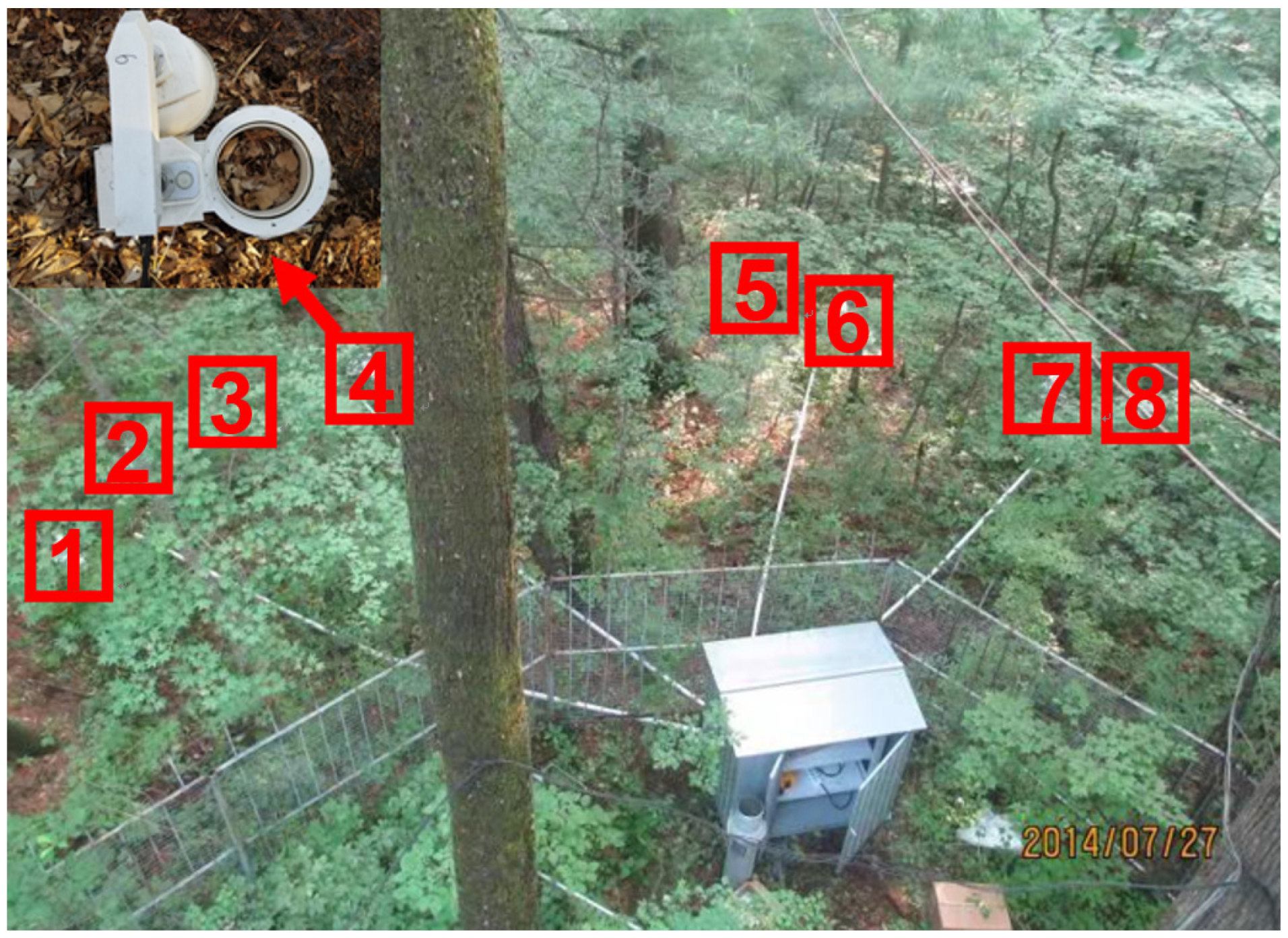
2.1. Study Site

The study was carried out in a mixed forest of broad-leaved Korean pine (42°24′9″ N, 128°05′45″ E, 738 m a.s.l.) located in the Changbai Mountains of northeastern China. As the Changbaishan Sample Site No. 1 in the reserve‘s core zone—a flagship temperate forest research station in China—this primary forest has remained undisturbed for over 200 years. The forest is dominated by Pinus koraiensis Sieb. et Zucc. with Tilia amurensis Rupr. and Quercus mongolica Fisch. ex Ledeb. as associated species [28] and displays four defining characteristics: (1) gentle topography (southwest-facing, 228.8° azimuth; mean slope 1.8°); (2) complex vertical stratification with 40% understory cover; (3) natural hydrological conditions (713 mm annual precipitation, with 5%–8% of precipitation derived from dry deposition) [29]; and (4) nitrogen deposition ranging from 2.7 to 23.0 kg N ha⁻¹ yr⁻¹ [28,30]. To ensure data quality, sampling locations were strategically selected to capture canopy and microtopographic variability, thus guaranteeing ecological representativeness. This area experiences a temperate continental monsoon climate with extended winter seasons. The average annual temperature is 3.6 °C, with January temperatures ranging from −23.3 to −16.1 °C and July temperatures between 8.7 and 19.3 °C. The soil type is classified as dark brown forest soil (Cambisols, World Reference Base for Soil Resources (WRB), 2022) [31].

2.2. Experiment Design

This research primarily investigated N₂O fluxes, which have often been overlooked in previous forest ecosystem studies. Continuous measurements were conducted using eight automated opaque chambers (Figure 1) [32] coupled to an SF-3000 fully automated multipath soil flux system (LICA United Technology Limited, Beijing, China), with each chamber equipped with a mid-infrared laser N₂O analyzer (model: 907-0014, Los Gatos Research Inc., San Jose, CA, USA).

The eight chambers (C1–C8) were arranged in a fan-shaped array with approximately 2 m spacing, positioned beyond the canopy drip line (Figure 1). Placement followed strict criteria: (1) ≥1.5 × DBH (diameter at breast height) from tree trunks and (2) ≥2 cm from visible coarse roots. After removing the fresh litter layer (L-layer), soil collars were vertically inserted through the organic horizon into the mineral soil (5–10 cm depth). Each chamber was fitted with a collar (20 cm diameter) inserted 0.1 m into the soil. To minimize disturbance, collars remained installed for 48 h before measurements. During monitoring, senescent vegetation and snow were promptly cleared from collar interiors and surrounding areas. All living vegetation within the 20 cm diameter installation area was completely removed, with newly established vegetation manually cleared during routine monitoring. Field personnel minimized disturbance by (1) maintaining maximal distance, (2) using soft-soled footwear, and (3) limiting occupancy duration.

Chamber lids closed for 3 min per measurement, with the eight-chamber configuration enabling complete sampling cycles within 24 min (two cycles/hour). Preliminary tests confirmed this interval maintained data linearity while capturing spatial variability. The system has a 20 cm inner diameter pipe (effective soil area: 298.51 cm² after wall thickness adjustment). The 5 cm tall soil collar creates a headspace volume that contributes to the total chamber volume (3360 cm³) when closed. Between measurements, the chamber lids automatically retract vertically and rotate 90° to fully expose the sampling area (Figure 1).

Despite these measures, missing data due to instrument failures or power outages accounted for 8.1% of year-round records. To mitigate such gaps, our quality control system incorporated (1) dual data preservation through memory card backups with subsequent computer archiving and (2) real-time telemetry for instantaneous anomaly detection. Systematic maintenance included leak tests, level verification, drift compensation, and periodic calibrations. Monitoring intensity increased during sensitive periods (e.g., freeze–thaw transitions) while maintaining standard protocols. This optimized framework ensured both data integrity and resource efficiency. Complete maintenance logs documenting all anomalies, interventions, and routine procedures were maintained to ensure methodological reproducibility, providing explicit benchmarks for future studies. Cumulative N₂O fluxes were determined by aggregating daily and monthly values for each month and the entire year.

Concurrently, soil temperature (Ts, °C) and volumetric water content (VWC, %, vol) were continuously monitored at a 5 cm depth using three T/VWC sensors (CS655, Campbell Sci. Inc., Logan, UT, USA), each co-located with an N₂O flux measurement site. Parameters were recorded in situ with data logged at 30 min intervals, a sampling frequency sufficient to capture precipitation-induced moisture variations without necessitating supplemental rainfall sampling. The VWC sensor was installed at 5 cm depth to target the organic–mineral soil interface—a critical ecotone that links surface organic matter with subsurface biogeochemical processes while supporting maximum microbial activity, corresponding to the dominant greenhouse gas production zone in temperate forest soils as established by prior research. For standardized implementation across future studies, we recommend measuring organic horizon thickness at each sampling point to maintain consistent sensor positioning relative to the mineral soil surface and documenting site-specific organic layer bulk density for data calibration.

2.3. Data Calculation

Soil N₂O fluxes were calculated using linear regression of gas concentrations, as follows [33]:

$$F_{{\mathrm{N}}_2\mathrm{O}}={\displaystyle \frac{10\mathrm{V}{\mathrm{P}}_{\mathrm{a}}(1-\frac{{\mathrm{W}}_0}{1000000})\frac{𝜕{\mathrm{C}}^{\prime }}{𝜕\mathrm{t}}}{\mathrm{R}\mathrm{S}({\mathrm{T}}_{\mathrm{a}}+273.15)}},$$

(1)

Here, $F_{{\mathrm{N}}_2\mathrm{O}}$ (in nmol m⁻² s⁻¹) represents the rate of change in N₂O concentrations within the chamber. Adjustments were made for chamber-specific parameters, including chamber volume (V, in cm³), atmospheric pressure (${\mathrm{P}}_{\mathrm{a}}$, in kPa), atmospheric temperature (${\mathrm{T}}_{\mathrm{a}}$, in °C), vapor concentration (${\mathrm{W}}_0$, in μmol mol⁻¹), and collar base area (S, in cm²). N₂O concentrations were measured in parts per billion (ppb), and the slope of concentration over time (${\displaystyle \frac{𝜕{\mathrm{C}}^{\prime }}{𝜕\mathrm{t}}}$) was corrected for water vapor under standard conditions: 101.325 kPa for atmospheric pressure (${\mathrm{P}}_0$), 273.15 K for thermodynamic temperature (${\mathrm{T}}_0$), and 22.414 L/mol for gas molar volume (${\mathrm{V}}_0$). R = 8.314 Pa m³ mol⁻¹ K⁻¹ and S = 298.51 cm². The direction of net N₂O flux (emission or uptake) is determined by the balance between competing microbial processes. N₂O emissions were primarily driven by two pathways, (1) AOB-mediated nitrification (NH₄⁺→NO₂⁻→N₂O) and (2) denitrification (NO₃⁻→N₂O), whereas N₂O uptake was attributed to both (1) NosZ II-type microbial reduction and (2) physical dissolution processes [34]. Positive flux values represent net emissions (N₂O release from soil to atmosphere), while negative values indicate net uptake (atmospheric N₂O absorption by soil). This mechanism is strongly supported by the significant correlation between the abundance of the nosZ gene and N₂O uptake (R² = 0.73, p < 0.05), the validation using the ¹⁵N₂O isotope tracing technique, and the differences in flux responses across a soil moisture gradient of 20% to 100% (with peak flux reaching 4.17 μg N kg⁻¹ h⁻¹) [34].

Cumulative N₂O emissions for each month and the entire year were calculated using the following equation:

$$\sum F_{N_{2}O}=\sum _{i=1}^n(F_i\times t_i)\times \mathrm{M}\times 0.864\times {10}^{-3}$$

(2)

In this equation, $\sum F_{{\mathrm{N}}_2\mathrm{O}}$ (in kg ha⁻¹) represents cumulative N₂O fluxes over each month and the entire year. $F_i$ denotes the average monthly N₂O emission rate (in nmol m⁻² s⁻¹) for the i-th month, and $t_i$ is the number of days in that month. M signifies the molar mass of N₂O (44.02 g mol⁻¹), and 0.864 × 10⁻³ is the unit conversion factor.

The relationship between soil N₂O flux and soil temperature at a 5 cm depth was modeled using an exponential function for each month [35]:

$$F_{{\mathrm{N}}_2\mathrm{O}}=\mathrm{a}{\mathrm{e}}^{\mathrm{b}\mathrm{T}}$$

(3)

where a and b were coefficients. The temperature-sensitive coefficient (Q₁₀) was calculated using the equation Q₁₀ = e^10b.

2.4. Statistical Analyses

Our data processing intentionally retained all flux measurements, including negative values, to capture ecologically significant extremes. Through daily quality control procedures, we distinguished genuine flux pulses from measurement artifacts. While this approach may incorporate some noise, it provides enhanced ecological relevance by preserving natural variability. We computed monthly mean soil temperature and VWC values while deriving monthly and annual diurnal mean N₂O fluxes from daily variation datasets, with daytime defined as 6:00 to 17:00 and nighttime as 18:00 to 5:00 the following day. Moments with N₂O fluxes closest to the daily mean were identified as representative, and the times of maximum and minimum fluxes were also determined. Before conducting ANOVA, the data were checked for normality and variance homogeneity. As the data violated parametric assumptions, non-parametric methods were used. The Kruskal–Wallis test was applied to compare N₂O fluxes across daytime, nighttime, and daily averages at monthly and annual scales, as well as between individual hourly fluxes and their daily averages. The data’s non-normality likely stems from N₂O flux spatiotemporal variability, climate-induced outliers (e.g., freeze–thaw cycles), and microbial nonlinearity; the data meet ordinal-scale requirements as all values can be ordinally ranked and N₂O flux is continuous, satisfying Kruskal–Wallis test assumptions. Non-numeric data were excluded from the analysis to satisfy the rankable data requirement of the Kruskal–Wallis test. If no significant differences were found, the groups were considered similar. Otherwise, pairwise comparisons were conducted using the Wilcoxon test to assess differences between daily averages and daytime or nighttime fluxes, as well as between each hourly flux and its daily average. Pearson correlation coefficients were used to analyze the relationships between N₂O flux and both Ts and VWC at a 5 cm depth for each month. Multiple linear regression was employed to assess the impact of soil temperature and VWC on N₂O emissions and their statistical significance [32]. All analyses and visualizations were performed using R software version 4.3.1 (R Foundation for Statistical Computing, Vienna, Austria) [36], with a significance level of p = 0.05.

3. Results

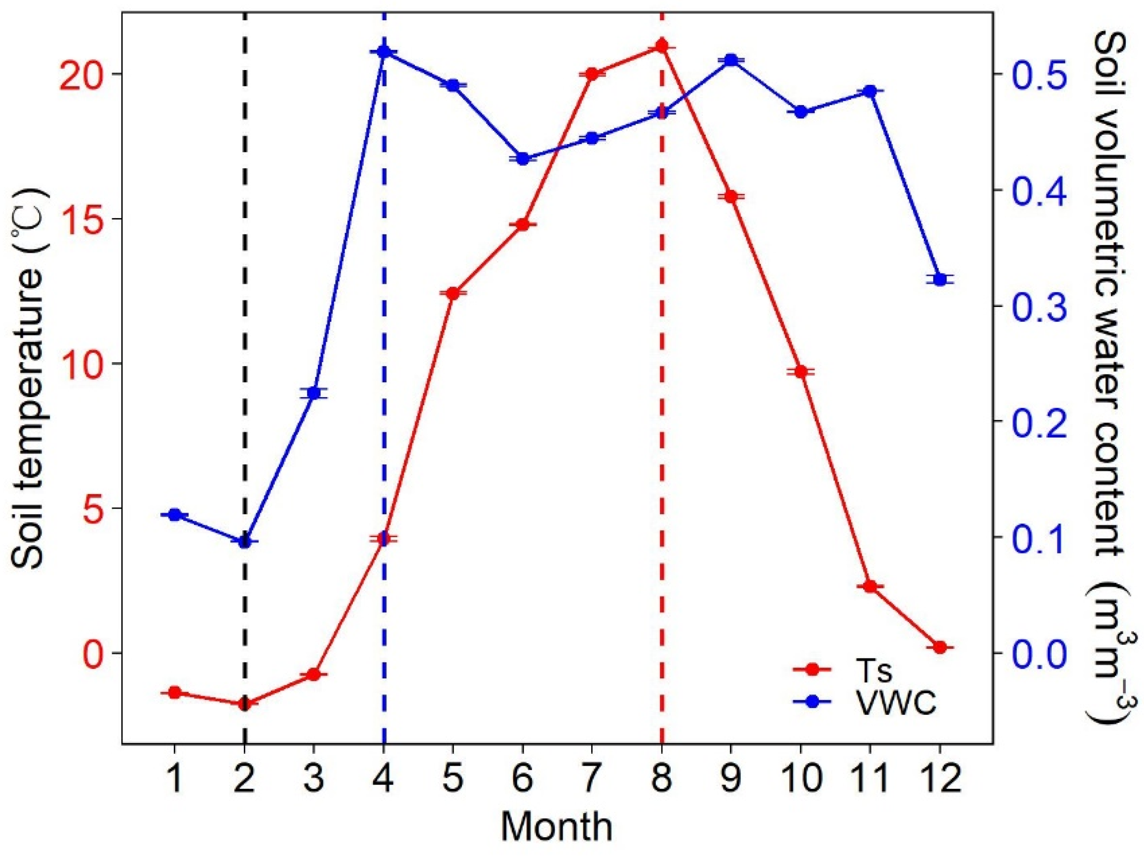
3.1. Environmental Factors

The Ts shows a clear unimodal pattern in the range of −1.8−21.0 °C, with the lowest values occurring in January and February and the highest in July and August (Figure 2). Both Ts and the VWC respond to seasonal climate changes, as indicated by the closely aligned valley values of both variables. The VWC exhibits a bimodal trend in the range of 0.10−0.52 m³ m⁻³, reaching its first peak in April and May and a second peak in the fall months (Figure 2).

3.2. Diurnal Variation Patterns in N₂O Flux and Optimal Sampling Time

Figure 3 illustrates the daily patterns of N₂O flux across different months of the year. A clear single-peak trend is observed in January, February, March, June, July, and October. In contrast, April, November, and December show a more stable pattern without distinct peaks or troughs, while May, August, and September exhibit multiple fluctuations. The flux typically peaks during the day and dips at night. Although nighttime fluxes are generally low, they occasionally surpass the daily average in March, April, November, and December. The times when the flux is closest to the daily mean differ by month. February, October, and December tend to have these moments in the morning (6:00−11:00), whereas January, June, and July see them in the afternoon (12:00−17:00). April and September align with the early night period (18:00−23:00), and March, May, and November show these times in the latter half of the night (0:00−5:00). When focusing solely on daytime data, only February, October, and December have their closest mean moments in the morning, while the other nine months are consistently in the afternoon, particularly from 12:00 to 16:00. Peak flux moments predominantly occur in the morning across most months, from May to November. The peak time occurs at 11:00 during May, July, August, September, and November. January and February deviate to the afternoon, and March, April, and December transition to the early night period. The trough moments display a varied distribution: February, March, April, and December have them in the morning, May, August, and September in the afternoon, and January, June, and October in the early night period. July and November, on the other hand, experience trough moments in the latter half of the night. Intermonthly variability in daily fluctuations is evident, with ranges extending from 0.00056−0.0063 nmol m⁻² s⁻¹ in January to 0.30−0.56 nmol m⁻² s⁻¹ in March, indicating the most significant fluctuations in March and the least in January (Figure 3).

Using the results of the Kruskal–Wallis and Wilcoxon tests at an annual scale (see

Table 1. The differences between daily averages and daytime or nighttime N₂O fluxes and between hourly N₂O flux and its corresponding daily average using the Kruskal–Wallis and Wilcoxon tests at the annual scale. Asterisks denote statistical significance levels: ns for p ≥ 0.05; * for p < 0.05; ** for p < 0.01; **** for p < 0.0001.

Scale	Kruskal–Wallis		Wilcoxon
	p-Value	Significance	Pairwise Comparison	Significance
Annual	<0.0001	****	Daytime vs. Full-day	****
			Nighttime vs. Full-day	****
Annual	<0.0001	****	1, 2, 3, 5, 13, 14, 15, 17, 22, 23 vs. 0–23	ns
			0, 4, 6, 16, 19, 20, 21 vs. 0–23	*
			7, 18 vs. 0–23	**
			8, 9, 10, 11, 12 vs. 0–23	****

), a highly significant difference (p < 0.0001) was identified between the daily average N₂O fluxes and those during the daytime or nighttime, observed consistently throughout the year. Further monthly analysis (

Table 2. The differences between daily averages (full-day) and daytime or nighttime N₂O fluxes using the Kruskal–Wallis and Wilcoxon tests at the monthly scale. Asterisks denote statistical significance levels: ns for p ≥ 0.05; ** for p < 0.01; *** for p < 0.001; **** for p < 0.0001.

Scale	Month	Kruskal–Wallis		Wilcoxon
		p-Value	Significance	Pairwise Comparison	Significance
Monthly	January, March and October	<0.0001	****	Daytime vs. Full-day	***
				Nighttime vs. Full-day	***
Monthly	February	0.0065	**	Daytime vs. Full-day	ns
				Nighttime vs. Full-day	ns
Monthly	April	0.9	ns
Monthly	May	<0.0001	****	Daytime vs. Full-day	****
				Nighttime vs. Full-day	***
Monthly	June, July and August	<0.0001	****	Daytime vs. Full-day	****
				Nighttime vs. Full-day	****
Monthly	September	<0.0001	****	Daytime vs. Full-day	**
				Nighttime vs. Full-day	**
Monthly	November	0.4	ns
Monthly	December	0.33	ns

) revealed similar significant differences in eight months, including January, March, May, June, July, August, September, and October. This not only reinforces the annual findings but also highlights a discernible pattern of seasonal variation in N₂O emissions, with the majority of significant differences occurring during the growing season from May to October. In contrast, no significant differences were observed in the non-growing season months (February, April, November, and December), except for January and March, which were influenced by freezing and thawing phenomena. The analysis from Table 1 indicates significant diurnal variations in N₂O fluxes, emphasizing the importance of considering these variations when measuring N₂O fluxes, as certain times of the day may disproportionately affect total emissions. Specifically, the deviation of N₂O fluxes from the daily mean was particularly significant between 8:00 and 12:00. In contrast, the fluxes observed at 1:00, 2:00, 3:00, 5:00, 13:00, 14:00, 15:00, 17:00, 22:00, and 23:00 were more stable and closer to the daily mean. Additionally, the flux values during the daytime hours of 13:00, 14:00, 15:00, and 17:00 were close to the daily mean, making these times ideal for monitoring N₂O fluxes. These findings are crucial for refining N₂O flux monitoring strategies and improving the accuracy of daily emissions estimation.

Figure 4 illustrates the cumulative monthly N₂O flux values at different sampling times (13:00, 14:00, 15:00, and 17:00) compared to those calculated from daily averages. Significant differences (p < 0.05) were observed at February 14:00 and 15:00; May 14:00, 15:00, and 17:00; July 13:00; and August 14:00. More pronounced differences (p < 0.01) were noted in January 13:00, March 17:00, August 15:00, and September 17:00. A very highly significant difference (p < 0.001) was found in September 15:00, and an extremely significant difference (p < 0.0001) was recorded in August 17:00. However, these differences were not significant in most cases, which suggests that afternoon hours, particularly 14:00, are optimal for N₂O flux observation sampling. These findings are crucial for refining N₂O flux monitoring strategies and improving sampling efficiency.

3.3. Correlation Between N₂O Flux and Environmental Factors

As shown in

Table 3. Correlation analysis of monthly soil N₂O flux with Ts and VWC (Pearson correlation coefficient and significance) and the temperature sensitivity (Q₁₀) of soil N₂O flux. Asterisks denote statistical significance levels: ns for p ≥ 0.05; * for p < 0.05; *** for p < 0.001; **** for p < 0.0001.

Month	1	2	3	4	5	6	7	8	9	10	11	12
r(N2O, Ts)	0.067	0.616	0.67	−0.393	0.108	0.207	−0.14	0.059	0.048	0.067	−0.434	0.135
p(N2O, Ts)	*	****	****	****	***	****	****	*	ns	*	****	****
r(N2O, VWC)	0.073	0.637	0.36	0.511	−0.176	0.228	0.057	0.125	0.148	−0.101	−0.153	−0.053
p(N2O, VWC)	*	****	****	****	****	****	*	****	****	***	****	ns
Q10	241.6	4 × 1013	1× 107	1 × 10−2	1.8	7.2	0.4	1.9	1.3	2.3	2 × 10−5	220.7

, soil N₂O fluxes were significantly correlated with Ts and VWC, except for the Ts in September and the VWC in December. A negative correlation with Ts was observed in April, July, and November, while other months showed a positive correlation. Similarly, soil N₂O fluxes were negatively correlated with soil VWC in May, October, November, and December but positively correlated in other months. Notably, Q₁₀ values were particularly high in January, February, March, and December, indicating heightened sensitivity of N₂O fluxes to temperature changes, whereas April and November exhibited lower Q₁₀ values. During the growing season (May–October), Q₁₀ values ranged from 0.4 to 7.2, with an average of 2.5. These findings provide critical insights into the seasonal dynamics and drivers of soil N₂O emissions.

The data in

Table 4. Optimal monthly soil N₂O flux estimated using Ts and VWC via stepwise regression. Asterisks denote statistical significance levels: ns p ≥ 0.05; ** p < 0.01; *** p < 0.001; **** p < 0.0001.

Month	Fitted Equation	R2	F	p
1	N2O flux = 0.003 + 0.027VWC	0.005	2.814	ns
2	N2O flux = −0.432 **** + 0.008Ts + 6.008VWC ****	0.406	410.5	****
3	N2O flux = 0.867 **** + 0.364Ts **** − 1.036VWC ****	0.53	790.2	****
4	N2O flux = −0.289 **** + 0.697VWC ****	0.261	230.4	****
5	N2O flux = 0.06 **** − 0.093VWC ****	0.031	18.4	****
6	N2O flux = −0.04 **** + 0.004Ts **** + 0.08VWC ****	0.075	56.5	****
7	N2O flux = 0.085 **** − 0.003Ts **** + 0.008VWC	0.02	13.8	****
8	N2O flux = −0.03 ** + 0.001Ts **** + 0.085VWC ****	0.031	21.8	****
9	N2O flux = 0.003 + 0.055VWC ****	0.022	15.8	****
10	N2O flux = 0.049 **** − 0.082VWC **	0.011	7.4	***
11	N2O flux = 0.113 **** − 0.006Ts **** − 0.202VWC ****	0.248	127.6	****
12	N2O flux = 0.312 **** + 0.173Ts **** − 0.753VWC ****	0.176	100.9	****

show that soil N₂O flux is influenced differently by Ts and VWC across months. Unlike January, most months exhibit statistically significant results (p < 0.05). February and March have the best model fits, indicating an effective explanation of N₂O flux variability, while fits are moderate for April, November, and December and lower for May through October. VWC significantly affects N₂O flux in all months except January and July, with positive correlations in February, April, June, August, and September and negative correlations in March, May, October, November, and December. Ts correlate positively with N₂O flux in March, June, August, and December and negatively in July and November. These findings reveal a complex interaction between soil N₂O lux and environmental factors that varies by month.

4. Discussion

4.1. Seasonal and Diurnal Patterns of N₂O Fluxes

The study revealed significant seasonal fluctuations in N₂O fluxes, with the most pronounced variability observed in March and relative stability in January, ranging from 0.00056 to 0.56 nmol m⁻² s⁻¹. This pattern aligns with findings from a German spruce forest, where freeze–thaw periods accounted for 87%–88% of annual N₂O emissions [37]. This is primarily due to dramatic changes in microbial activity and substrate availability during freeze–thaw cycles. Furthermore, increased freeze–thaw frequency under climate change may exacerbate seasonal N₂O emission variability [19,38], underscoring the importance of investigating freeze–thaw impacts on greenhouse gas emissions in a warming climate. In subtropical ecosystems, the highest N₂O emissions were observed during summer [39], consistent with another peak period for elevated emissions in this study, aside from the freeze–thaw periods. These results are also consistent with findings from a typical grassland ecosystem in Inner Mongolia, where peak emissions occurred during the growing season and spring freeze–thaw cycles, with minimal emissions during non-growing seasons [40]. Importantly, to mitigate N₂O emissions, nitrogen fertilizer application should avoid emission-sensitive periods, particularly during spring thaw and post-rainfall intervals with significant soil moisture fluctuations.

Diurnal variations in N₂O fluxes were observed, consistent with previous studies [12,13,14,15,39,41]. Notably, an unimodal pattern was more pronounced during high-emission periods, while no clear diurnal pattern was observed during low-emission periods, contrasting with findings from temperate agricultural ecosystems [9]. Diurnal patterns exhibited significant monthly variations, with higher daytime emissions during the growing season, consistent with most studies [5,12,13,38]. In winter (March, April, November, and December), higher nighttime emissions were likely linked to freeze–thaw cycles and limited soil nitrogen availability [19]. These findings align with previous research, indicating that diurnal N₂O emissions are regulated by both environmental factors and biological processes [4]. Significant differences between daytime and nighttime fluxes and daily averages highlight the importance of considering diurnal variations in monitoring strategies, as certain periods may disproportionately influence total emissions.

4.2. Optimal Sampling Time for N₂O Fluxes

N₂O fluxes exhibited significant diurnal variations, with peak emissions during the growing season (May–October) typically occurring at 11:00. However, many previous studies focused on sampling between 9:00 and 11:00 [42,43,44,45,46], potentially leading to overestimation of soil N₂O fluxes. This study recommends avoiding 11:00 to estimate daily average N₂O fluxes. Peak emissions in January and February occurred in the afternoon, while March, April, and December showed peaks in the early evening. Troughs were observed in the morning for February, March, April, and December; in the afternoon for May, August, and September; and at night for January, June, July, October, and November. These findings provide critical insights for improving N₂O flux monitoring and emission estimation accuracy. Fluxes at 13:00, 14:00, 15:00, and 17:00 were closest to daily averages, with 14:00 being the optimal sampling time. This finding is crucial for enhancing monitoring efficiency and accuracy, enabling more targeted sampling. Similar observations have been reported [11], likely because emissions during these periods fall between nighttime and daytime peaks, better representing daily averages.

4.3. Environmental Factors Influencing N₂O Emissions and Their Correlations

Seasonal variations in N₂O emissions were primarily driven by changes in soil temperature and moisture [47]. Ts followed an unimodal pattern with higher summer and lower winter values. In contrast, VWC demonstrated a bimodal trend during the periods of snowmelt and rainfall, indicating its sensitivity to seasonal climate variations. The synchronized troughs in soil temperature and VWC suggest a degree of co-variation in their seasonal dynamics. The relationship between N₂O fluxes and Ts and VWC varied significantly across seasons. In January, the relationship was statistically insignificant, consistent with findings that frozen forest soils can produce N₂O through denitrification under anaerobic conditions, unaffected by low temperatures, and maintain net nitrogen mineralization and nitrification [48,49,50]. The best-fit relationships between N₂O fluxes and Ts and VWC were observed in February and March, indicating strong regulatory effects during these months. The relationship between Ts and N₂O fluxes showed both positive and negative correlations across months, reflecting the complex effects of temperature on microbial activity and substrate availability [22,51]. Negative correlations in July and November may result from VWC stress induced by high temperatures, suppressing microbial activity. Additionally, high Q₁₀ values in January, February, March, and December suggest greater temperature sensitivity of N₂O fluxes during these months, likely due to soil structure disruption and substrate release during freeze–thaw cycles. During the growing season (May–October), Q₁₀ values ranged from 0.4 to 7.2, averaging 2.5, consistent with previous studies [22,52,53,54]. Research in UK Sitka spruce plantations demonstrated an exponential temperature response (Q₁₀ = 3.3); therefore, the N₂O flux peaked in summer [55]. Except for January and July, VWC significantly influenced N₂O fluxes, highlighting the importance of soil VWC in regulating emissions. However, the relationship is complex, as moderate VWC levels favor denitrification and N₂O production [9,10,17,56], while excessive VWC may create anaerobic conditions, inhibiting microbial activity [4,27]. For example, during the growing season, high VWC and limited oxygen availability may enhance N₂O reduction to N₂, weakening N₂O emissions with increasing soil moisture [27,57]. Conversely, elevated winter fluxes in Italy’s Monte Morello mixed-conifer stands due to moist, litter-rich conditions [58], while eastern white pine forests in Ontario transition from functioning as N₂O sinks under dry conditions (soil moisture <15%) to emission sources at higher moisture levels [59]. Recent studies have demonstrated that snowpack dynamics and vegetation structure significantly regulate soil moisture patterns and N₂O flux variations, underscoring the need to better understand understory transpiration processes, pioneer tree water competition dynamics, and snow-influenced microbial interactions [60]. The coupling of Ts and VWC plays a critical role in regulating N₂O emissions, as their synergistic effects may influence microbial community structure and function, further modulating N₂O production and release [2]. By revealing key climate change impacts on soil ecosystems, these findings directly support creating dual-parameter (temperature–moisture) monitoring systems to predict and mitigate high-emission events. While the identified drivers provide meaningful insights, we acknowledge the need to explore more sophisticated approaches (e.g., machine learning or nonlinear models incorporating interaction terms) in future studies to enhance explanatory power.

5. Conclusions

Through year-round continuous monitoring of soil N₂O flux in a temperate mixed forest ecosystem, this study revealed significant seasonal and diurnal variation patterns. The most pronounced fluctuations were observed in March, while relatively stable conditions prevailed in January. Diurnal variation patterns showed significant monthly differences, with N₂O emission peaks typically occurring at 11:00 during the growing season, while higher nighttime emissions were observed in winter. The optimal sampling time was identified as 14:00, as measurements taken between 13:00 and 17:00 closely approximated the daily average values. We recommend conducting monitoring during this time window to improve data representativeness. Ts and VWC exhibited significant seasonal differences in their effects on N₂O emissions, with the best-fitting results observed in February and March indicating strong regulatory effects of these factors on N₂O emissions. The Q₁₀ values during the growing season ranged from 0.4 to 7.2, with an average of 2.5, demonstrating the high sensitivity of N₂O fluxes to temperature changes. The influence of soil VWC on N₂O emissions was more complex: moderately moist conditions favored denitrification processes, while excessive VWC could inhibit microbial activity. These findings highlight the importance of considering both temporal variability and environmental factors when monitoring and estimating N₂O fluxes. This comprehensive approach is crucial for understanding and mitigating the impact of N₂O emissions from forest ecosystems on global warming.

References

1. Maucieri, C.; Barbera, A.C.; Vymazal, J.; Borin, M. A review on the main affecting factors of greenhouse gases emission in constructed wetlands. Agric. For. Meteorol. 2017, 236, 175–193. [Google Scholar] [CrossRef]
2. Tian, H.; Xu, R.; Canadell, J.G.; Thompson, R.L.; Yao, Y. A comprehensive quantification of global nitrous oxide sources and sinks. Nature 2020, 586, 248–256. [Google Scholar] [CrossRef] [PubMed]
3. IPCC. 2006 IPCC Guidelines for National Greenhouse Gas Inventories; Prepared by the National Greenhouse Gas Inventories Programme; Eggleston, H.S., Buendia, L., Miwa, K., Ngara, T., Tanabe, K., Eds.; IGES: Hayama, Japan, 2006. [Google Scholar]
4. Smith, P.; Martino, D.; Cai, Z.; Gwary, D.; Smith, J. Greenhouse gas mitigation in agriculture. Philos. Trans. R. Soc. B-Biol. Sci. 2008, 363, 789–813. [Google Scholar] [CrossRef] [PubMed]
5. Alves, B.J.R.; Smith, K.A.; Flores, R.A.; Cardoso, A.S.; Oliveira, W.R.D.; Jantalia, C.P.; Urquiaga, S.; Boddey, R.M. Selection of the most suitable sampling time for static chambers for the estimation of daily mean N2O flux from soils. Soil Biol. Biochem. 2012, 46, 129–135. [Google Scholar] [CrossRef]
6. Kurganova, I.; Teepe, R.; Loftfield, N. Influence of freeze-thaw events on carbon dioxide emission from soils at different moisture and land use. Carbon Balance Manag. 2007, 2, 2. [Google Scholar] [CrossRef]
7. Wang, C.; Han, Y.; Chen, J.; Wang, X.; Zhang, Q.; Bond-Lamberty, B. Seasonality of soil CO2 efflux in a temperate forest: Biophysical effects of snowpack and spring freeze–thaw cycles. Agric. For. Meteorol. 2013, 177, 83–92. [Google Scholar] [CrossRef]
8. Wu, G.; Chen, X.M.; Ling, J.; Li, F.; Zhou, S.L. Effects of soil warming and increased precipitation on greenhouse gas fluxes in spring maize seasons in the North China Plain. Sci. Total Environ. 2020, 734, 139269. [Google Scholar] [CrossRef]
9. Clar, J.T.F.; Anex, R.P. Flux intensity and diurnal variability of soil N2O emissions in a highly fertilized cropping system. Soil Sci. Soc. Am. J. 2020, 84, 1983–1994. [Google Scholar] [CrossRef]
10. Keane, J.B.; Morrison, R.; Mcnamara, N.P.; Ineson, P. Real-time monitoring of greenhouse gas emissions with tall chambers reveals diurnal N2O variation and increased emissions of CO2 and N2O from Miscanthus following compost addition. Glob. Change Biol. Bioenergy 2019, 11, 1456–1470. [Google Scholar] [CrossRef]
11. Xu, X.; Fu, G.; Zou, X.; Ge, C.; Zhao, Y. Diurnal variations of carbon dioxide, methane, and nitrous oxide fluxes from invasive Spartina alterniflora dominated coastal wetland in northern Jiangsu Province. Acta Oceanol. Sin. 2017, 36, 105–113. [Google Scholar] [CrossRef]
12. Wu, Y.F.; Whitaker, J.; Toet, S.; Bradley, A.; Davies, C.A.; Mcnamara, N.P. Diurnal variability in soil nitrous oxide emissions is a widespread phenomenon. Glob. Change Biol. 2021, 27, 4950–4966. [Google Scholar] [CrossRef] [PubMed]
13. Yang, H.; Liu, S.; Li, Y.; Xu, H. Diurnal variations and gap effects of soil CO2, N2O and CH4 fluxes in a typical tropical montane rainforest in Hainan Island, China. Ecol. Res. 2018, 33, 379–392. [Google Scholar] [CrossRef]
14. Xiao, D.M.; Wang, M.; Wang, Y.S.; Ji, L.Z.; Han, S.J. Fluxes of soil carbon dioxide, nitrous oxide and firedamp in broadleaved/Korean pine forest. J. For. Res. 2004, 15, 107–112. [Google Scholar]
15. Richardson, A.D.; Hollinger, D.Y.; Shoemaker, J.K.; Hughes, H.; Davidson, E.A. Six years of ecosystem-atmosphere greenhouse gas fluxes measured in a sub-boreal forest. Sci. Data 2019, 6, 117. [Google Scholar] [CrossRef]
16. Zhang, L.H.; Song, L.P.; Zhang, L.W.; Shao, H.B. Diurnal dynamics of CH4, CO2 and N2O fluxes in the saline-alkaline soils of the Yellow River Delta, China. Plant Biosyst. 2015, 149, 797–805. [Google Scholar] [CrossRef]
17. Zona, D.; Janssens, I.A.; Gioli, B.; Jungkunst, H.F. N2O fluxes of a bio-energy poplar plantation during a two years rotation period. Glob. Change Biol. Bioenergy 2013, 5, 536–547. [Google Scholar] [CrossRef]
18. Taneva, L.; Gonzalez-Meler, M.A. Distinct patterns in the diurnal and seasonal variability in four components of soil respiration in a temperate forest under free-air CO2 enrichment. Biogeosciences 2011, 8, 3077–3092. [Google Scholar] [CrossRef]
19. Shurpali, N.J.; Rannik, Ü.; Jokinen, S.; Lind, S.; Biasi, C.; Mammarella, I.; Peltala, O.; Pihlatie, M.; Hyvönen, N.; Räty, M.; et al. Neglecting diurnal variations leads to uncertainties in terrestrial nitrous oxide emissions. Sci. Rep. 2016, 6, 25739. [Google Scholar] [CrossRef]
20. Hall, M.K.D.; Winters, A.J.; Rogers, G.S. Variations in the Diurnal Flux of Greenhouse Gases from Soil and Optimizing the Sampling Protocol for Closed Static Chambers. Commun. Soil Sci. Plant Anal. 2014, 45, 2970–2978. [Google Scholar] [CrossRef]
21. Savage, K.; Phillips, R.; Davidson, E. High temporal frequency measurements of greenhouse gas emissions from soils. Biogeosciences 2014, 11, 2709–2720. [Google Scholar] [CrossRef]
22. Butterbach-Bahl, K.; Baggs, E.M.; Dannenmann, M.; Kiese, R.; Zechmeister-Boltenstern, S. Nitrous oxide emissions from soils: How well do we understand the processes and their controls? Philos. Trans. R. Soc. B-Biol. Sci. 2013, 368, 20130122. [Google Scholar] [CrossRef] [PubMed]
23. Zang, H.; Blagodatskaya, E.; Wen, Y.; Shi, L.; Cheng, F.; Chen, H.; Zhao, B.; Zhang, F.; Fan, M.; Kuzyakov, Y. Temperature sensitivity of soil organic matter mineralization decreases with long-term N fertilization: Evidence from four Q10 estimation approaches. Land Degrad. Dev. 2020, 31, 683–693. [Google Scholar] [CrossRef]
24. Tu, C.; Li, F.D. Responses of greenhouse gas fluxes to experimental warming in wheat season under conventional tillage and no-tillage fields. J. Environ. Sci. 2017, 54, 314–327. [Google Scholar] [CrossRef]
25. Blankinship, J.C.; Brown, J.R.; Dijkstra, P.; Allwright, M.C.; Hungate, B.A. Response of terrestrial CH4 uptake to interactive changes in precipitation and temperature along a climatic gradient. Ecosystems 2010, 13, 1157–1170. [Google Scholar] [CrossRef]
26. Sponseller, R.A. Precipitation pulses and soil CO2 flux in a Sonoran Desert ecosystem. Glob. Change Biol. 2007, 13, 426–436. [Google Scholar] [CrossRef]
27. Wen, Y.; Zang, H.; Freeman, B.; Ma, Q.; Jones, D.L. Rye cover crop incorporation and high watertable mitigate greenhouse gas emissions in cultivated peatland. Land Degrad. Dev. 2019, 30, 1928–1938. [Google Scholar] [CrossRef]
28. Li, J.; Sang, C.; Yang, J.; Qu, L.; Xia, Z.; Sun, H.; Jiang, P.; Wang, X.; He, H.; Wang, C. Stoichiometric imbalance and microbial community regulate microbial elements use efficiencies under nitrogen addition. Soil Biol. Biochem. 2021, 156, 108207. [Google Scholar] [CrossRef]
29. Li, Z.; Cao, L.; Sun, F.; Ye, H.; Duan, Y.; Liu, Z. Study on the Impact of Climate Change on Water Cycle Processes in Cold Mountainous Areas—A Case Study of Water Towers in Northeastern China. Water 2025, 17, 969. [Google Scholar] [CrossRef]
30. Chen, Z.; Setälä, H.; Geng, S.; Han, S.; Wang, S.; Dai, G.; Zhang, J. Nitrogen addition impacts on the emissions of greenhouse gases depending on the forest type: A case study in Changbai Mountain, Northeast China. J. Soils Sediments 2017, 17, 23–34. [Google Scholar] [CrossRef]
31. IUSS Working Group WRB. World Reference Base for Soil Resources. International Soil Classification System for Naming Soils and Creating Legends for Soil Maps, 4th ed.; International Union of Soil Sciences (IUSS): Vienna, Austria, 2022. [Google Scholar]
32. Guo, C.; Zhang, L.; Li, S.; Chen, Y. Freeze-Thaw Events Change Soil Greenhouse Gas Fluxes Through Modifying Soil Carbon and Nitrogen Cycling Processes in a Temperate Forest in Northeastern China. Forests 2024, 15, 2082. [Google Scholar] [CrossRef]
33. Guo, C.; Zhang, L.; Li, S.; Li, Q.; Dai, G. Comparison of Soil Greenhouse Gas Fluxes during the Spring Freeze–Thaw Period and the Growing Season in a Temperate Broadleaved Korean Pine Forest, Changbai Mountains, China. Forests 2020, 11, 1135. [Google Scholar] [CrossRef]
34. Liu, H.; Zheng, X.; Li, Y.; Yu, J.; Zhang, Y. Soil moisture determines nitrous oxide emission and uptake. Sci. Total Environ. 2022, 822, 153566. [Google Scholar] [CrossRef] [PubMed]
35. Zhou, Y.; Hagedorn, F.; Zhou, C.; Jiang, X.; Wang, X.; Li, M. Experimental warming of a mountain tundra increases soil CO2 effluxes and enhances CH4 and N2O uptake at Changbai Mountain, China. Sci. Rep. 2016, 6, 21108. [Google Scholar] [CrossRef] [PubMed]
36. R Core Team. R: A Language and Environment for Statistical Computing. R Foundation for Statistical Computing: Vienna, Austria, 2023. Available online: https://www.R-project.org/ (accessed on 28 April 2025).
37. Luo, G.; Brüggemann, N.; Wolf, B.; Gasche, R.; Grote, R.; Butterbach-Bahl, K.; Cellier, P. Decadal variability of soil CO2, NO, N2O, and CH4 fluxes at the Hoglwald forest, Germany. Biogeosciences 2012, 9, 1741–1763. [Google Scholar] [CrossRef]
38. Du, R.; Lu, D.R.; Wang, G.C. Diurnal, seasonal, and inter-annual variations of N2O fluxes from native semi-arid grassland soils of inner Mongolia. Soil Biol. Biochem. 2006, 38, 3474–3482. [Google Scholar] [CrossRef]
39. Tsai, C.P.; Huang, C.M.; Yuan, C.S.; Yang, L. Seasonal and diurnal variations of greenhouse gas emissions from a saline mangrove constructed wetland by using an in situ continuous GHG monitoring system. Environ. Sci. Pollut. Res. 2020, 27, 15824–15834. [Google Scholar] [CrossRef]
40. Wolf, B.; Zheng, X.; Brüggemann, N.; Chen, W.; Dannenmann, M.; Han, X.; Sutton, M.; Wu, H.; Yao, Z.; Butterbach-Bahl, K. Grazing-induced reduction of natural nitrous oxide release from continental steppe. Nature 2010, 464, 881–884. [Google Scholar] [CrossRef]
41. Barba, J.; Poyatos, R.; Vargas, R. Automated measurements of greenhouse gases fluxes from tree stems and soils: Magnitudes, patterns and drivers. Sci. Rep. 2019, 9, 4005. [Google Scholar] [CrossRef]
42. Zheng, Z.M.; Yu, G.R.; Sun, X.M.; Li, S.G.; Wang, Y.S.; Wang, Y.H.; Fu, Y.L.; Wang, Q.F. Spatio-Temporal Variability of Soil Respiration of Forest Ecosystems in China: Influencing Factors and Evaluation Model. J. Environ. Manag. 2010, 46, 633–642. [Google Scholar] [CrossRef]
43. Liu, J.; Chen, H.; Yang, X.; Gong, Y.; Zheng, X.; Fan, M.; Kuzyakov, Y. Annual methane uptake from different land uses in an agro-pastoral ecotone of northern China. Agric. For. Meteorol. 2017, 236, 67–77. [Google Scholar] [CrossRef]
44. Yang, X.M.; Chen, H.Q.; Gong, Y.S.; Zheng, X.H.; Fan, M.S. Nitrous oxide emissions from an agro-pastoral ecotone of northern China depending on land uses. Agric. Ecosyst. Environ. 2015, 213, 241–251. [Google Scholar] [CrossRef]
45. Gasche, R.; Papen, H. A 3-year continuous record of nitrogen trace gas fluxes from untreated and limed soil of a N-saturated spruce and beech forest ecosystem in Germany: 2.: NO and NO2 fluxes. J. Geophys. Res.-Atmos. 1999, 104, 18505–18520. [Google Scholar] [CrossRef]
46. Su, C.X.; Zhu, W.X.; Kang, R.H.; Quan, Z.; Liu, D.W.; Huan, W.T.; Shi, Y.; Chen, X.; Fang, Y.T. Interannual and seasonal variabilities in soil NO fluxes from a rainfed maize field in the Northeast China. Environ. Pollut. 2021, 286, 117312. [Google Scholar] [CrossRef] [PubMed]
47. Hu, Y.; Chang, X.; Lin, X.; Wang, Y.; Wang, S.; Duan, J.; Zhang, Z.; Yang, X.; Luo, C.; Xu, G.; et al. Effects of warming and grazing on N2O fluxes in an alpine meadow ecosystem on the Tibetan plateau. Soil Biol. Biochem. 2010, 42, 944–952. [Google Scholar] [CrossRef]
48. Öquist, M.G.; Nilsson, M.; Sörensson, F.; Kasimir-Klemedtsson, Å.; Persson, T.; Weslien, P.; Klemedtsson, L. Nitrous oxide production in a forest soil at low temperatures—Processes and environmental controls. FEMS Microbiol. Ecol. 2004, 49, 371–378. [Google Scholar] [CrossRef]
49. Goldberg, S.D.; Borken, W.; Gebauer, G. N2O emission in a Norway spruce forest due to soil frost: Concentration and isotope profiles shed a new light on an old story. Biogeochemistry 2010, 97, 21–30. [Google Scholar] [CrossRef]
50. Peng, B.; Sun, J.; Liu, J.; Dai, W.; Sun, L.; Pei, G.; Gao, D.; Wang, C.; Jiang, P.; Bai, E. N2O emission from a temperate forest soil during the freeze-thaw period: A mesocosm study. Sci. Total Environ. 2019, 648, 350–357. [Google Scholar] [CrossRef]
51. Smith, K.A. Changing views of nitrous oxide emissions from agricultural soil: Key controlling processes and assessment at different spatial scales. Eur. J. Soil Sci. 2017, 68, 137–155. [Google Scholar] [CrossRef]
52. Yu, H.M.; Duan, Y.H.; Mulder, J.; Dörsch, P.; Zhu, W.X.; Xu, R.; Huang, K.; Zheng, Z.T.; Kang, R.H.; Wang, C.; et al. Universal temperature sensitivity of denitrification nitrogen losses in forest soils. Nat. Clim. Change 2023, 13, 726–734. [Google Scholar] [CrossRef]
53. Sitaula, B.K.; Bakken, L.R. Nitrous oxide release from spruce forest soil: Relationships with nitrification, methane uptake, temperature, moisture and fertilization. Soil Biol. Biochem. 1993, 25, 1415–1421. [Google Scholar] [CrossRef]
54. Brumme, R. Mechanisms of carbon and nutrient release and retention in beech forest gaps III. Environmental regulation of soil respiration and nitrous oxide emissions along a microclimatic gradient. Plant Soil 1995, 168, 593–600. [Google Scholar] [CrossRef]
55. Ball, T.; Smith, K.A.; Moncrieff, J.B. Effect of stand age on greenhouse gas fluxes from a Sitka spruce Picea sitchensis (Bong.) Carr. chronosequence on a peaty gley soil. Glob. Change Biol. 2007, 13, 2128–2142. [Google Scholar] [CrossRef]
56. McCalley, C.K.; Woodcroft, B.J.; Hodgkins, S.B.; Wehr, R.A.; Kim, E.H.; Mondav, R.; Crill, P.M.; Chanton, J.P.; Rich, V.I.; Tyson, G.W.; et al. Methane dynamics regulated by microbial community response to permafrost thaw. Nature 2014, 514, 478–481. [Google Scholar] [CrossRef] [PubMed]
57. Davidson, E.A.; Vitousek, P.M.; Matson, P.A.; Riley, R.; García-Méndez, G.; Maass, J.M. Soil emissions of nitric oxide in a seasonally dry tropical forest of México. J. Geophys. Res. 1991, 96, 439–445. [Google Scholar] [CrossRef]
58. Mazza, G.; Agnelli, A.E.; Lagomarsino, A. The Effect of Tree Species Composition on Soil C and N Pools and Greenhouse Gas Fluxes in a Mediterranean Reforestation. J. Soil Sci. Plant Nutr. 2021, 21, 1339–1352. [Google Scholar] [CrossRef]
59. Peichl, M.; Arain, M.A.; Ullah, S.; Moore, T.R. Carbon dioxide, methane, and nitrous oxide exchanges in an age-sequence of temperate pine forests. Glob. Change Biol. 2009, 16, 2198–2212. [Google Scholar] [CrossRef]
60. Murariu, G.; Dinca, L.; Tudose, N.; Crisan, V.; Georgescu, L.; Munteanu, D.; Dragu, M.D.; Rosu, B.; Mocanu, G.D. Structural Characteristics of the Main Resinous Stands from Southern Carpathians, Romania. Forests 2021, 12, 1029. [Google Scholar] [CrossRef]
Figure 1. Spatial distribution of the dynamic chambers (Chambers 1–8).
Forests 16 00766 g001
Figure 2. Variations in monthly soil temperature (Ts) and soil volumetric water content (VWC) at a 5 cm depth. The red dashed line indicates the peak value of Ts, the blue dashed line indicates the peak value of VWC, and the black dashed line indicates the valley values of Ts and VWC. Also, standard errors are shown as error bars. In future studies (data from 2019), seasonal snow cover (winter–spring) at the same site is expected to reach peak depths of 10 cm [33].
Forests 16 00766 g002
Figure 3. Monthly diurnal patterns of soil N2O fluxes for the entire year, with standard errors indicated as error bars: (a) January, (b) February, (c) March, (d) April, (e) May, (f) June, (g) July, (h) August, (i) September, (j) October, (k) November, (l) December. The horizontal dashed line represents the monthly daily average N2O flux value. The grey shaded area indicates daytime, from 6 to 17. The vertical dashed line indicates the hour closest to the daily average value, and the vertical dotted line shows the hour closest to the daily average value during daytime hours (6:00−17:00) if the closest hour falls within the nighttime period (18:00−5:00 the following day).
Forests 16 00766 g003
Figure 4. Monthly cumulative N2O flux for sampling times 13 (13:00), 14 (14:00), 15 (15:00), 17 (17:00), and daily average (the full day: 0−23 (0:00−23:00)): (a) January, February, March; (b) April, May, June; (c) July, August, September; (d) October, November, December. Asterisks denote significant differences (* for p < 0.05; ** for p < 0.01; *** for p < 0.001; **** for p < 0.0001) between hourly fluxes and their corresponding daily averages. Additionally, standard errors are shown as error bars.
Forests 16 00766 g004