Article

Improvement of 3D Green Volume Estimation Method for Individual Street Trees Based on TLS Data

Centre of Co-Innovation for Sustainable Forestry in Southern China, Nanjing Forestry University, Nanjing 210037, China
*
Author to whom correspondence should be addressed.
Forests 2025, 16(4), 690; https://doi.org/10.3390/f16040690
Submission received: 5 March 2025 / Revised: 12 April 2025 / Accepted: 15 April 2025 / Published: 16 April 2025
(This article belongs to the Section Urban Forestry)

Abstract

:
Vertical structure monitoring of urban vegetation provides data support for urban green space planning and ecological management, playing a significant role in promoting sustainable urban ecological development. Three-dimensional green volume (3DGV) is a comprehensive index used to characterize the ecological benefit of urban vegetation. As a critical component of urban vegetation, street trees play a key role in urban ecological benefits evaluation, and the quantitative estimation of their 3DGV serves as the foundation for this assessment. However, current methods for measuring 3DGV based on point cloud data often suffer from issues of overestimation or underestimation. To improve the accuracy of the 3DGV for urban street trees, this study proposed a novel approach that used convex hull coupling k-means clustering convex hulls. A new method based on terrestrial laser scanning (TLS) data was proposed, referred to as the Convex Hull Coupling Method (CHCM). This method divides the tree crown into two parts in the vertical direction according to the point cloud density, which better adapts to the lower density of the upper layer of TLS data and obtains a more accurate 3DGV of individual trees. To validate the effectiveness of the CHCM method, 30 sycamore (Platanus × acerifolia (Aiton) Willd.) plants were used as research objects. We used the CHCM and five traditional 3DGV calculation methods (frustum method, convex hull method, k-means clustering convex hulls, alpha-shape algorithm, and voxel-based method) to calculate the 3DGV of individual trees. Additionally, the 3DGV was predicted and analyzed using five fitting models. The results show the following: (1) Compared with the traditional methods, the CHCM improves the estimation accuracy of the 3DGV of individual trees and shows a high consistency in the data verification, which indicates that the CHCM method is stable and reliable, and (2) the fitting results R² of the five models were all above 0.75, with the exponential function model showing the best fitting accuracy (R2 = 0.89, RMSE = 74.85 m3). These results indicate that for TLS data, the CHCM can achieve more accurate 3DGV estimates for individual trees, outperforming traditional methods in both applicability and accuracy. The research results not only offer a novel technical approach for 3DGV calculation using TLS data but also establish a reliable quantitative foundation for the scientific assessment of the ecological benefits of urban street trees and green space planning.

1. Introduction

Urban vegetation is a critical component of the urban ecosystem, playing a significant role in environmental maintenance, biodiversity conservation, and urban landscaping [1]. In recent decades, numerous scholars have conducted extensive research on urban green volume, utilizing it as an index to assess the quality of the urban living environment [2,3,4]. People usually use two-dimensional greening indicators, such as the greening rate, green coverage rate, and per capita green area, to evaluate the basic greening status in a certain area [5,6]. However, these indicators can only describe the overall greening situation in a region from a two-dimensional perspective and fail to reflect the impact of vegetation on urban ecological environmental benefits and ecological functions from a three-dimensional spatial pattern. With the introduction of the concept of three-dimensional green volume (3DGV), research has gradually shifted from a two-dimensional plane to a three-dimensional space [7]. Three-dimensional green volume refers to the space volume occupied by the stems and leaves of all growing plants. It provides a more comprehensive understanding of the distribution rationality of urban vegetation and holds significant reference value for ecological evaluation and planning decisions related to urban vegetation [8,9,10]. However, accurately and efficiently estimating the 3DGV of urban vegetation remains an urgent technical challenge.
Three-dimensional green volume is a crucial factor in evaluating the growth of tree canopy. The canopy is an irregular, non-solid structure composed of gaps. Accurately measuring its 3DGV is challenging because it would require removing branches, which is not feasible without altering the canopy’s natural state [11]. The traditional method usually treats the tree canopy as a regular geometry, and fits the canopy shape according to the canopy width and canopy height parameters, to estimate the 3DGV [12,13]. However, the accuracy of this method is limited, as it overlooks variations in tree canopy shape and the spatial distribution of leaves, leading to significant errors in the estimation. With the rapid advancement of remote sensing technology, LiDAR scanning has become widely used in forestry surveys [14,15,16]. The calculation of 3DGV based on LiDAR point cloud data has become a key method for evaluating the ecological benefits of urban greening [17,18].
Methods for calculating 3DGV from point cloud data can generally be classified into two categories: One is the complete 3D reconstruction of the point cloud. These methods directly construct a complete 3D model of tree canopy using LiDAR point cloud data, typically employing geometric algorithms, such as the convex hull method [19] and the alpha-shape algorithm [20]. For instance, Li et al. [21] used backpack-style LiDAR to acquire 3D point cloud data and applied the convex hull method to calculate the 3DGV of individual tree canopies. The results showed that, compared to traditional methods, the maximum error of this approach was 33.70%, while the minimum error was 10.70%. Similarly, Korhonen et al. [22] used airborne laser scanning (ALS) data and applied the 3D convex hull method and the alpha-shape algorithm to estimate canopy volume, with results showing a strong correlation with field measurements. These methods typically focus on calculating the external shape of the tree crown and may not adequately account for the internal details, leading to less accurate assessments of the canopy’s internal structure. The other category is based on the concept of segmentation. This approach involves dividing the tree crown into multiple parts, calculating the volume of each par individually, and then combining them to obtain the total 3DGV of the tree, such as the frustum method and voxel-based method. For example, Wang [23] improved upon the frustum method by layering the tree crown and using a dynamically set α threshold in the α-shape algorithm to calculate the slice area, achieving precise computation of the canopy volume. Fernandez-Sarria et al. [24] used terrestrial laser scanning (TLS) data and applied the voxel-based method to extract the 3DGV of plane trees (R2 = 0.78), demonstrating the potential of TLS data in predicting the 3DGV of urban vegetation. Huang et al. [25] combined the voxel-based measurement method with a point cloud organized using an octree structure to propose a new 3DGV estimation model. Additionally, Wang et al. [26] applied the k-means clustering algorithm to segment the point cloud into multiple clusters, generating a detailed 3D description of vegetation canopy clusters. These methods effectively reduce the overestimation issue through segmentation and offer relative flexibility in computation. Overall, LiDAR point cloud data provide a reliable means for estimating 3DGV. Compared to traditional methods, this technology demonstrates higher applicability, especially in cases with complex tree canopy structures.
Street trees are an important part of urban vegetation, forming the structural framework and backbone of urban greening. They can connect the ecological corridor of the entire city in a series [27]. Street trees play an important role in reducing environmental pollution, improving the urban microclimate, purifying the air, reducing noise, slowing wind speed, and beautifying the urban environment [28]. At the same time, street trees embody the personality and cultural characteristics of a city and play an irreplaceable role in urban road greening. Due to their ornamental and aesthetic value, destructive methods are not suitable for studying the 3DGV of street trees. Therefore, the non-destructive measurement of street tree 3DGV is of great significance for the scientific evaluation of urban ecological function and environmental effect mechanism [29]. As the fundamental component unit of street trees, the quantitative description of individual trees’ 3DGV serves as the foundation for estimating the 3DGV of urban vegetation.
The sycamore (Platanus × acerifolia (Aiton) Willd.) is a world-renowned urban greening tree species. It is widely distributed in cities around the world for its rapid growth, aesthetically pleasing form, and strong adaptability [30]. Accurate estimation of the 3DGV of an individual sycamore tree is of significance for the vertical structure monitoring and greening management of street trees. Based on this, a new method for calculating the 3DGV of individual trees based on TLS data was proposed in this study. Based on existing methods, the convex hull coupling k-means clustering convex hulls method (referred to as the Convex Hull Coupling Method (CHCM)) was combined to verify the accuracy of the 3DGV calculation of sycamores as the research object. The purpose of this study is as follows: (1) to construct an optimized method for estimating 3DGV and to prove the reliability and accuracy of the CHCM by comparing it with other methods. (2) Different models were used to fit the 3DGV. The fitting effects of different models were evaluated and combined with actual data, and the best-fitting model was finally selected for prediction. This aims to provide a scientific basis and model support for the accurate estimation of the 3DGV of individual trees.

2. Materials and Methods
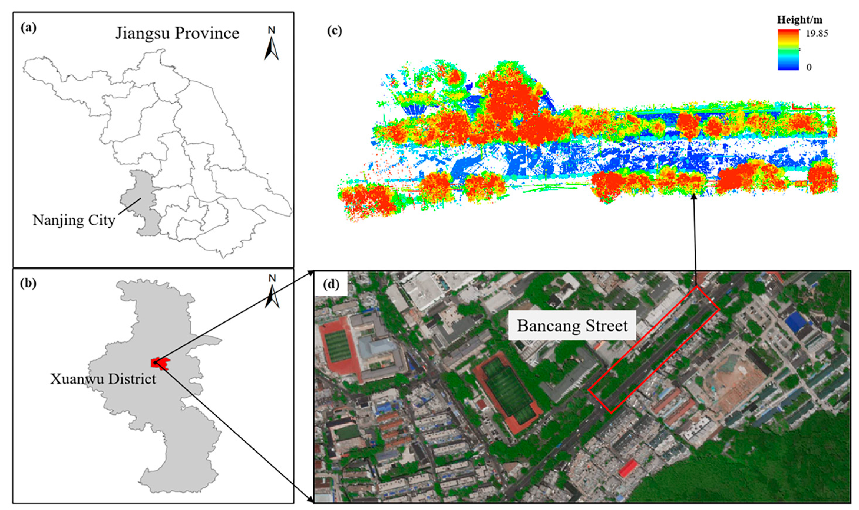
2.1. Study Area

The study area is located in Bancang Street, Xuanwu District, Nanjing City, Jiangsu Province, China (Figure 1). Nanjing (31°14′–32°37′ N, 118°22′–119°14′ E) is the capital city of Jiangsu Province and the political, economic, and cultural center of South China. The study area experiences a subtropical monsoon climate characterized by four distinct seasons and abundant rainfall. The average annual temperature is 15.4 °C, and the average annual precipitation is 1106 mm. The terrain predominantly consists of low mountains and gentle hills [31]. The primary street trees include sycamore, Ginkgo (Ginkgo biloba L.), and Camphor (Cinnamomum camphora (L.) Presl). The sycamore, the most prevalent street tree in Nanjing, features an extensive crown, large shady leaves, a remarkable cooling effect in summer, strong adaptability, and resistance to pruning and shaping. As a functional tree endowed with rich historical and cultural significance, sycamore symbolizes the urban style and historical legacy of Nanjing and has become an indispensable cultural landscape and natural heritage in Nanjing streets [32,33]. In this study, 30 sycamore trees in Bancang Street were selected as the research objects.

2.2. Data Acquisition

The TLS equipment used in this study was the RIEGL VZ-400i (RIEGL Laser Measurement Systems GmbH, Horn, Austria), which features an ultra-wide field of view, high precision, and rapid data acquisition. The system features an ultra-high laser pulse repetition rate of 1.2 million points per second and an exceptional data acquisition speed of 500,000 points per second, significantly reducing field scanning time. The equipment was calibrated prior to use, with verification using reference targets of known dimensions confirming relative measurement accuracy within 5 mm. Scanning parameters are listed in Table 1. The data collection was conducted in July 2022. A clear, windless period with minimal human activity was selected to ensure optimal scanning conditions. The scanning site setup is illustrated in Figure 2.

2.3. Data Preprocessing

The point cloud data from each site was spliced using Riscan Pro 2.6.1 software. The overlapping point cloud between adjacent sites was used for splicing. After setting the splicing environment mode, the software spliced the data based on the allowed error range within the mode. When the amount of overlapping point clouds between the sites was insufficient, a reference object was manually identified for splicing. Point cloud denoising was performed using LiDAR360 (GreenValley International Inc., Berkeley, CA, USA), and ground points were classified using the progressive triangulated irregular network densification filtering algorithm. The point cloud data were normalized to remove terrain fluctuations. Finally, 30 individual trees were manually segmented.
To accurately separate the leaf point cloud and determine the 3DGV, leaf–wood separation must first be performed. This task is essentially a binary classification problem, aiming to categorize each point as either woody or leafy [34]. In this study, the LeWoS model proposed by Di Wang was used to conduct preliminary leaf–wood separation of point clouds [35]. Based on point cloud density and point-by-point geometric features, the model classifies individual tree point clouds into leaves and woody parts by classification algorithm. For the cases where branches were not completely detected due to data occlusion or scanning angle limitation, the LeWoS model applied a regularization method to improve classification accuracy [36]. The LeWoS model was able to initially separate most branches and leaves, but there were local errors in automatic classification. A manual refinement step was therefore applied to correct conspicuous errors, particularly in regions with complex branching structures. Finally, the complete leaf point cloud was extracted. The entire leaf–wood separation process was executed in MATLAB R2022a.

2.4. 3DGV Calculation

The convex hull method is commonly employed in the calculation of 3DGV [37,38,39,40]. In computer graphics, a convex hull refers to the smallest convex set that contains a finite set of points in any dimensional space. It is composed of convex hull vertices, and its two-dimensional form is a convex polygon. In three dimensions, it forms a convex polyhedron [41]. The 3D convex hull approach generates a minimum convex hull that contains the entire canopy point cloud, and the volume of this convex hull is used to represent the 3DGV. However, tree canopies often contain gaps either at the edges or within their internal structure. These gaps are included in the convex hull, which leads to an overestimation of the actual 3DGV.
K-means clustering convex hulls method, proposed by Zhu et al. [42], combines the k-means clustering algorithm with the convex hull method. K-means is an unsupervised learning algorithm that partitions data points into k clusters by assigning each point to the cluster with the nearest centroid. The core of the algorithm is to update the cluster centers through iterative optimization until they converge. Each data point is assigned to the nearest cluster center, which is then recalculated as the average of all points in that cluster. In this method, the point cloud data are first partitioned into k clusters using the k-means clustering algorithm. For each cluster, the convex hull volume of the cluster is calculated by the convex hull method. Finally, the 3DGV of the whole tree is obtained by summing the volumes of all k convex hulls. This method mitigates the issue of excessive overestimation of the 3DGV in the convex hull method. However, the size of the 3DGV is highly sensitive to the choice of k. As k increases, the estimated 3DGV typically decreases. Therefore, selecting an appropriate k value based on the research object is essential.
Based on this, this study proposes a method for calculating 3DGV by coupling the convex hull method with the k-means clustering convex hulls method (Figure 3). Due to the limited range of TLS data acquisition, the upper canopy information may be occluded and thus cannot be fully captured, resulting in the loss of the point cloud. To address this limitation, the proposed CHCM divides the canopy point cloud into upper and lower parts in the vertical direction and calculates the 3DGV separately. The convex hull method is used to calculate the 3DGV of the upper canopy point cloud. It is less sensitive to point cloud density and can effectively reduce the error caused by missing point cloud data. The 3DGV of the lower canopy point cloud is calculated by the k-means clustering convex hulls method. The k-means clustering algorithm can divide the point cloud into different clusters according to its actual distribution. By appropriately selecting the number of clusters k, the overestimation problem associated with using the convex hull method alone can be alleviated.
To explore the optimal stratification ratio and the number of clusters k, the stratification ratio range was set from 20% to 90% with a step size of 10% according to multiple experiments and the size of point cloud data. The lower limit of the stratification ratio (20%) was set to avoid an insufficient number of points in the lower canopy, which could cause difficulties in the proper functioning of the k-means clustering algorithm. The range of k values was set from 10 to 120 with a step size of 10. A k value that is too small may result in inadequate clustering and cannot adequately capture the details of the lower canopy. Conversely, an excessively large k may lead to too many convex hulls, thereby underestimating the 3DGV. The 3DGV was calculated under various stratification ratios and k value combinations to examine their influence on the estimation results. Usually, we are used to taking the estimated result of the traditional geometric method as the reference value to verify the validity of the method. However, it is a rough approach to estimating tree crown volume. This method treats the crown as a regular geometric shape, including volumes of non-crown structures, which leads to significant overestimation and reduces its reliability as a reference. The frustum method introduces a stratification strategy, treating the crown as a combination of multiple frustums and a cone. This approach provides more accurate results and better reflects the actual structure of the tree [43]. Therefore, this study used the results of the frustum method as a reference value and selected the optimal stratification ratio and the number of clusters k according to the root mean square error (RMSE).
To evaluate the accuracy of the CHCM in computing 3DGV from TLS data, its results were compared with those obtained using the frustum method [23], convex hull method [44], alpha-shape algorithm [45], k-means clustering convex hulls method [42], and voxel-based method [46,47]. All methods were implemented in MATLAB R2022a.

2.5. 3DGV Fitting

2.5.1. LiDAR Variables

The feature variables extracted from TLS data were categorized into three types: morphological parameters, height-based variables, and density-based variables. Morphological parameters refer to those that can be directly measured non-destructively, such as diameter at breast height (DBH), tree height, and crown width. Height-based variables describe the vertical structural characteristics of an individual tree canopy, which are extracted from TLS point clouds at various heights. Density-based variables characterize the spatial distribution of canopy points. A total of 21 feature variables were extracted for 3DGV model fitting (Table 2). Height-based and density-based variables were extracted using LAStools v2.0.0. DBH was obtained from field measurements, while tree height and crown width were extracted from the individual tree point cloud data using MATLAB R2022a.
The Boruta algorithm [48] was used for variable screening. The Boruta algorithm, based on random forest, is a feature selection method. By comparing the importance of original features (real features) and randomly generated features (shadow features), it determines which features are related to the dependent variables [49]. Tree growth is influenced by various factors, making its growth patterns complex. The relationships between the selected variables and the 3DGV are likely not purely linear. The advantage of the Boruta algorithm is that it has a strong ability to capture the nonlinear relationship between features and can effectively deal with multicollinearity [50]. Therefore, the Boruta algorithm is particularly well suited for screening complex features in point cloud data. In addition, the results are easy to interpret and provide a reliable basis for feature selection in 3DGV model fitting.

2.5.2. Fitting

Based on the results of variable screening, two optimal variables were selected as independent variables, with the 3DGV estimated using the CHCM serving as the dependent variable for fitting the model. In this study, two parametric models, multiple linear regression (MLR) and multiple nonlinear regression, and one nonparametric model, random forest, were used to establish the model. Multivariate nonlinear regression models included the exponential function model, the power function model, and the polynomial function model.

2.5.3. Model Verification

In this study, R2 and RMSE were used as the evaluation criteria for model estimation accuracy. A higher R2 and a lower RMSE indicate the estimation accuracy and greater model stability.
R 2 = 1   i = 1 n   x i y i 2 i = 1 n   x i y ¯ 2
RMSE = 1 n   1 i = 1 n x i y i 2
where xi is the observed 3DGV, yi is the predicted 3DGV, y ¯ is the mean observed 3DGV, and n is the number of samples.

2.6. Technical Flow

The technical flowchart of this study is shown in Figure 4. First, the TLS point cloud data were spliced, clipped, and segmented to obtain individual tree point cloud data. Second, the leaf point cloud was extracted through leaf–wood separation. Third, the 3DGV of individual trees was calculated using the CHCM, and the accuracy of the CHCM was verified by comparison and analysis combined with other methods. Finally, feature variables were extracted from TLS point cloud data and used to model and predict 3DGV.

3. Results

3.1. 3DGV Is Calculated by the CHCM

To calculate the 3DGV of individual trees using the CHCM, two parameters had to be determined: the stratification ratio and the number of clusters k. The optimal parameters of the CHCM were determined using the 3DGV calculated via the frustum method as the reference value (Figure 5). Based on the point cloud data density and multiple tests, the stratification ratio was set to 50%, and the value of k was changed. The results showed that as k increased, the 3DGV decreased, while the RMSE initially decreased and then increased, reaching the minimum value of 25.49 m3 when k = 40. Therefore, the value of k was fixed at 40 and tried to change the stratification ratio to further optimize the parameters. The results showed that the 3DGV decreased with an increasing stratification ratio, and the RMSE also presented a trend of first decreasing and then increasing, reaching the lowest value of 24.23 m3 at 60%. The optimal stratification ratio of the CHCM was 60%, and the optimal number of clusters k was 40.
Figure 6 presents the 3DGV results calculated using the CHCM. The results demonstrate considerable variation in the 3DGV across the 30 trees, with the lowest value at 109.06 m3 and the highest at 990.33 m3.

3.2. 3DGV Calculation Results for Different Methods

At present, commonly used methods for calculating the 3DGV of individual trees often exhibit significant overestimation or underestimation. We compared the CHCM with five commonly used approaches, some of which required parameter tuning to achieve optimal performance.
For the frustum method, the layering height and slice thickness were first determined. In theory, a smaller layering height leads to more accurate 3DGV calculations. However, due to gaps in the tree canopy, a layering height that was too small led to underestimation. According to many tests, the layering height of the frustum method was set to 0.2 m, and the slice thickness was set to 0.05 m.
The number and size of convex hulls of the k-means clustering convex hulls method were determined by the number of clusters. To distinguish it from the k used in the CHCM, we denoted it as k1. According to the previous experimental experience, we set the range of k1 from 10 to 120 with a step size of 10 for calculating the 3DGV of 30 individual trees, as shown in Figure 7. As k1 increased, the 3DGV decreased progressively and stabilized when k1 reached 80. Consequently, k1 was set to 80 in this study.
We calculated the 3DGV of individual trees using the improved alpha-shape algorithm mentioned by Cheng et al. [51]. The initial α was set to 0.1, and the iteration step Δα was also set to 0.1.
The voxel size of the voxel-based method was set to 0.3 m × 0.3 m × 0.3 m based on multiple tests.
The boxplot of the 3DGV calculated by different methods is shown in Figure 8. The results indicate significant differences in 3DGV estimates across methods. The convex hull method exhibited the widest distribution range of 3DGV, and the mean and median values were significantly higher than those of other methods. This indicates that the convex hull method tended to overestimate the 3DGV and exhibited relatively high variability. The estimated 3DGV values by the k-means clustering convex hulls method, alpha-shape algorithm, and voxel-based method were generally lower, with a relatively concentrated distribution range. The mean value, median line, and data range of the frustum method and the CHCM were very close, indicating a high level of consistency between the results of the two methods.

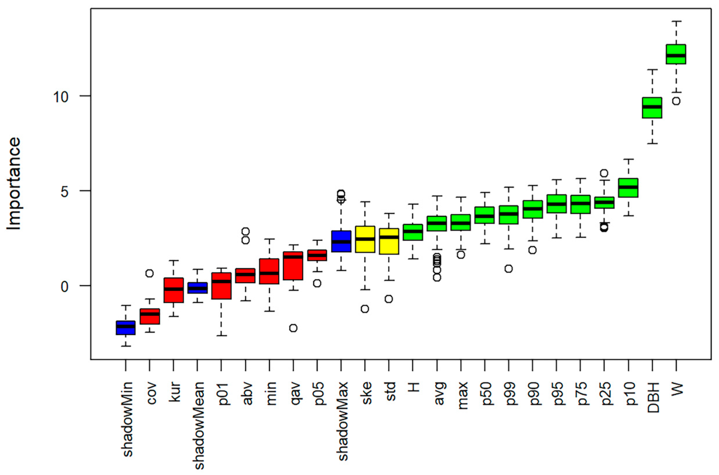
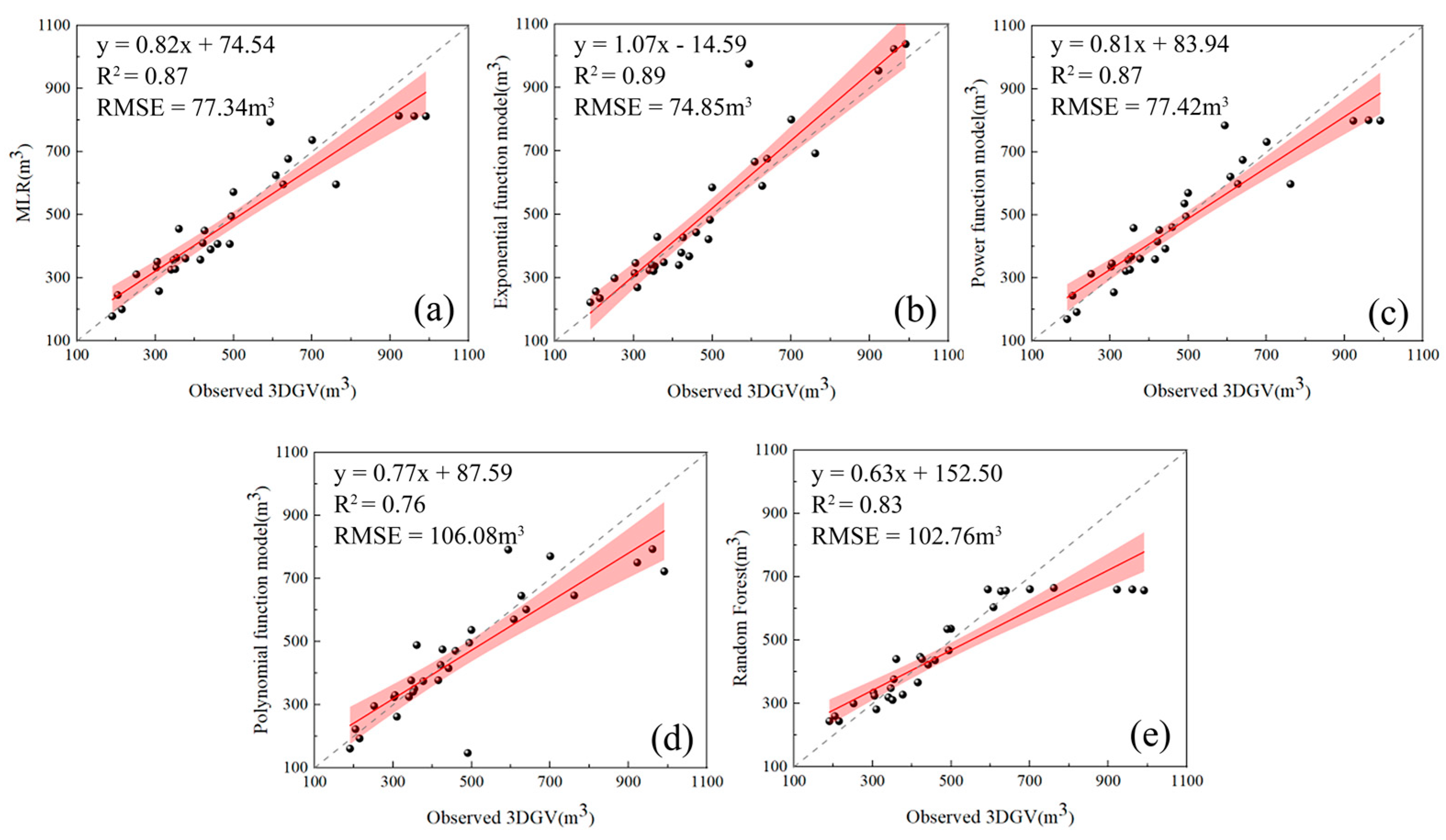
3.3. Variable Selection and Model Accuracy

The Boruta algorithm was used to screen the 21 variables. The Boruta algorithm established a reference line for shadow features and categorized variables into three types: important, tentative, and unimportant features. Figure 9 shows the importance distribution of each variable. Among them, the blue boxplot represents the shadow feature; green denotes the important feature selected by the algorithm. For example, the importance of W and DBH was much higher than the upper limit of shadow features, indicating that these variables had a significant impact on 3DGV. Yellow represents tentative features, indicating that the importance of ske and std overlapped with the distribution range of shadow features. These features require further verification through additional research. Red denotes unimportant features, such as qav and p05, whose importance fell below the maximum threshold of shadow features, indicating a weak correlation with 3DGV. Therefore, according to the screening results, the two most important variables, W and DBH, were selected for subsequent modeling.
Before modeling, the Shapiro–Wilk test was conducted to assess the normality of the 3DGV data. The result showed a p-value of 0.0512 (p > 0.05), indicating that the data follows a normal distribution, allowing for the application of a parametric model. In this study, five types of models were considered for 3DGV fitting. For the 30 sycamore samples, 70% were randomly selected as the training set and 30% as the validation set. The relationship between the 3DGV predicted by the five models and the observed 3DGV obtained using the CHCM is shown in Figure 10 and Table 3.
As shown in the results, all five models demonstrated strong predictive performance, with R2 values exceeding 0.75. Among them, the exponential function model performed the best performance, achieving the highest R2 and the lowest RMSE. This was followed by the MLR and the power function model, both showing an R2 of 0.87 and similar RMSE values. The random forest model showed slightly lower predictive accuracy. The polynomial function model with the lowest fitting accuracy had an R2 of 0.76 and an RMSE of 106.08 m3.

4. Discussion

4.1. Comparison of Different Methods

This study introduced the CHCM as a solution to the limitations of existing 3DGV estimation methods using TLS data. By dividing the canopy into upper and lower sections and applying convex hull and k-means clustering convex hulls, respectively, the CHCM effectively addressed the overestimation and underestimation issues observed in traditional methods. Comparison with five commonly used methods confirmed the CHCM’s adaptability to varying point cloud densities within the canopy, as well as its potential for accurate and non-destructive 3DGV estimation of urban trees.
As shown in Figure 8, the CHCM produced results closest to those of the frustum method. This is expected, as the frustum method was used as the reference in this study. However, there is a fundamental difference in the calculation methods between the frustum method and the CHCM, so the comparison remains valuable and ensures the comprehensiveness of the evaluation. The frustum method considers the tree canopy as a combination of numerous frustums and a cone. However, in practice, the shape of the canopy is irregular, which may lead to the inclusion of non-canopy space in the section volume calculation and reduce the overall stability of the results. In contrast, the CHCM does not require assumptions about the canopy shape, and its calculations better reflect the actual structure of the tree. The CHCM provides a more reliable and accurate method for estimating 3DGV, particularly in cases where the canopy shape varies significantly. The convex hull method produced the largest 3DGV among the six methods, and the result was significantly overestimated. This overestimation occurred because the convex hull method constructs a convex polyhedron around the entire tree canopy to calculate its 3DGV, thereby including all the gaps inside and around the tree canopy in the volume calculation [52].
The k-means clustering convex hulls method calculates the 3DGV by dividing the canopy into k clusters. However, it is important to note that the k-means algorithm is sensitive to initialization and outliers. To address this, we ran the algorithm multiple times with different random seeds and selected the result with the best compactness. Outliers were also removed during the individual tree segmentation and leaf–wood separation stages. These steps allowed us to retain the advantages of the k-means algorithm while reducing its limitations. Furthermore, the result of the k-means clustering convex hulls method was closely related to the number of clusters. Theoretically, a more accurate 3DGV can be obtained when the appropriate k1 is selected. However, due to the limited range of TLS data acquisition, the upper canopy information was occluded and could not be fully captured, resulting in missing point clouds, which led to a certain degree of underestimation. Compared with the k-means clustering convex hulls method, the proposed CHCM demonstrated superior performance in 3DGV estimation. The convex hull method was applied to replace the 3DGV calculation method in the upper part of the canopy. This adjustment compensates for the occlusion issue and results in more accurate 3DGV estimates.
The alpha-shape algorithm constructs a concave boundary that tightly wraps around the canopy points. This approach is advantageous when dealing with sparse or open canopies. However, in dense-canopy trees like sycamores, it may excessively remove internal spaces that are actually part of the crown, especially when the alpha value is not appropriately tuned [53,54]. This leads to an underestimation of 3DGV, as observed in our results. In addition, the accuracy of this method is highly sensitive to the choice of alpha parameter, which lacks a universal standard and often requires empirical tuning. In contrast, the CHCM reduced the influence of interstitial gaps within the canopy on the 3DGV, resulting in more accurate calculations.
The result of the voxel-based method was the smallest among all the methods. Like the alpha-shape algorithm, the voxel-based method often suffers from an underestimation of the 3DGV due to occlusion [55]. The voxel-based method calculates the 3DGV based on the internal structure of the tree canopy, which helps eliminate ineffective volumes within the canopy. It has certain advantages for the calculation of the 3DGV in the canopy of sparse branches and leaves with less internal structure occlusion. However, for sycamore with dense branches and leaves, the internal point cloud data of the tree canopy are missing due to occlusion, and the calculated result is often lower than the actual one. In addition, the accuracy of this method is highly sensitive to voxel size. There is no unified method to determine the voxel size in the current research. In contrast, the CHCM is more suitable for the 3DGV calculation of sycamore.
In general, the CHCM can effectively combine the characteristics of TLS point cloud data, thereby compensating for the overestimation or underestimation caused by other methods and providing more stable and accurate 3DGV estimates.

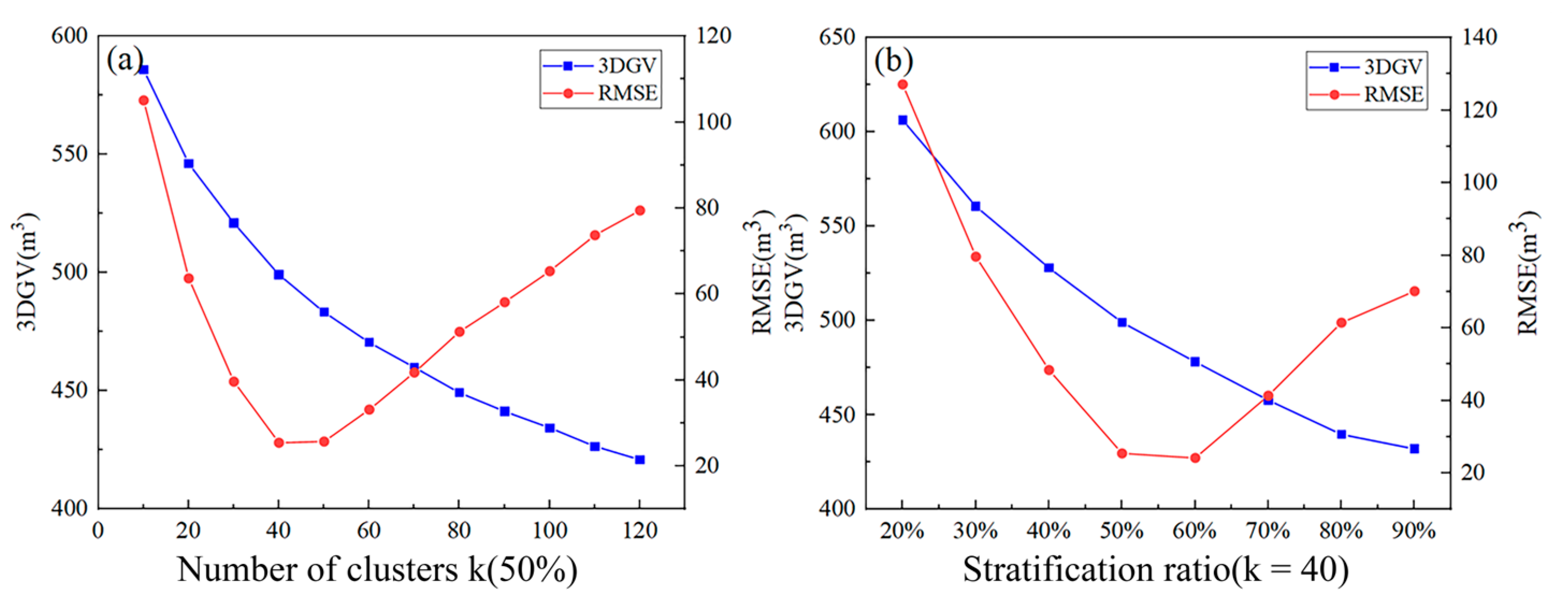
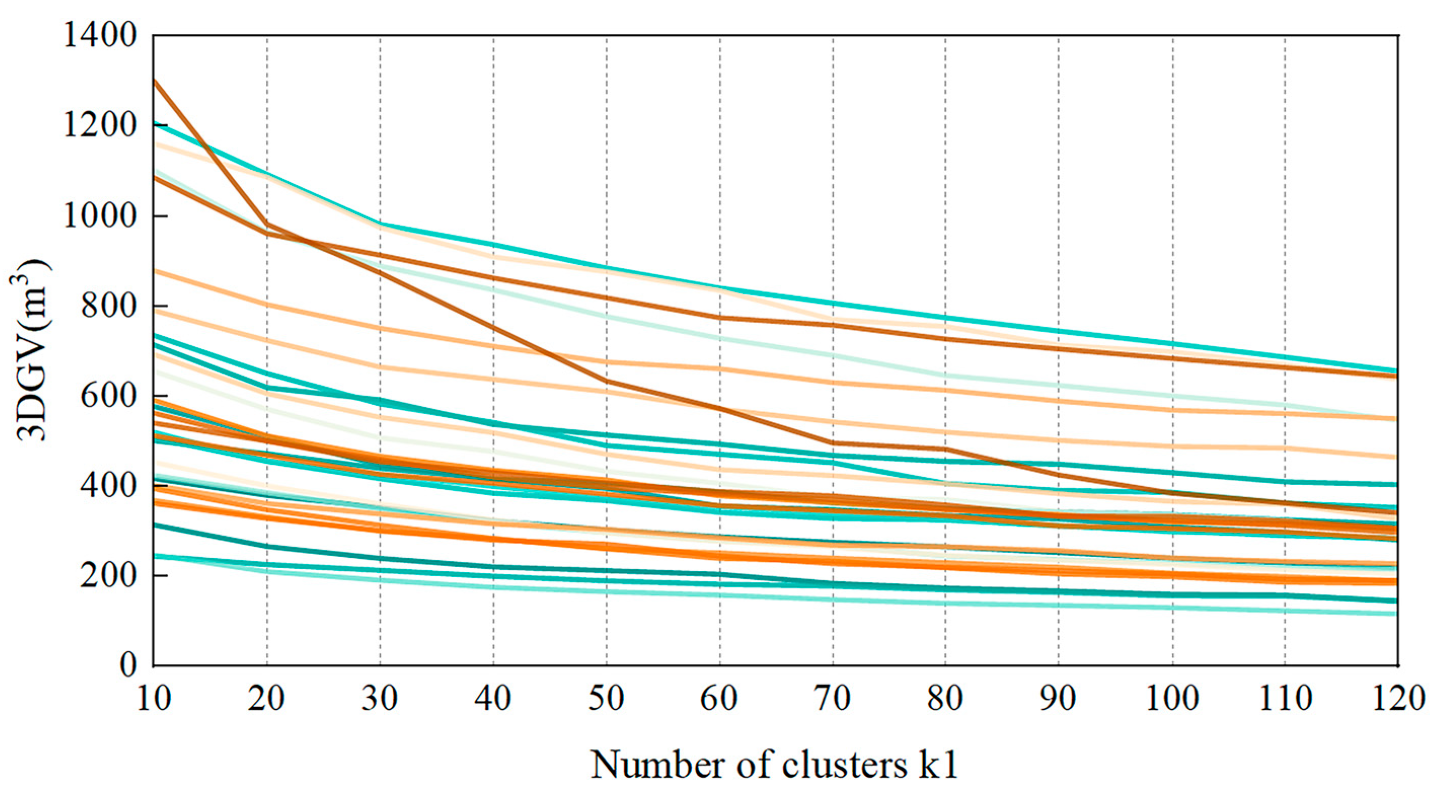
4.2. Parameter and Model Analysis

At present, 3DGV is not widely adopted in practical garden planning applications because it is difficult to obtain directly. The use of point cloud data has a high level of technical expertise and demands substantial programming skills, which hinders its efficient application by landscape professionals. Therefore, the significance of building a model in this study is to enable forestry workers who are not familiar with programming to calculate 3DGV quickly and conveniently.
Based on correlation and importance analysis, two optimal variables were ultimately selected. In previous studies, H, DBH, and W were frequently employed as variables for the construction of 3DGV models [56,57]. However, in this study, the optimal variables selected were W and DBH. The correlation between H and the 3DGV was relatively weak, and thus, H was excluded from the modeling process, which may be attributed to the artificial pruning of street trees. The sycamore is one of the most representative street trees in Nanjing. To meet the requirements of urban ecological management, the tree canopies were artificially pruned, altering the original shape. This intervention changed the original geometric characteristics of the trees. After pruning, the trees may take on the shape of a “broad crown and low height”, thus weakening the importance of H for 3DGV. Therefore, we speculated that for tree species with too much human interference, the conventional H, DBH, and W may no longer be universally applicable for 3DGV modeling and should instead be selected based on the specific structural characteristics of the target trees.
Five models were fitted in this study, all of which demonstrated reliable predictive performance. Among them, the exponential function model achieved the highest accuracy with an R2 of 0.89 and an RMSE of 74.85 m3. As shown in Figure 9, its fitting curve exhibited a slight upward curvature, in contrast to the straight line of the linear model. This nonlinearity may be due to the fact that canopy growth does not change linearly but gradually accelerates at different stages of the tree’s growth cycle. Artificial pruning may have further exacerbated this trend. These results suggest that for urban tree species whose canopy is greatly affected by human activities, the change of 3DGV tends to be nonlinear. The exponential function model can better capture the nonlinear relationship between the independent variables (W and DBH) and 3DGV, which can better explain the complexity of variables than the linear model. The MLR and the power function model had relatively lower fitting accuracy, with an R2 of 0.87. The random forest model (R2 = 0.83, RMSE = 102.76 m3) showed a relatively high RMSE. It could be that the model memorized the boundaries or extreme values while training on the data, leading to overfitting. Among the five models, the polynomial function model had the worst fitting accuracy. The polynomial function model is the most complex function in the parametric models, with relatively greater computational difficulty. Since the sample size in this study is relatively small, simpler models may be more appropriate.
Overall, the exponential function model demonstrated superior performance in explaining the variability of 3DGV and is suitable as an effective predictive model. The MLR and the power function model, as simple traditional statistical models, exhibited only slightly lower performance compared to the exponential function model and also have the advantage of being easily interpretable. Therefore, in practical applications, the exponential function model, MLR, and power function model can be regarded as preferred options for 3DGV estimation.

4.3. Research Deficiencies and Prospects

Based on the existing research, the calculation method of 3DGV was optimized through coupling, enhancing the accuracy of the calculation results and offering a novel idea for subsequent research. This study has several limitations. Firstly, due to the characteristics of TLS data, the point cloud density at the top of the canopy is relatively low, which may have affected the accuracy of the 3DGV estimates. In the future, more consideration could be given to other data acquisition devices, such as mobile laser scanning (MLS) and ALS, or multi-source data. Given the inability to ascertain the true value of 3DGV, we can only endeavor to obtain more accurate estimates. Thus, there remains significant potential for enhancing the calculation methodology of 3DGV. Future research could focus on optimizing algorithms or introducing new methods to enhance the accuracy and reliability of the estimation. The research object of this study is a single tree species, suggesting that the CHCM and subsequent fitting results may be specifically applicable to sycamores. The applicability of this method to other tree species requires further investigation.

5. Conclusions

Numerous studies have indicated that LiDAR point cloud data can be effectively utilized for estimating 3DGV. The advantage of LiDAR scanning lies in its ability to capture the three-dimensional structure of tree canopies without causing any damage to the trees, which is essential for accurate forestry assessments. For estimating the 3DGV of individual trees, TLS is frequently employed due to its ability to acquire detailed information from the lower portion of the canopy at close range, thereby facilitating precise segmentation of individual trees. Nevertheless, its limitations are also quite evident.
To enhance the precision of calculating the 3DGV of individual trees using TLS data, this study refined existing methodologies and introduced a novel approach—convex hull coupling k-means clustering convex hulls. To assess the reliability of this method, we calculated the 3DGV for 30 sycamore specimens and compared these results with those obtained from five established methods. The findings demonstrated that the CHCM was the most reliable among them. Based on the results generated by the CHCM, we selected five models to predict 3DGV at the individual tree level. While all models produced satisfactory fitting results, the exponential function model exhibited the highest accuracy (R2 = 0.89).
The accurate calculation and prediction of 3DGV are of vital significance for the study of tree biomass and the evaluation of the ecological environment. Street trees are an important part of urban ecological management, and sycamores are a representative street tree species in Nanjing. It is anticipated that the findings of this study can provide technical support for ecological management, environment assessment, and conservation efforts in Nanjing.

Author Contributions

Conceptualization, Y.Z.; methodology, Y.Z. and J.L.; software, J.L.; validation, Y.Z. and J.L.; formal analysis, Y.Z.; investigation, Y.Z. and J.L.; resources, Y.X.; data curation, Y.X.; writing—original draft preparation, Y.Z.; writing—review and editing, Y.Z. and J.L.; visualization, Y.Z.; supervision, Y.X.; project administration, Y.X.; funding acquisition, Y.X. All authors have read and agreed to the published version of the manuscript.

Funding

This research was funded by the Jiangsu Forestry Science and Technology Innovation and Extension Project (LYKJ [2021]14).

Data Availability Statement

Data will be made available on request.

Conflicts of Interest

The authors declare no conflicts of interest.

References

  1. Ćwik, A.; Wójcik, T.; Ziaja, M.; Wójcik, M.; Kluska, K.; Kasprzyk, I. Ecosystem Services and Disservices of Vegetation in Recreational Urban Blue-Green Spaces—Some Recommendations for Greenery Shaping. Forests 2021, 12, 1077. [Google Scholar] [CrossRef]
  2. Zhao, W. Research on Urban Green Space System Evaluation Index System. IOP Conf. Ser. Earth Environ. Sci. 2018, 208, 012061. [Google Scholar] [CrossRef]
  3. Hong, Z.; Xu, W.; Liu, Y.; Wang, L.; Ou, G.; Lu, N.; Dai, Q. Retrieval of Three-Dimensional Green Volume in Urban Green Space from Multi-Source Remote Sensing Data. Remote Sens. 2023, 15, 5364. [Google Scholar] [CrossRef]
  4. Bai, Y.; Liu, M.; Wang, W.; Xiong, X.; Li, S. Quantification of Urban Greenspace in Shenzhen Based on Remote Sensing Data. Remote Sens. 2023, 15, 4957. [Google Scholar] [CrossRef]
  5. Richards, D.; Wang, J.W. Fusing Street Level Photographs and Satellite Remote Sensing to Map Leaf Area Index. Ecol. Indic. 2020, 115, 106342. [Google Scholar] [CrossRef]
  6. Huang, J.; Song, P.; Liu, X.; Li, A.; Wang, X.; Liu, B.; Feng, Y. Carbon Sequestration and Landscape Influences in Urban Greenspace Coverage Variability: A High-Resolution Remote Sensing Study in Luohe, China. Forests 2024, 15, 1849. [Google Scholar] [CrossRef]
  7. Zhou, J.; Sun, T. Study on Remote Sensing Model of Three-Dimensional Green Biomass and the Estimation of Environmental Benefits of Greenery. Remote Sens. Environ. China 1995, 3, 162–174. [Google Scholar] [CrossRef]
  8. Li, F.; Li, M.; Feng, X. High-Precision Method for Estimating the Three-Dimensional Green Quantity of an Urban Forest. J. Indian Soc. Remote Sens. 2021, 49, 1407–1417. [Google Scholar] [CrossRef]
  9. Giannico, V.; Stafoggia, M.; Spano, G.; Elia, M.; Dadvand, P.; Sanesi, G. Characterizing green and gray space exposure for epidemiological studies: Moving from 2D to 3D indicators. Urban For. Urban Green. 2022, 72, 127567. [Google Scholar] [CrossRef]
  10. Kong, L.; Wang, X.; Zhou, X. Living Vegetation Volume Estimation of Urban Street Trees by Integrating Street View and Remote Sensing Images. J. Fuzhou Univ. (Nat. Sci. Ed.) 2025, 53, 1–8. [Google Scholar] [CrossRef]
  11. Miguel, E.; Rezende, A.; Pereira, R.; Azevedo, G.; Mota, F.; Souza, A.; Joaquim, M. Modeling and Prediction of Volume and Aereal Biomass of the Tree Vegetation in a Cerradao Area of Central Brazil. Interciencia 2017, 42, 21–27. [Google Scholar]
  12. Verma, N.K.; Lamb, D.W.; Reid, N.; Wilson, B. Comparison of Canopy Volume Measurements of Scattered Eucalypt Farm Trees Derived from High Spatial Resolution Imagery and LiDAR. Remote Sens. 2016, 8, 388. [Google Scholar] [CrossRef]
  13. Miranda-Fuentes, A.; Llorens, J.; Gamarra-Diezma, J.L.; Gil-Ribes, J.A.; Gil, E. Towards an Optimized Method of Olive Tree Crown Volume Measurement. Sensors 2015, 15, 3671–3687. [Google Scholar] [CrossRef] [PubMed]
  14. Xu, D.; Wang, H.; Xu, W.; Luan, Z.; Xu, X. LiDAR Applications to Estimate Forest Biomass at Individual Tree Scale: Opportunities, Challenges and Future Perspectives. Forests 2021, 12, 550. [Google Scholar] [CrossRef]
  15. Luo, T.; Rao, S.; Ma, W.; Song, Q.; Cao, Z.; Zhang, H.; Xie, J.; Wen, X.; Gao, W.; Chen, Q.; et al. YOLOTree-Individual Tree Spatial Positioning and Crown Volume Calculation Using UAV-RGB Imagery and LiDAR Data. Forests 2024, 15, 1375. [Google Scholar] [CrossRef]
  16. Calders, K.; Adams, J.; Armston, J.; Bartholomeus, H.; Bauwens, S.; Bentley, L.P.; Chave, J.; Danson, M.; Demol, M.; Disney, M.; et al. Terrestrial Laser Scanning in Forest Ecology: Expanding the Horizon. Remote Sens. Environ. 2020, 251, 112102. [Google Scholar] [CrossRef]
  17. Yang, Y.; Shen, X.; Cao, L. Estimation of the Living Vegetation Volume (LVV) for Individual Urban Street Trees Based on Vehicle-Mounted LiDAR Data. Remote Sens. 2024, 16, 1662. [Google Scholar] [CrossRef]
  18. Hong, Z.; Xu, W.; Liu, Y.; Wang, L.; Ou, G.; Lu, N.; Dai, Q. Estimation of the Three-Dimension Green Volume Based on UAV RGB Images: A Case Study in YueYaTan Park in Kunming, China. Forests 2023, 14, 752. [Google Scholar] [CrossRef]
  19. Olsoy, P.J.; Glenn, N.F.; Clark, P.E.; Derryberry, D.R. Aboveground Total and Green Biomass of Dryland Shrub Derived from Terrestrial Laser Scanning. ISPRS J. Photogramm. Remote Sens. 2014, 88, 166–173. [Google Scholar] [CrossRef]
  20. Colaço, A.F.; Trevisan, R.G.; Molin, J.P.; Rosell-Polo, J.R.; Escolà, A. Orange Tree Canopy Volume Estimation by Manual and LiDAR-Based Methods. Adv. Anim. Biosci. 2017, 8, 477–480. [Google Scholar] [CrossRef]
  21. Li, X.; Tang, L.; Peng, W.; Chen, J.; Ma, X. Estimation Method of Urban Green Space Living Vegetation Volume Based on Backpack Light Detection and Ranging. Chin. J. Appl. Ecol. 2022, 33, 2777–2784. [Google Scholar] [CrossRef]
  22. Korhonen, L.; Vauhkonen, J.; Virolainen, A.; Hovi, A.; Korpela, I. Estimation of Tree Crown Volume from Airborne Lidar Data Using Computational Geometry. Int. J. Remote Sens. 2013, 34, 7236–7248. [Google Scholar] [CrossRef]
  23. Wang, J.Y. Calculation Method of Single Tree Canopy Volume Based on LiDAR Technology. Master’s Thesis, Henan Polytechnic University, Jiaozuo, China, 2022. [Google Scholar]
  24. Fernández-Sarría, A.; Martínez, L.; Velázquez-Martí, B.; Sajdak, M.; Estornell, J.; Recio, J.A. Different Methodologies for Calculating Crown Volumes of Platanus hispanica Trees Using Terrestrial Laser Scanner and a Comparison with Classical Dendrometric Measurements. Comput. Electron. Agric. 2013, 90, 176–185. [Google Scholar] [CrossRef]
  25. Huang, F.; Peng, S.; Chen, S.; Cao, H.; Ma, N. VO-LVV–A Novel Urban Regional Living Vegetation Volume Quantitative Estimation Model Based on the Voxel Measurement Method and an Octree Data Structure. Remote Sens. 2022, 14, 855. [Google Scholar] [CrossRef]
  26. Wang, K.; Kumar, P. Characterizing Relative Degrees of Clumping Structure in Vegetation Canopy Using Waveform LiDAR. Remote Sens. Environ. 2019, 232, 111281. [Google Scholar] [CrossRef]
  27. Zhu, H.; Nan, X.; Kang, N.; Li, S. How Much Visual Greenery Can Street Trees Generate from a Humanistic Perspective? An Attempt to Quantify the Canopy Green View Index Based on Tree Morphology. Forests 2024, 15, 88. [Google Scholar] [CrossRef]
  28. Liu, J.; Zheng, B. A Simulation Study on the Influence of Street Tree Configuration on Fine Particulate Matter (PM2.5) Concentration in Street Canyons. Forests 2023, 14, 1550. [Google Scholar] [CrossRef]
  29. Sun, X.; Qiu, Y.; Qi, H.; Lu, W.; Tian, J.; Chen, S.; Xu, Y. Improving the Ecological Benefits Evaluation on Urban Street Trees: Development of a Living Vegetation Volume Quantifying Framework with Multi-Source Data. Ecol. Indic. 2024, 158, 111367. [Google Scholar] [CrossRef]
  30. Gratani, L.; Vasheka, O.; Bigaran, F. Phenotypic Plasticity of Platanus acerifolia (Platanaceae): Morphological and Anatomical Trait Variations in Response to Different Pollution Levels in Rome. Mod. Phytomorphology 2020, 14, 55–63. [Google Scholar] [CrossRef]
  31. Hang, X.; Li, Y.; Luo, X.; Xu, M.; Han, X. Assessing the Ecological Quality of Nanjing during Its Urbanization Process by Using Satellite, Meteorological, and Socioeconomic Data. J. Meteorol. Res. 2020, 34, 280–293. [Google Scholar] [CrossRef]
  32. Massetti, L. Assessing the Impact of Street Lighting on Platanus × acerifolia Phenology. Urban For. Urban Green. 2018, 34, 71–77. [Google Scholar] [CrossRef]
  33. Liu, M.Z. Research on Organic Renewal Design Strategy of Street Tree Landscape in Nanjing Abstract. Master’s Thesis, Nanjing Forestry University, Nanjing, China, 2023. [Google Scholar]
  34. Vicari, M.B.; Disney, M.; Wilkes, P.; Burt, A.; Calders, K.; Woodgate, W. Leaf and Wood Classification Framework for Terrestrial LiDAR Point Clouds. Methods Ecol. Evol. 2019, 10, 680–694. [Google Scholar] [CrossRef]
  35. Wang, D.; Momo Takoudjou, S.; Casella, E. LeWoS: A Universal Leaf-wood Classification Method to Facilitate the 3D Modelling of Large Tropical Trees Using Terrestrial LiDAR. Methods Ecol. Evol. 2020, 11, 376–389. [Google Scholar] [CrossRef]
  36. Ali, M.; Lohani, B.; Hollaus, M.; Pfeifer, N. Benchmarking Geometry-Based Leaf-Filtering Algorithms for Tree Volume Estimation Using Terrestrial LiDAR Scanners. Remote Sens. 2024, 16, 1021. [Google Scholar] [CrossRef]
  37. Xu, W.; Feng, Z.; Su, Z.; Xu, H.; Jiao, Y.; Deng, O. An Automatic Extraction Algorithm for Individual Tree Crown Projection Area and Volume Based on 3D Point Cloud Data. Spectrosc. Spectr. Anal. 2014, 34, 465–471. [Google Scholar] [CrossRef]
  38. Ghanbari Parmehr, E.; Amati, M. Individual Tree Canopy Parameters Estimation Using UAV-Based Photogrammetric and LiDAR Point Clouds in an Urban Park. Remote Sens. 2021, 13, 2062. [Google Scholar] [CrossRef]
  39. Rodríguez-Lozano, B.; Rodríguez-Caballero, E.; Maggioli, L.; Cantón, Y. Non-Destructive Biomass Estimation in Mediterranean Alpha Steppes: Improving Traditional Methods for Measuring Dry and Green Fractions by Combining Proximal Remote Sensing Tools. Remote Sens. 2021, 13, 2970. [Google Scholar] [CrossRef]
  40. Li, X.; Tang, L.; Huang, H.; Chen, C.; He, J. A Method for Estimating Living Vegetation Volume of Urban Trees based on Point Cloud Data. Remote Sens. Technol. Appl. 2022, 37, 1119–1127. [Google Scholar]
  41. Zhou, L.; Li, X.; Zhang, B.; Xuan, J.; Gong, Y.; Tan, C.; Huang, H.; Du, H. Estimating 3D Green Volume and Aboveground Biomass of Urban Forest Trees by UAV-Lidar. Remote Sens. 2022, 14, 5211. [Google Scholar] [CrossRef]
  42. Zhu, Z.; Kleinn, C.; Nölke, N. Towards Tree Green Crown Volume: A Methodological Approach Using Terrestrial Laser Scanning. Remote Sens. 2020, 12, 1841. [Google Scholar] [CrossRef]
  43. Lin, W.; Meng, Y.; Qiu, Z.; Zhang, S.; Wu, J. Measurement and Calculation of Crown Projection Area and Crown Volume of Individual Trees Based on 3D Laser-Scanned Point-Cloud Data. Int. J. Remote Sens. 2017, 38, 1083–1100. [Google Scholar] [CrossRef]
  44. Gupta, S.; Weinacker, H.; Koch, B. Comparative Analysis of Clustering-Based Approaches for 3-D Single Tree Detection Using Airborne Fullwave Lidar Data. Remote Sens. 2010, 2, 968–989. [Google Scholar] [CrossRef]
  45. Li, L.; Li, D.; Zhu, H.; Li, Y. A Dual Growing Method for the Automatic Extraction of Individual Trees from Mobile Laser Scanning Data. ISPRS J. Photogramm. Remote Sens. 2016, 120, 37–52. [Google Scholar] [CrossRef]
  46. Wu, B.; Yu, B.; Yue, W.; Shu, S.; Tan, W.; Hu, C.; Huang, Y.; Wu, J.; Liu, H. A Voxel-Based Method for Automated Identification and Morphological Parameters Estimation of Individual Street Trees from Mobile Laser Scanning Data. Remote Sens. 2013, 5, 584–611. [Google Scholar] [CrossRef]
  47. Huang, M.; Wei, P.; Liu, X. An Efficient Encoding Voxel-Based Segmentation (EVBS) Algorithm Based on Fast Adjacent Voxel Search for Point Cloud Plane Segmentation. Remote Sens. 2019, 11, 2727. [Google Scholar] [CrossRef]
  48. Kursa, M.B.; Rudnicki, W.R. Feature selection with the Boruta package. J. Stat. Softw. 2010, 36, 1–13. [Google Scholar] [CrossRef]
  49. Ahmadpour, H.; Bazrafshan, O.; Rafiei-Sardooi, E.; Zamani, H.; Panagopoulos, T. Gully Erosion Susceptibility Assessment in the Kondoran Watershed Using Machine Learning Algorithms and the Boruta Feature Selection. Sustainability 2021, 13, 10110. [Google Scholar] [CrossRef]
  50. Degenhardt, F.; Seifert, S.; Szymczak, S. Evaluation of variable selection methods for random forests and omics data sets. Brief. Bioinform. 2019, 20, 492–503. [Google Scholar] [CrossRef]
  51. Cheng, G.; Wang, J.; Yang, J.; Zhao, Z.; Wang, L. Calculation Method of 3D Point Cloud Canopy Volume Based on Improved α-shape Algorithm. Trans. Chin. Soc. Agric. Mach. 2021, 52, 175–183. [Google Scholar] [CrossRef]
  52. Fernández-Sarría, A.; Velázquez-Martí, B.; Sajdak, M.; Martínez, L.; Estornell, J. Residual Biomass Calculation from Individual Tree Architecture Using Terrestrial Laser Scanner and Ground-Level Measurements. Comput. Electron. Agric. 2013, 93, 90–97. [Google Scholar] [CrossRef]
  53. Vauhkonen, J.; Seppänen, A.; Packalén, P.; Tokola, T. Improving Species-Specific Plot Volume Estimates Based on Airborne Laser Scanning and Image Data Using Alpha Shape Metrics and Balanced Field Data. Remote Sens. Environ. 2012, 124, 534–541. [Google Scholar] [CrossRef]
  54. Zhen, Z.; Quackenbush, L.J.; Zhang, L. Trends in Automatic Individual Tree Crown Detection and Delineation—Evolution of LiDAR Data. Remote Sens. 2016, 8, 333. [Google Scholar] [CrossRef]
  55. Lecigne, B.; Delagrange, S.; Messier, C. Exploring Trees in Three Dimensions: VoxR, a Novel Voxel-Based R Package Dedicated to Analysing the Complex Arrangement of Tree Crowns. Ann. Bot. 2018, 121, 589–601. [Google Scholar] [CrossRef] [PubMed]
  56. Sun, X.; Xu, S.; Hua, W.; Tian, J.; Xu, Y. Feasibility Study on the Estimation of the Living Vegetation Volume of Individual Street Trees Using Terrestrial Laser Scanning. Urban For. Urban Green. 2022, 71, 127553. [Google Scholar] [CrossRef]
  57. Wang, P.P. The Estimation of Living Vegetation Volume in the Ring Park around Hefei City Based on TLS and Landsat8. Master’s Thesis, Anhui Agricultural University, Hefei, China, 2018. [Google Scholar]
Figure 1. Overview of the study area: (a) location of Nanjing; (b) location of the study area; (c) TLS point cloud of the study area; and (d) a map image of the study area.
Forests 16 00690 g001
Figure 2. Distribution of TLS stations.
Forests 16 00690 g002
Figure 3. A 3DGV calculation: (a) point cloud of the sycamore canopy; (b) the convex hull method fitting of the 3DGV; (c) the k-means clustering convex hulls method fitting of the 3DGV; and (d) the CHCM method fitting of the 3DGV.
Forests 16 00690 g003
Figure 4. Technical flowchart of this study.
Forests 16 00690 g004
Figure 5. Optimization of parameters: (a) determination of the optimal k (stratification ratio = 50%) and (b) determination of the optimal stratification ratio (k = 40).
Forests 16 00690 g005
Figure 6. Results of 3DGV in the CHCM.
Forests 16 00690 g006
Figure 7. The 3DGV calculated by k-means clustering convex hulls method with different k1.
Forests 16 00690 g007
Figure 8. The 3DGV distribution of 30 trees by six methods (definitions: M1, the CHCM; M2, the frustum method; M3, the convex hull method; M4, the k-means clustering convex hulls; M5, the alpha-shape algorithm; M6, the voxel-based method).
Forests 16 00690 g008
Figure 9. The variable selection results of Boruta algorithm.
Forests 16 00690 g009
Figure 10. Accuracy verification of the different models fitting: (a) MLR; (b) exponential function model; (c) power function model; (d) polynomial function model; and (e) random forest.
Forests 16 00690 g010
Table 1. Parameter settings of RIEGL VZ-400i.
Scanning ParameterSpecification
Laser pulse repetition rate1200 kHz
Accuracy/Repeatability5 mm/3 mm
Maximum measurement range800 m
Minimum measurement range1.5 m
Horizontal field of view360°
Horizontal scan speed0–150°/s
Vertical field of view100° (+60°/−40°)
Vertical scan speed3~240 lines/s
Table 2. Description of the LiDAR variables.
LiDAR VariablesDescriptionStatistical Methods
Height-basedp01, p05, p10, p25, p50, p75, p90, p95, p99The percentiles (p01, p05, p10, p25, p50, p75, p90, p95, p99) of the canopy height distribution of the first returns.Extracted by LAStools
minMinimum height above ground of all first returns.
maxMaximum height above ground of all first returns.
avgMean height above ground of all first returns.
stdThe standard deviation of the heights of all points.
skeThe skewness of the heights of all points.
kurThe kurtosis of the heights of all points.
qavThe average square height of all points.
abvThe number of points that actually are above the cutoff and are participating in the computation.
Density-basedCanopy cover(cov)Percentages of first returns above the cover at breast height.Extracted by LAStools
Canopy-basedHTree height.Extracted from the point clouds
WTree crown width: the average of the width in the north–south and east–west directions.
DBHDiameter at breast height.Field surveys
Table 3. Different models for estimating 3DGV accuracy.
ModelRMSE/m3
MLR0.8777.34
Exponential function model0.8974.85
Power function model0.8777.42
Polynomial function model0.76106.08
Random forest0.83102.76
Disclaimer/Publisher’s Note: The statements, opinions and data contained in all publications are solely those of the individual author(s) and contributor(s) and not of MDPI and/or the editor(s). MDPI and/or the editor(s) disclaim responsibility for any injury to people or property resulting from any ideas, methods, instructions or products referred to in the content.

