Abstract
Dioecious plants have different needs for natural resources due to sex differences, which can lead to skewed sex ratios. Clonal growth facilitates and optimizes resources of clonal plants. So, dioecious plants show inter-sex differences in clonality. However, it is unclear how the clonality varies between female and male plants when they exhibit skewed sex ratios along an altitudinal gradient. Here, we investigated the sex ratio and clonality of Hippophae tibetana populations growing at three altitudes in the alpine meadow. We founded that (i) H. tibetana growing at different altitudes mainly consisted of II and III age classes, with a significantly male-biased sex ratio observed at a low altitude, a female-biased ratio at a middle altitude, and no significant sex-bias in the population at a high altitude. (ii) The population distribution was generally random at both low and high altitudes, while clustered at middle altitudes with an increasing scale. Meanwhile, the male and female populations at a low altitude showed a negative correlation, while the male and female at a middle altitude only showed a negative correlation at a 0–0.5 m scale, and spatial independence with increasing scales. (iii) Females of H. tibetana had a strong clonal capacity than male plants at a middle altitude, while the opposite was observed at a low altitude. The number of males of H. tibetana growing at a low altitude and with higher clonal diversity were higher than females at mid altitude. Our findings will contribute to the understanding of the sexual dimorphism exhibited by dioecious plants as well as the importance of a clonal adaptation in response to environmental change.
1. Introduction
For clonal plants, the clonal diversity and clonal structure can significantly increase plant fitness and buffer against environmental heterogeneity [1]. Thus, how many clones are included in a plant population (clonal diversity) and how different clones are spatially distributed (clonal structure) can greatly influence populations [2]. Clonal plants can adjust their resource acquisition methods through plasticity changes, which can affect the clonal structure and clonal diversity of the clonal plant, thus the study of plasticity changes is of ecological importance. These have long been important topics in plant ecology and evolution [3]. A key tool in these studies is the use of molecular markers to allow, without regard to the phenotype, an unbiased comparison of the adaptation of organisms to their environment, its genetic basis and its effect on evolution [4]. This is the most reliable way for characterizing the genetic structure of clonal populations [5,6]. Therefore, by utilizing advanced molecular marker techniques, we were able to accurately characterize the clonal structure and diversity of male and female populations of Hippophae tibetana Schltdl at different altitudes. This provided novel insights into the sex-specific ecological adaptation of H. tibetana populations and new evidence for the study of sex-specific ecological adaptation in clonal plants.
The sex ratio and spatial distribution pattern can reflect the adaptation of dioecious plant populations to the environment to a certain extent [7]. Classic sex ratio theory suggests that natural selection will balance the sex ratio of the population when the reproductive costs of female and male offspring are equal [8]. However, dioecious plants exhibit sexual dimorphism in terms of primary sexual traits and vegetative traits (secondary sexual dimorphism) in order to better adapt to their environments [9], which can lead to dioecious plants having significantly biased sex ratios [10,11,12,13]. So, changes in sex ratios of dioecious plants can provide a better understanding of their adaptations to the environment, and the spatial distribution pattern of populations can also reflect the survival strategies and adaptive mechanisms adopted by populations to adapt to the environment [14], which is important for the study of intraspecific interactions and plant–environment relationships [15]. Therefore, studying the sex ratio structure and sex-related spatial patterns in dioecious plants contributes to a deeper understanding of population dynamics. Simultaneously, we systematically studied the relationship between clonality and the sex ratio in H. tibetana populations at different altitude gradients. It was beneficial for revealing how environmental changes along the altitudinal gradient shaped the clonal growth strategies of male and female plants, thereby influencing the sex ratio. This comprehensive analysis provided a unique perspective on the adaptation mechanisms of dioecious plants in complex alpine meadow ecosystems, which had not been thoroughly explored in previous studies.
Elaeagnaceae includes multiple genera, among which Hippophae is rather remarkable. The common species of this genus include Hippophae rhamnoides ssp. sinensis, Hippophae rhamnoides ssp. mongolica, etc. As a member of the Hippophae genus, H. tibetana is a dioecious shrub and it is a typical alpine plant that occupies a unique position in the ecosystem [16]. It can sexually reproduce assisted by wind [17] and can also spread via ramets. This woody plant grows at a high altitude across the Qinghai–Tibetan Plateau and Himalayan region [18] and is often distributed as large thickets. It is tolerant of extreme environmental conditions, demonstrating a remarkable adaptability to cold, drought, low supplies of nitrogen, and exposure to intense UV-B ultraviolet light stress (280–315 nm;) [19]. It is a pioneer plant that can survive in extreme habitats and has important ecological and economic values [20]. It is used for soil and water conservation and phytoremediation in mine wastelands and is also an important resource plant. It has been widely planted in the northwest of China for desert greening and as an ingredient in food [21], etc. H. tibetana provides an ideal study system to investigate the sex-specific differences of sex ratios and clonality in populations of the QTP along different altitudes. To date, although some studies have been conducted to investigate the variation of the sex ratio and clonality along altitudes in different species [22,23], the number of species involved and the content of the studies are relatively small [24], and in order to be clearer on this issue, more experimental evidence is needed, including changes in the clonal structure, diversity, and sex ratios of natural populations along different altitudes, or their relationship with them and sex-specific differences.
In this study, we examined the cloning abilities of the dioecious H. tibetana population at three different altitudes on the eastern edge of the QTP. We used molecular markers to characterize the genetic structure of clonal populations to reveal their sex ratio pattern and clonal structure along the altitudinal gradient and addressed the following questions: (i) Is there any variation in sex ratios along the altitudinal gradient? (ii) What is the spatial distribution of H. tibetana? (iii) How does the clonal structure and clonal diversity of female and male populations of H. tibetana vary along the altitudinal gradient?
2. Materials and Methods
2.1. Study Area
The study area is located in Tianzhu Tibetan Autonomous County, Wuwei City, Gansu Province, in the Qilian Mountains on the northeastern edge of the QTP. The field sites have a geographical span of 103.7°–104.7° E, 36.6°–37.6° N, and range in altitude between 2040 and 4873 m. This region experiences a continental plateau monsoon climate, with an annual average temperature of −0.2–1.3 °C, an accumulated temperature of ≥0 °C of 1327.7–1738.2 °C, and an annual precipitation of 265.5–630 mm [25]. There are only warm and cold seasons, with the latter extending over 7 months. The climate data described herein are sourced from regional meteorological stations and pertain to the broader area within which our study plots are located. The soil is mainly mountainous chernozem, chestnut soil, subalpine meadow soil, and alpine meadow soil. In this area, H. tibetana is the dominant plant species in the community (Figure 1), and other plant species include Potentilla fruticosa, Salix sinica, Polygonum viviparum, Leymus secalinus, Carex korshinskyi, Oxytropis ochrocepha, and Elymus sibiricus.
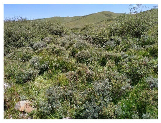
Figure 1.
H. tibetana community in Qilian Mountains of Qinghai–Tibetan Plateau.
2.2. Sample Plot Setting and Investigation
In August 2020, based on multiple field investigations, in Zhuaxixiulong Town, Tianzhu County, three field sites with a relatively concentrated distribution of H. tibetana were selected, and three fixed field sites were set up according to low altitude, middle altitude, and high altitude, namely the Zhuaxixiulong Scenic Area (102°48′10.90″ E, 37°9′32.02″ N, 2868 m), Honggeda Village (102°40′29.69″ E, 37°14′5.43″ N, 3012 m), and Baishuikou Village (102°32′1.77″ E, 37°15′16.54″ N, 3244 m). Four 5 m×5 m plots were selected at each site. We picked the young leaves of H. tibetana, marked the serial numbers and genders, and dried them on silica gel. Meanwhile, due to workload limitations and the absence of sex ratio bias at high altitudes, we only selected one plot of 5 m × 5 m in both the low-altitude and medium-altitude areas, respectively, and divided them into small sample grids of 1 m × 1 m by using the adjacent grid method. This was used to measure and record the two-dimensional space of each H. tibetana plant relative to the origin of the coordinates. We identified the gender of H. tibetana by flowers and fruits, and if there were no flowers and fruits on a plant, we identified it by the mature ramets attached to the root through digging.
2.3. Population Counting and Sex Ratio Calculation
The number of male and female individuals at different altitudes was counted and the significance of the sex ratio (female/male) deviating from the null hypothesis of 1:1 was tested. H. tibetana plants were individual ramets and the sex ratio was calculated with ramet numbers [26].
In order to understand the specific sex ratio pattern in H. tibetana populations at different altitudes, the number of male and female plants at different age levels was counted and the significance of the sex ratio (female/male) deviating from the null hypothesis of 1:1 was tested.
Since plant size and age are closely related, and the growth and age of the same species in the same habitat have a consistent response to the environment [27], the use of plant size instead of age was a common method to study the age structure of populations. However, due to the dwarfing of H. tibetana plants, the relationship between their basal diameter and age is even closer. So, we adopted the method of using basal diameter instead of age to study the age structure of the H. tibetana population. In this study, the minimum basal diameter (BD) of H. tibetana female plants was about 0.3 cm. Combined with the actual field investigation, the basal diameter (BD) was divided into 0.3 cm as a level, which can be divided into: (BD ≤ 0.3 cm), II (0.3 cm < BD ≤ 0.6 cm), III (0.6 cm < BD ≤ 0.9 cm), IV (0.9 cm < BD ≤ 1.2 cm), V (1.2 cm < BD ≤ 1.5 cm), VI (1.5 cm < BD ≤ 1.8 cm), and VII (BD > 1.8 cm), totaling seven age classes.
2.4. Population Spatial Distribution Types and Spatial Correlation
Based on the obtained coordinate position of each individual in the obtained spatial distribution point map, the Ripley’s K function in the point pattern analysis method was used to analyze the spatial distribution types of H. tibetana populations at different altitudes and the spatial correlation of female and male populations [28].
The expression of the univariate K(r) function is as follows:
where r is the spatial scale, A the quadrant area, n the number of plant individuals in the quadrant, I the exponential function, Uij the distance between points i and j, and Wij is the area with i as the radius and Uij as the center, with the ratio of the circumference of a circle to the area A [29]. After Besag corrected the K(r) function, the L(r) function was obtained:
The expression of the two-variable K12(r) function is as follows:
where n1 and n2, respectively, represent the number of female and male individuals in area A [30]. The other parameters in the formula are the same as for K(r). Afterwards, K12(r) was used to calculate L12(r) [31], as follows:
Based on the two-dimensional coordinate point information of the plants in the population, data analysis was completed with Programita 2018 software: the spatial scale was set to half of the minimum side length of the sample plot (250 cm), the step length was set to 1 m, and 99 simulations were repeated to obtain the 99% confidence intervals. From the Monte Carlo simulated confidence intervals, we obtained two top and bottom envelopes. For the distribution pattern of populations at different altitudes, when L(r) was above the top envelope, aggregated distribution was identified; when L(r) was between the two envelopes, random distribution was identified; and when L(r) was below the bottom envelope, uniform distribution was assumed. For the space between male and female interspecific spatial correlation, when L12(r) > upper envelops, the correlation between the two subjects is positive; when lower envelopes < L12(r) < upper envelopes, the correlation indicates that the two subjects are not related; and when L12(r) < lower envelops, the correlation between the two subjects is negative [32].
2.5. DNA Extraction and Detection
The improved CTAB method [33] was used to extract total genomic DNA from the young leaves of H. tibetana. The DNA was diluted with ddH2O to approximately 50 ng μL−1. A NanoDrop ultra-micro spectrophotometer was used to evaluate the purity and concentration of the extracted DNA which was then stored at 4 °C for later use.
2.6. PCR Amplification and SSR Primer Screening
H. tibetana did not show sex ratio bias at high altitude, so we did not study it further. We used 26 pairs of H. tibetana primers [34,35,36], and selected 20 individuals from low and middle altitudes for screening clonal diversity. Polymerase chain reaction was performed in a 25 μL reaction system: 2 μL of DNA template, 1 μL of upstream and downstream primers, and 2× TaqPCRMix 12.5 μL and 8.5 μL of ddH2O. The reaction was carried out on a PCR machine (Suzhou Dongsheng Xingye Scientific Instruments Co., Ltd., Suzhou, China). The SSR-PCR amplification program carried out pre-denaturation at 98 °C for 30 s, followed by 36 cycles of denaturation at 98 °C for 10 s, annealing for 45 s, and extension at 72 °C for 1 min; after the cycle, extension at 72 °C for 2 min, and then storing at 4 °C.
Polyacrylamide gel electrophoresis with a DYY-2 double-plate vertical electrophoresis tank (Beijing Liuyi Factory, Beijing, China) was used to detect the PCR product. Loading buffer (5 μL) was added at a ratio of 1:6 to 25 μL of the PCR product before spotting out. The sample volume was 5 μL, and electrophoresis was carried out in a denaturing polyacrylamide gel with a volume fraction of 6%, using 1× TBE buffer (Beijing Solarbio Science & Technology Co., Ltd., Beijing, China) as the electrolyte, a constant voltage of 350–400 V, and electrophoresis for 2–2.5 h.
2.7. Data Analysis
SPSS22.0 software was used to analyze sex ratios, and a chi-square test was used to test the significance of sex ratio (female/male) deviation from the null hypothesis of 1:1. According to the electrophoresis data, SSR is a co-dominant molecular marker, so the band records are expressed in homozygous or heterozygous manner. For example, if the allele length of a locus is 110 bp and 112 bp, then the homozygous band is recorded as 110 110, and the hybrid band is 110 112. Using CERVUS3.0 [37] software, the read band data were analyzed to determine the polymorphism of the SSR site. The SSR data processing macro program Data Formater was used to convert the original bp data into the 0 and 1 matrices required by Popgen 32 software and NTsys 2.10e software.
Popgen32 software was used to analyze genetic parameters such as observed alleles (Na), effective alleles (Ne), expected heterozygosity (He), observed heterozygosity (Ho), and Shannon’s diversity index (I). To determine the Polymorphic Information Content (Pic) of various groups, the NTsys 2.10e software was used to perform cluster analysis on ramets through UPGMA. The ramets with a genetic distance of 0 were regarded as the same genotype, that is, the same clone. According to the genets to which all identified ramets belong, a clone distribution map based on the coordinate information of each sampling point was drawn.
Based on the clustering results, we used the following parameters to measure clonal structure and clonal diversity: Total number of genets in the population (G): ramets with the same genotype at all sites are from the same genet. Average clone size (N/G): the average number of clonal ramets contained in each genet. Genotype ratio PD(G/N): used to measure clonal diversity. Simpson’s diversity index (D): used to measure clonal diversity within a population [38].
where Ni is the number of ramets of the i-th genotype and N is the sample size.
The evenness of genotype distribution within the population Fager index [39]:
The range of D and E is 0–1. A D of 0 means that all ramets of the entire population are derived from the same clonal genet; an E of 1 means that the genotypes of all samples are the same and the genotypic evenness of individuals within the population is the highest [38,39,40].
3. Results
3.1. Sex Ratio Pattern of H. tibetana at Different Altitudes
There was a total of 602 female individuals and 715 male individuals for all 12 populations of three altitudes (Table 1). Sex ratios were biased overall across different altitudes (female/male = 0.84), with more males than females. The sex ratio in the low-altitude populations was significantly male-biased (female/male = 0.25, p < 0.05), and the sex ratio in the middle-altitude populations was significantly female-biased (female/male = 2.13, p < 0.05). The sex ratio in the high-altitude populations was not significantly biased (female/male = 0.86).

Table 1.
Sex ratio of H. tibetana populations at different altitudes.
The sex ratio of the II-V age classes in the low-altitude populations was significantly male-biased, and there were only male plants in the I, VI, and VII age classes (Figure 2a). The sex ratio of the V and VI age classes in the middle altitude did not deviate significantly from 1:1. There were only female individuals in age class I, and the sex ratios in age classes II–IV were all significantly female-biased in the middle altitude (Figure 2b). There were significantly more male individuals in age classes I and II in the high-altitude population than female individuals, and the sex ratio in age class III significantly deviated from 1:1. The number of female individuals was 1.79 times that of male individuals. There were few older individuals in both the male and female groups at this altitude (Figure 2c).
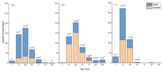
Figure 2.
Sex ratio of H. tibetana population at different age classes. (a) Low altitude; (b) middle altitude; (c) high altitude. * indicates the sex ratio deviate from 1:1 significantly at p < 0.05 level; ns indicates that it did not significantly deviate from 1:1 (p ≥ 0.05).
3.2. Spatial Distribution Pattern of H. tibetana Populations at Different Altitudes
3.2.1. Population Spatial Distribution Types and Spatial Correlation Analysis
The population at a low altitude was basically randomly distributed at different scales, and within a small scale (0.5–0.75 m) showed a slightly aggregated distribution. The middle-altitude population showed a random distribution on the scale of 0–1 m and aggregated distribution on a scale greater than 1 m. The high-altitude population showed a basically random distribution at different spatial scales (Figure 3).
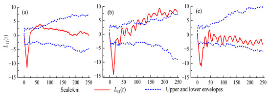
Figure 3.
Spatial distribution pattern of H. tibetana. (a) Low altitude; (b) middle altitude; (c) high altitude.
3.2.2. Spatial Correlation Between Male and Female Plants
A negative spatial correlation between the female and male individuals in the low-altitude population was observed (Figure 4a). In the middle-altitude population, female and male individuals showed a negative spatial correlation at small scales (0–0.5 m), and at larger scales (0.5–2.5 m), the correlation between female and male plants was not strong, indicating a spatial independence (Figure 4b).
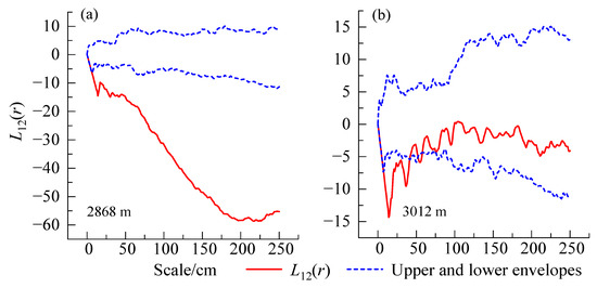
Figure 4.
Spatial association between female and male H. tibetana. (a) Low altitude; (b) middle altitude.
3.3. Clonal Structure and Clonal Diversity of H. tibetana
3.3.1. SSR Primer Amplification Results
PCR amplification was performed on 344 samples using 7 pairs of SSR primers obtained from the preliminary screening. The average observed heterozygosity Ho of H. tibetana at low and middle altitudes was 0.543. The expected heterozygosity He was 0.392, and the polymorphism information content PIC was 0.323 (in the Schedule 2 Polymorphism of SSR primers to H. tibetana (Figure 5), the amplification results of some primers to H. tibetana at different altitudes can be seen).
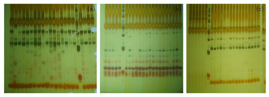
Figure 5.
Amplification results of some primers to H. tibetana at different altitudes. Amplification results of (a) Hr05 primer for middle-altitude individuals; (b) HTP-33 primer for low-altitude population; (c) HTP-35 primer for high-altitude population.
3.3.2. Identification of H. tibetana Clonal Genets
The NTSYS software was used to calculate the J&C genetic distance between individuals within the population, and identify individuals with a J&C genetic distance of 0 as the same genet. According to the clustering results of NTSYS, a total of 72 genets were identified from 190 individuals in the low-altitude population, and a total of 43 genets were identified from 154 individuals in the middle-altitude population.
3.3.3. Clonal Diversity of H. tibetana
There were differences in the clonal diversity index of populations at different altitudes (Table 2). The ratio of different genotypes (PD = 0.379) and Simpson diversity index (D = 0.973) of low-altitude populations were both greater than those in the middle-altitude populations. Moreover, the genotypic evenness of H. tibetana was also greater at low altitudes than at the middle altitude. According to Simpson diversity index (D), the clonal diversity of male groups at low and middle altitudes was greater than that of females. According to the different genotype ratios (PD) (Table 3), the clonal diversity of females at low altitudes was greater than that of males, and the opposite was true at the middle altitude. The genotype evenness (E) at low and middle altitudes showed that males were greater than females.
Table 2.
Clonal diversity of H. tibetana at different altitudes.
Table 3.
Clonal diversity of male and female H. tibetana.
3.4. Clone Size of H. tibetana
Both the low- and middle-altitude populations were composed of polyclones. Here, 72 genotypes (72 genets) were identified in 190 ramets in the low-altitude population, and each genet can produce between 1 and 17 ramets (Table 4). About 54.2% of the genets can produce more than 1 ramet, and each genet can produce 2.6 ramets on average. Among the 154 plants in the middle-altitude population, 43 plants had a clonal propagation ability. Each base plant can produce a number of ramets ranging from 1 to 20. The M-4, M-5, and M-6 genets can produce 15, 17, and 20 ramets, respectively, with an average clone size of 3.6 ramets per base plant. The average clone size in the middle-altitude population was larger than that in the low-altitude population.
Table 4.
Clone size of H. tibetana at different altitudes.
The 98 individuals in the low-altitude female population contained 36 genets, and each genet can produce an average of 2.7 ramets. About 45% of the genets only produced 1 ramet, and one genet can produce up to 17 ramets (Table 5). A total of 29 cloned genets were identified in the low-altitude male population. On average, each genet included 2.8 ramets and 55.2% of the genets can produce more than 1 ramet. One genet can produce up to fourteen ramets (Table 4); meanwhile, at a low altitude, there were nine ramets whose genders we failed to determine due to the fact that both they themselves and their adjacent ramets were too young. We have already marked this in Figure 6. The 57 ramets in the middle-altitude female population were cloned from 15 genets. On average, each genet can produce 3.8 ramets. Nearly half of the genets can produce more than one ramet. Twenty-eight different genotypes can be identified in the middle-altitude male population, with an average of 3.5 ramets per genet. Half of the genets can produce at least two ramets, and 1 genet can be cloned to produce up to 20 ramets (Table 6), which was lower than that of females. The average clone size was as follows: middle altitude > low altitude; middle altitude: female > male, low altitude: male > female.
Table 5.
Clone size of male and female H. tibetana at low altitude.
Table 6.
Clone size of male and female H. tibetana at middle altitude.
3.5. Clonal Distribution of H. tibetana Population
Clonal plants are affected by different environmental conditions and can expand in several directions at the same time according to the environmental conditions. The clonal distribution in the low- and middle-altitude populations is shown in Figure 6.
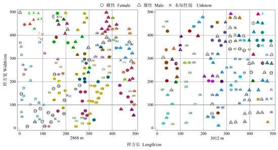
Figure 6.
Clonal distribution of H. tibetana (the same color in the same plot represents the same genotype).
The distances between the ramets in the same clone of H. tibetana female and male populations at different altitudes are shown in Table 7 and Table 8. The maximum distance (l max), minimum distance (l min), and total distance (L) between ramets in the same clone, and the average distance between ramets within a clone (M = L/N) were quantified.
Table 7.
Distance between ramets in the low-altitude population (m).
Table 8.
The distance between ramets at middle altitude (m).
At the low altitude, the maximum distance (l max) between two ramets in the same clone of the female population was 3.44 m, and the minimum distance was 0.12 m. The maximum total distance (L) between ramets in the same clone was 7.4 m. The average distance (M) between strains ranged from 0.06–1.56 m. At this altitude, the maximum distance between two ramets of the male group was 4.48 m, the minimum distance was 0.12 m, and the maximum total distance between ramets within the same clone was 7.56 m with an average distance (M) between two ramets ranging from 0.12–1.34 m. In the female population at the middle altitude, the maximum distance between two ramets in the same clone was 5.00 m, the minimum distance was 0.19 m, and the maximum total distance between all ramets in the same clone was 11.57 m. The average distance between two ramets was 0.26–1.34 m. The maximum and minimum distance between two ramets in the same clone of the male population at this altitude was 4.81 m and 0.19 m, respectively. The distance between all ramets in the same clone had a maximum total distance of 11.95 m. The maximum value of the average distance between two ramets was 1.08 m, and the minimum value was 0.20 m. According to the distance between two ramets within the same clone, the clonal expansion capacity of male plants at the low altitude was greater than that of female plants, while that of female plants at the middle altitude was greater than that of male plants. Based on the distance between ramets within the same clone and the total distance between plants, the clonal extension ability of plants at the middle altitude was higher than that of plants at the low altitude.
4. Discussion
4.1. Sex Ratio Pattern of H. tibetana Population at Different Altitudes
The sex ratio theory proposed that the female-to-male ratio should be 1:1 [41], but this can be altered by ecological and genetic factors, resulting in sex-biased ratios [42]. A study investigating the sex ratio of H. tibetana in the Wolong Mountains found that the population sex ratio of H. tibetana was balanced at the optimum altitude for growth (2800 m), while the sex ratio was male-biased at other altitudes [43]. In this study, the age class sex ratio of H. tibetana mainly consists of age classes II and III (Figure 2), which also determines the sex ratio bias of H. tibetana. The H. tibetana population exhibited the significant sex-biased ratios at the middle and low altitudes compared to the high altitude. The male-biased sex ratio (p < 0.05) at the low-altitude (2868 m) population may be because H. tibetana female is more inferior for nutritional growth than males due to their higher reproductive investment, and under nutrient-limited conditions, female plants had higher mortality rates, resulting in a male-biased sex ratio [44,45].
In contrast, at the middle altitude, H. tibetana showed a female-biased sex ratio (p < 0.05). This was not consistent with the higher mortality rate of females in H. tibetana in the face of a harsh environment such as cold and intense UV-B ultraviolet light stress. This may be related to the fact that the soil was less infertile at the middle altitude compared to the other two altitudes [20]; thus, in order to better adapt to the harsh environment, females may have adopted additional mechanisms to compensate for the investment in growth under poorer conditions to improve surviving [46]. For example, Fan et al. [20] found that at the middle altitude, H. tibetana females photosynthesized better than males and survived better than males. Moreover, it has been suggested that in wind-pollinated plants, the reproductive cost of males may exceed that of females because males invested more in nitrogen-rich pollen [47]. H. tibetana is a typical wind-borne plant, which explained why females could out-compete males under more severe environmental constraints at the middle altitude [47]. The above results suggested that the different sex ratio patterns were a manifestation of the different ways in which the male and female H. tibetana adapt to the various environments.
4.2. Sex-Related Spatial Distribution Patterns of H. tibetana
At low and high altitudes, the sex-related distribution was generally random, which may be caused by H. tibetana adopting extensive foraging in order to minimize the competition. However, at mid-altitude, the distribution showed an aggregated distribution as the scale increased, possibly due to the fact that the mid-altitude is more resource-poor, which leads to the adoption of intensity foraging in some patches [48].
Sexual dimorphism might influence the frequency and distribution of the sexes under different environmental conditions, likely resulting in the niche differentiation and spatial segregation of the sexes [7]. The spatial correlation of female and male populations of H. tibetana showed differences at different altitudes. There was a strong negative spatial correlation in the low-altitude (2868 m) populations, which indicated that the ecological niche overlap between female and male H. tibetana plants at low altitudes caused strong intraspecific competition [49]; meanwhile, the stronger clonal reproductive capacity and lower clonal expansion ability of males compared to females at a low altitude may exacerbate this point. Male and female populations at the middle-altitude (3012 m) site showed a negative spatial correlation at small scales (0–0.5 m), and basically showed no correlation as the scale increased. During the field survey, young individuals of H. tibetana exhibited the phenomenon of aggregated growth due to short horizontal roots. As the age increased, H. tibetana produced clonal ramets in different directions through spacers, coupled with its strong expansion ability, allowing it to occupy different habitats. Independent spaces for males and females form on a scale greater than 0.5 m. This distribution pattern showed that as the scale of the population at the middle altitude (3012 m) increased, the competition for resources and space between male and female plants weakened, and the stronger clonal reproductive and expansion abilities of females than those of males at the middle altitude may also play an important role in this regard. Individuals of different genders can thus occupy different microenvironments and make full use of resources. This was considered to be one of the evolutionary advantages of a dioecious plant [50]. These suggested that the sex-specific clonality of H. tibetana is able to better utilize its resources for the benefit of population development.
4.3. Sex-Related Clonal Diversity and Clonal Structure of H. tibetana
In this study, we found that the clonal diversity of H. tibetana varied across altitudes and between males and females. The clonal diversity at the middle altitude was lower than that at the low altitude. This was due to the fact that at the middle altitude, plant life is challenged by low temperatures, shorter vegetation periods, and harsher conditions Fan et al. [20] which may reduce sexual reproduction and increase inputs to asexual reproduction [51,52], thus leading to a decrease in clonal diversity. Moreover, the clonal diversity of H. tibetana was higher in males than in females at the middle altitude, which suggested that clonal reproduction played a more important role than sexual reproduction in females at the middle altitude [53]. Meanwhile, Wang et al. [23] showed that higher clonal diversity increased the evolutionary rate of adaptation to harsh alpine environments and, therefore, male plants were more dependent on clonal diversity for adaptation to nutrient-poor mid-altitude regions. These indicated that faced with different environments, the relative importance of sexual reproduction versus clonal reproduction of H. tibetana might change to better adapt to the environment.
The clone size and spacer length of H. tibetana also varied and showed similar trends, both of which were larger at the middle altitude than at the low altitude, and females were larger than males at the middle altitude, while the opposite was true at the low altitude, however, the spacer length of males is shorter. The above changes indicated that the cloning and expansion ability of H. tibetana were higher than that at the low altitude, and females were greater than males at the middle altitude. At the same time, differences in the spacer length also indicated that H. tibetana could break through the limitation of the resource distribution within a certain range by adapting its morphology, thus expanding its growing space. Since the above clonal variation in the morphology was also significant between males and females, and in combination with the differences in the spatial distribution of H. tibetana, we believe that the clonal variation between males and females of H. tibetana separated males and females from each other, which assisted in the distribution of H. tibetana population. Therefore, the differences in the clonal diversity and clonal structure between male and female H. tibetana were also the result of their long-term adaptation to the external environment.
It should be noted that our study has a limitation in terms of the population sampling. We only analyzed two populations spatially and genetically without replicates. This limited sampling may not fully represent the entire range of genetic and spatial variability within the species. The results obtained from these two populations may not be generalizable to all H. tibetana populations across different regions or habitats. Therefore, when interpreting our findings, caution should be exercised as the observed patterns and relationships might be specific to the sampled populations and not necessarily indicative of the overall species. Future studies with more extensive sampling are needed to confirm and expand on our results.
5. Conclusions
In summary, H. tibetana exhibits different sex-biased ratios at different altitudes, indicating that male and female H. tibetana respond differently to different environmental conditions. In addition, as a clonal plant, H. tibetana also adopts sex-specific reproductive modes in response to stressful environments, which is mainly manifested in the different clonal diversity and clonal reproductive capacity of female and male populations of H. tibetana. Also, the sex-differentiated distribution patterns and clone structure at different altitudes suggests that H. tibetana sex-specific differences are conducive to H. tibetana occupying different habitats and making full use of environmental resources. Therefore, sex-specific differences in the clonality of H. tibetana effectively improves the adaptation of the H. tibetana population to the environment, thus enhancing the survival and continuation of the H. tibetana population.
Author Contributions
B.F. designed this study, collected the data, wrote and revised the first draft, and led the writing on subsequent revisions. Y.W. and N.D. wrote the first draft and drew the figures. T.T. collected the data. B.F. and K.S. provided input regarding the study design of the manuscript. All authors have read and agreed to the published version of the manuscript.
Funding
This research was funded by the National Natural Science Foundation of China (32260271, 32460257), the Gansu province’s Key Research and Development Plan (21YF5NA069), the Longyuan Talent Youth Innovation and Entrepreneurship Team project (2022LQTD56), and the Foreign Expert Introduction Special Project of Gansu Province (22JR10KA010).
Data Availability Statement
The datasets used and analyzed during the current study are available from the corresponding author on reasonable request.
Acknowledgments
We sincerely thank Charles Hocart (The Australian National University) for his efforts in proof-reading our paper, and we thank Jing Lu for their dedicated assistance during the fieldwork and experiments in the lab.
Conflicts of Interest
The authors declare no conflicts of interest.
References
- Eckert, C.G.; Lui, K.; Bronson, K.; Corradini, P.; Bruneau, A. Population genetic consequences of extreme variation in sexual and clonal reproduction in an aquatic plant. Mol. Ecol. 2003, 12, 331–344. [Google Scholar] [CrossRef]
- Albert, T.; Raspé, O.; Jacquemart, A.L. Clonal Diversity and Genetic Structure in Vaccinium myrtillus Populations from Different Habitats. Belg. J. Bot. 2004, 137, 155–162. Available online: http://www.jstor.org/stable/20794549 (accessed on 26 December 2023).
- Ren, M.X.; Zhang, Q.G. Clonal diversity and structure of the invasive aquatic plant Eichhornia crassipes in China. Aquat. Bot. 2007, 87, 242–246. [Google Scholar] [CrossRef]
- Bachmann, K. Molecular markers in plant ecology. New Phytol. 1994, 126, 403–418. [Google Scholar] [CrossRef]
- Barrett, S.C.; Yakimowski, S.B.; Field, D.L.; Pickup, M. Ecological genetics of sex ratios in plant populations. Philos. Trans. R. Soc. Lond. B Biol. Sci. 2010, 27, 2549–2557. [Google Scholar] [CrossRef] [PubMed]
- Alberto, F.; Gouveia, L.; Arnaud-Haond, S.; Pérez-Lloréns, J.L.; Duarte, C.M.; Serrão, E.A. Within-population spatial genetic structure, neighbourhood size and clonal subrange in the seagrass Cymodocea nodosa. Mol. Ecol. 2005, 14, 2669–2681. [Google Scholar] [CrossRef]
- Liu, M.; Korpelainen, H.; Li, C. Sexual differences and sex ratios of dioecious plants under stressful environments. J. Plant Ecol. 2021, 14, 920–933. [Google Scholar] [CrossRef]
- Garbarino, M.; Weisberg, P.J.; Bagnara, L.; Urbinati, C. Sex-related spatial segregation along environmental gradients in the dioecious conifer, Taxus baccata. For. Ecol. Manag. 2015, 358, 122–129. [Google Scholar] [CrossRef]
- Barrett, S.C.; Hough, J. Sexual dimorphism in flowering plants. J. Exp. Bot. 2013, 64, 67–82. [Google Scholar] [CrossRef]
- Sinclair, J.P.; Emlen, J.; Freeman, D.C. Biased Sex Ratios in Plants: Theory and Trends. Bot. Rev. 2012, 78, 63–86. [Google Scholar] [CrossRef]
- Munné-Bosch, S. Sex ratios in dioecious plants in the framework of global change. Environ. Exp. Bot. 2015, 109, 99–102. [Google Scholar] [CrossRef]
- Juvany, M.; Munné-Bosch, S. Sex-related differences in stress tolerance in dioecious plants: A critical appraisal in a physiological context. J. Exp. Bot. 2015, 66, 6083–6092. [Google Scholar] [CrossRef]
- Petry, W.K.; Soule, J.D.; Iler, A.M.; Chicas-Mosier, A.; Inouye, D.W.; Miller, T.E.; Mooney, K.A. Sex-specific responses to climate change in plants alter population sex ratio and performance. Science 2016, 353, 69–71. [Google Scholar] [CrossRef]
- Condit, R.; Ashton, P.S.; Baker, P.; Bunyavejchewin, S.; Gunatilleke, S.; Gunatilleke, N.; Hubbell, S.P.; Foster, R.B.; Itoh, A.; LaFrankie, J.V.; et al. Spatial patterns in the distribution of tropical tree species. Science 2000, 288, 1414–1418. [Google Scholar] [CrossRef]
- Fibich, P.; Lepš, J.; Novotný, V.; Klimeš, P.; Těšitel, J.; Molem, K.; Damas, K.; Weiblen, G.D. Spatial patterns of tree species distribution in New Guinea primary and secondary lowland rain forest. J. Veg. Sci. 2016, 27, 328–339. [Google Scholar] [CrossRef]
- Lian, Y.S.; Chen, X.L.; Lian, H. Systematic classification of the genus hippophae L. Seabuckthorn. Res. 1998, 1, 13–23. [Google Scholar]
- Kalia, R.K.; Singh, R.; Rai, M.K.; Mishra, G.P.; Singh, S.R.; Dhawan, A.K. Biotechnological interventions in sea buckthorn (Hippophae L.): Current status and future prospects. Trees 2011, 25, 559–575. [Google Scholar] [CrossRef]
- Wang, R.; Wu, B.; Jian, J.; Tang, Y.; Zhang, T.; Song, Z.; Zhang, W.; Qiong, L. How to survive in the world’s third poplar: Insights from the genome of the highest altitude woody plant, Hippophae tibetana (Elaeagnaceae). Front. Plant Sci. 2022, 13, 1051587. [Google Scholar] [CrossRef]
- Körner, C. Alpine Plant Life: Functional Plant Ecology of High Mountain Ecosystems; Springer: Berlin/Heidelberg, Germany, 2003. [Google Scholar]
- Fan, B.; Ma, Z.; Gao, P.; Lu, J.; Ding, N.; Sun, K. Functional Traits of Male and Female Leaves of Hippophae tibetana on the Eastern Edge of the Tibetan Plateau and Their Altitudinal Variability. Plants 2022, 11, 2484. [Google Scholar] [CrossRef]
- Lu, C.; Shan, Y.; Liu, H.; Yang, L.; Ma, G. Natural vitamin king seabuckthorn in the application of food ingredients. China. Food. Addit. 2008, S1, 230–235. [Google Scholar]
- Lei, Y.; Jiang, Y.; Chen, K.; Duan, B.; Zhang, S.; Korpelainen, H.; Niinemets, Ü.; Li, C. Reproductive investments driven by sex and altitude in sympatric Populus and Salix trees. Tree Physiol. 2017, 37, 1503–1514. [Google Scholar] [CrossRef] [PubMed]
- Wang, X.; Zhao, W.; Li, L.; You, J.; Ni, B.; Chen, X. Clonal plasticity and diversity facilitates the adaptation of Rhododendron aureum Georgi to alpine environment. PLoS ONE 2018, 13, e0197089. [Google Scholar] [CrossRef]
- Klimešová, J.; Doležal, J. Are clonal plants more frequent in cold environments than elsewhere? Plant Ecol. Divers. 2011, 4, 373–378. [Google Scholar] [CrossRef]
- Miao, F.H.; Guo, Y.J.; Miao, P.F.; Guo, Z.G.; Shen, Y.Y. Influence of enclosure on community characteristics of alpine meadow in the northeastern edge region of the Qinghai-Tibetan plateau. Acta Prataculturae Sin. 2012, 21, 11. (In Chinese) [Google Scholar]
- Allen, G.A.; Antos, J.A. Sex ratio variation in the dioecious shrub Oemleria cerasiformis. Am. Nat. 1993, 141, 537–553. [Google Scholar] [CrossRef] [PubMed]
- Su, Z.; Zhou, X.; Zhou, L.; Jiang, X.; Kang, X. Population structure and dynamics of an endangered desert shrub endemic to Northwestern China. Pak. J. Bot. 2021, 53, 1361–1370. [Google Scholar] [CrossRef] [PubMed]
- Ripley, B.D. Modelling spatial patterns. J. R. Stat. Soc. Ser. B (Methodol.) 1977, 39, 172–192. [Google Scholar] [CrossRef]
- Besag, J. Contribution to the discussion of Dr. Ripley’ s paper. J. R. Stat. Soc. Ser. B (Methodol.) 1977, 39, 193–195. [Google Scholar]
- Lotwick, H.W.; Silverman, B.W. Methods for Analysing Spatial Processes of Several Types of Points. Journal of the royal statistical society series. Transp. Res. B-Meth 1982, 44, 406–413. [Google Scholar] [CrossRef]
- Diggle, P.J. Statistical Analysis of Spatial Point Patterns; Academic Press: New York, NY, USA, 1983. [Google Scholar]
- Zhang, L.; Gao, Y.; Li, J.; Zhang, C.; Li, M.; Hu, Z.; Cui, X. Effects of grazing disturbance of spatial distribution pattern and interspecies relationship of two desert shrubs. J. For. Res. 2021, 33, 507–518. [Google Scholar] [CrossRef]
- Doyle, J.J.A. A rapid DNA isolation procedure for small quantities of fresh leaf tissue. Phytochem. Bull. 1987, 19, 11–15. [Google Scholar]
- Wang, A.; Zhang, Q.; Wan, D.; Yang, Y.; Liu, J. Nine microsatellite DNA primers for Hippophae rhamnoides ssp. sinensis (Elaeagnaceae). Conserv. Genet. 2008, 9, 969–971. [Google Scholar] [CrossRef]
- Taberlet, P.; Gielly, L.; Pautou, G.; Bouvet, J. Universal primers for amplification of three non-coding regions of chloroplast DNA. Plant Mol. Biol. 1991, 17, 1105–1109. [Google Scholar] [CrossRef] [PubMed]
- Xu, T.; Xu, L.; Wang, H.; La, Q.; Sun, K.; Zhang, W. Development of Polymorphic Microsatellite Markers from Hippophae tibetana Using 5′-Anchored PCR Methods and Magnetic Beads Hybridization. J. Fudan Univ. 2014, 53, 543–549. [Google Scholar]
- Marshall, T.C.; Slate, J.; Kruuk, L.E.; Pemberton, J.M. Statistical confidence for likelihood-based paternity inference in natural populations. Mol. Ecol. 1998, 7, 639–655. [Google Scholar] [CrossRef] [PubMed]
- Hill, M.O.; Pielou, E.G. An introduction to mathematical ecology. J. Ecol. 1970, 58, 896. [Google Scholar] [CrossRef]
- Fager, E.W. Diversity: A Sampling Study. Am. Nat. 1972, 106, 293–310. [Google Scholar] [CrossRef]
- Parker, E.D. Ecological Implications of Clonal Diversity in Parthenogenetic Morphospecies. Am. Zool. 1979, 19, 753–762. [Google Scholar] [CrossRef]
- Field, D.L.; Pickup, M.; Barrett, S.C. Comparative analyses of sex-ratio variation in dioecious flowering plants. Evolution 2013, 67, 661–672. [Google Scholar] [CrossRef] [PubMed]
- Decker, K.L.; Pilson, D. Biased sex ratios in the dioecious annual Croton texensis (Euphorbiaceae) are not due to environmental sex determination. Am. J. Bot. 2000, 87, 221–229. [Google Scholar] [CrossRef]
- Li, C.; Xu, G.; Zang, R.; Korpelainen, H.; Berninger, F. Sex-related differences in leaf morphological and physiological responses in Hippophae rhamnoides along an altitudinal gradient. Tree Physiol. 2007, 27, 399–406. [Google Scholar] [CrossRef] [PubMed]
- Delph, L.F. Sexual dimorphism in life history. In Gender and Sexual Dimorphism in Flowering Plants; Springer: Berlin/Heidelberg, Germany, 1999; pp. 149–173. [Google Scholar]
- Rocheleau, A.F.; Houle, G. Different cost of reproduction for the males and females of the rare dioecious shrub Corema conradii (Empetraceae). Am. J. Bot. 2001, 88, 659–666. [Google Scholar] [CrossRef] [PubMed]
- Jiang, H.; Zhang, S.; Lei, Y.; Xu, G.; Zhang, D. Alternative Growth and Defensive Strategies Reveal Potential and Gender Specific Trade-Offs in Dioecious Plants Salix paraplesia to Nutrient Availability. Front. Plant Sci. 2016, 20, 1064. [Google Scholar] [CrossRef] [PubMed]
- Harris, M.S.; Pannell, J.R. Roots, shoots and reproduction: Sexual dimorphism in size and costs of reproductive allocation in an annual herb. Proc. Biol. Sci. 2008, 22, 2595–2602. [Google Scholar] [CrossRef]
- Slade, A.J.; Hutchings, M.J. The effects of nutrient availability on foraging in the clonal herb Glechoma hederacea. J. Ecol. 1987, 78, 95–112. [Google Scholar] [CrossRef]
- Wiegand, T.; Moloney, K.A. Rings, circles, and null-models for point pattern analysis in ecology. Oikos 2004, 104, 209–229. [Google Scholar] [CrossRef]
- Matsushita, M.; Takao, M.; Makita, A. Sex-different response in growth traits to resource heterogeneity explains male-biased sex ratio. Acta Oecologica 2016, 75, 8–14. [Google Scholar] [CrossRef]
- Eriksson, O. Clonal life histories and the evolution of seed recruitment. In The Ecology and Evolution of Clonal Plants; Backhuys Publishers: Leiden, The Netherlands, 1997; pp. 211–226. [Google Scholar]
- Verburg, R.; Grava, D. Differences in allocation patterns in clonal and sexual offspring in a woodland pseudo-annual. Oecologia 1998, 115, 472–477. [Google Scholar] [CrossRef]
- Kreher, S.A.; Fore, S.A.; Collins, B.S. Genetic variation within and among patches of the clonal species, Vaccinium stamineum L. Mol. Ecol. 2000, 9, 1247–1252. [Google Scholar] [CrossRef] [PubMed]
Disclaimer/Publisher’s Note: The statements, opinions and data contained in all publications are solely those of the individual author(s) and contributor(s) and not of MDPI and/or the editor(s). MDPI and/or the editor(s) disclaim responsibility for any injury to people or property resulting from any ideas, methods, instructions or products referred to in the content. |
© 2025 by the authors. Licensee MDPI, Basel, Switzerland. This article is an open access article distributed under the terms and conditions of the Creative Commons Attribution (CC BY) license (https://creativecommons.org/licenses/by/4.0/).