Figure 1.
The Scolytidae forestry pest data. (a) natural light, no alcohol, crowded, (b) hit light, no alcohol, sparse.
Figure 1.
The Scolytidae forestry pest data. (a) natural light, no alcohol, crowded, (b) hit light, no alcohol, sparse.
Figure 2.
Sample IP102 dataset. (a) Field Crop pests and (b) economic crop pests.
Figure 2.
Sample IP102 dataset. (a) Field Crop pests and (b) economic crop pests.
Figure 3.
Classification of the IP102 dataset. “FC” and “EC” denote Field Crops and Economy Crops. At the subclass level in the figure, only 33 subclasses are shown.
Figure 3.
Classification of the IP102 dataset. “FC” and “EC” denote Field Crops and Economy Crops. At the subclass level in the figure, only 33 subclasses are shown.
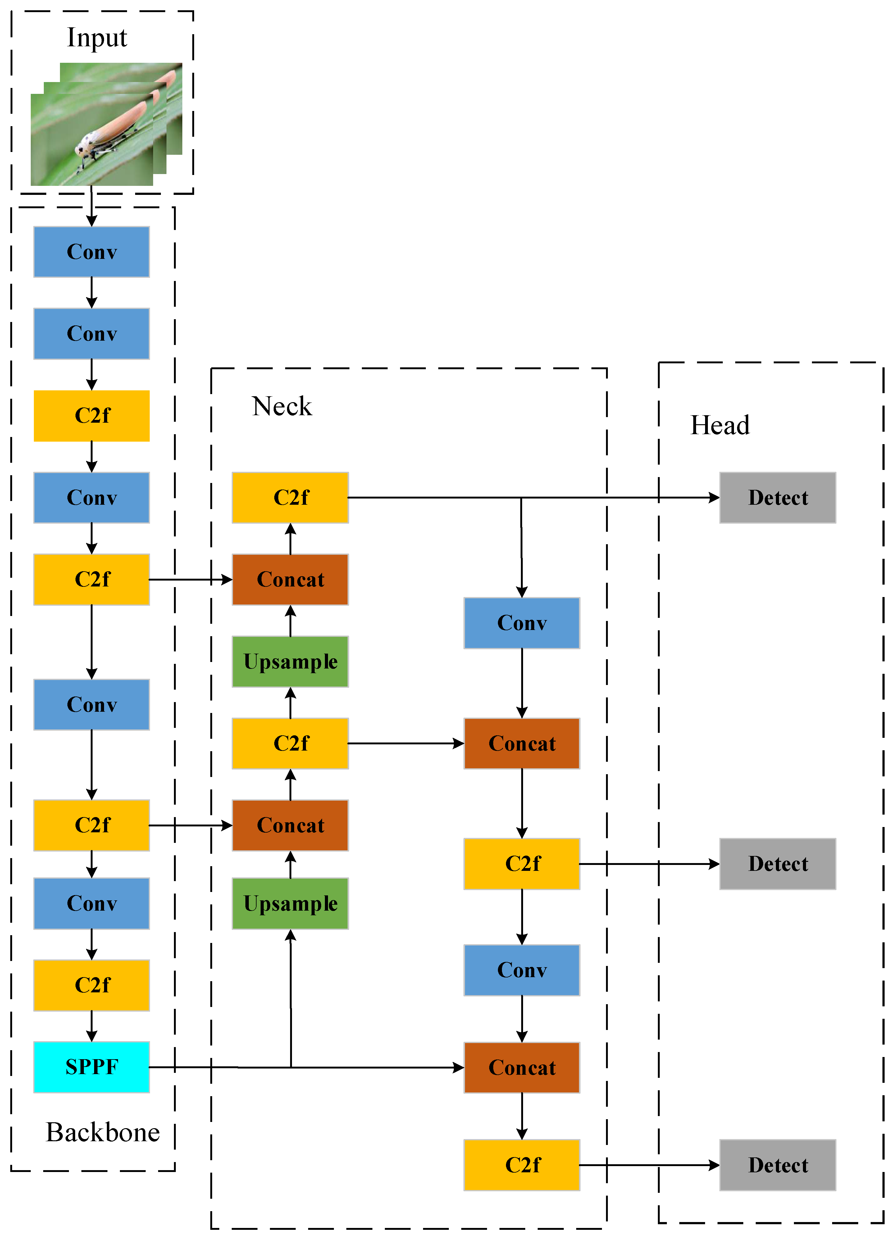
Figure 4.
YOLOv8 model structure.
Figure 4.
YOLOv8 model structure.
Figure 5.
GLU-YOLOv8 model structure.
Figure 5.
GLU-YOLOv8 model structure.
Figure 6.
Calculation of the SIOU loss function.
Figure 6.
Calculation of the SIOU loss function.
Figure 7.
CBAM Attention Structure.
Figure 7.
CBAM Attention Structure.
Figure 8.
LSK attention structure.
Figure 8.
LSK attention structure.
Figure 9.
EMA Attention Structure.
Figure 9.
EMA Attention Structure.
Figure 10.
GLU-CONV convolutional block structure.
Figure 10.
GLU-CONV convolutional block structure.
Figure 11.
Activation Function. GELU is smooth near zero, which benefits the gradient continuity and flow. In contrast, RELU is nondifferentiable at zero, potentially causing instability during optimization. Tanh and Sigmoid have sharply diminishing gradients near their extremities, which can also lead to inefficient optimization. The non-saturation and smoothing nature of GELU make it easier to avoid the problem of vanishing or exploding gradients during training, and helps the model converge faster.
Figure 12.
Improved Neck structural form. The numbers in the figure indicate the number of layers in which the module is located, where Detect is the last detection layer.
Figure 12.
Improved Neck structural form. The numbers in the figure indicate the number of layers in which the module is located, where Detect is the last detection layer.
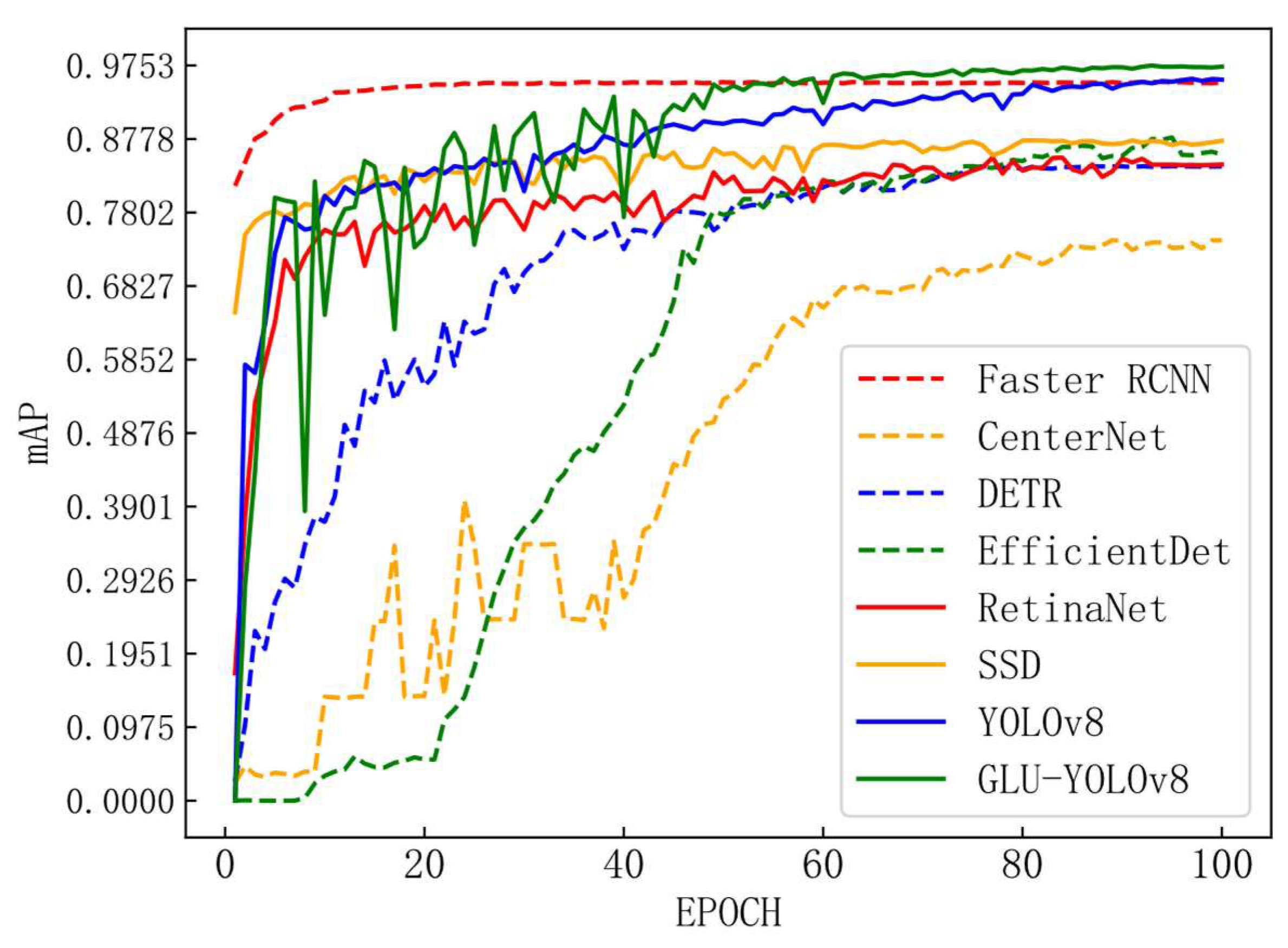
Figure 13.
mAP, and iteration number variation chart.
Figure 13.
mAP, and iteration number variation chart.
Figure 14.
Detection plots for the ablation experiment. Two representative photos (a,b) in the dataset exhibit different light sources and sparse conditions. Thermogram photos (c), (e), and (d), (f) correspond to (a) and (b), respectively. Thermograms (c,d) belong to the original YOLOv8 model, while (e,f) belong to the GLU-YOLOv8 model. The comparison reveals that the model proposed in this paper places greater emphasis on the lower body of the pest during decision-making. Moreover, the model demonstrates a more focused ability to extract features of the pest’s trunk compared to the original YOLOv8 model, which prioritizes detailed features of the lower limbs.
Figure 15.
mAP, and iteration number variation chart.
Figure 15.
mAP, and iteration number variation chart.
Figure 16.
GLU-YOLOv8 model confusion matrix. The model effectively identifies six types of pests with excellent overall performance. However, it shows a slight weakness in distinguishing between Coleoptera and Acuminatus, leading to potential misjudgment. In contrast, the model excels in identifying the remaining four types of pests. Future work should focus on addressing these shortcomings and enhancing the model’s ability to differentiate between Coleoptera and Acuminatus.
Figure 17.
IP102 dataset detection map.
Figure 17.
IP102 dataset detection map.
Figure 18.
Loss and iteration number variation chart.
Figure 18.
Loss and iteration number variation chart.
Figure 19.
The heat map. (a) shows the original image, (b) shows the recognition heat map of the YOLOv8 model, (c) shows the recognition heat map of the GLU-YOLOv8 model. A comparison between (b,c) reveals that the red area in (c) is more intense and concentrated, indicating that the model proposed in this study exhibits enhanced focus and stronger feature extraction capabilities.
Figure 20.
The histogram of model classification results. The GLU-YOLOv8 model excels in image classification, particularly in terms of high accuracy and overall performance. Compared to the other models, GLU-YOLOv8 demonstrates the highest accuracy, surpassing the performance of the comparison models. Additionally, GLU-YOLOv8 remains competitive in precision, recall, and F1 metrics, showcasing a balanced performance across various dimensions.
Table 1.
Statistics of insect instances in the Scolytidae forestry dataset.
Table 1.
Statistics of insect instances in the Scolytidae forestry dataset.
| Name | Number | Train | Test |
|---|
| Leconte | 2711 | 2493 | 218 |
| Boerner | 1859 | 1682 | 177 |
| Linnaeus | 1953 | 1759 | 194 |
| Armandi | 1932 | 1737 | 195 |
| Coleoptera | 2163 | 1934 | 229 |
| Acuminatus | 1130 | 1021 | 109 |
Table 2.
Number of samples in the IP102 dataset.
Table 2.
Number of samples in the IP102 dataset.
| Superclass | Class | Train | Test | IR |
|---|
| FC | Rice | 14 | 5043 | 3374 | 1.5 |
| FC | Corn | 13 | 8404 | 5611 | 1.5 |
| FC | Wheat | 9 | 2048 | 1370 | 1.5 |
| FC | Beet | 8 | 2649 | 1771 | 1.5 |
| FC | Alfalfa | 13 | 6230 | 4160 | 1.5 |
| EC | Vitis | 16 | 10,525 | 7026 | 1.5 |
| EC | Citrus | 19 | 4356 | 2917 | 1.5 |
| EC | Mango | 10 | 5840 | 3898 | 1.5 |
| IP102 | FC | 57 | 24,374 | 16,286 | 1.5 |
| EC | 45 | 20,721 | 13,841 | 1.5 |
| IP102 | 102 | 45,095 | 30,127 | 1.5 |
Table 3.
Experimental parameter settings.
Table 3.
Experimental parameter settings.
| Parameter | Value | Parameter | Value |
|---|
| EPOCH | 100 | Input size | 640 × 640 |
| Initial learning | 0.01 | Momentum | 0.9 |
| Learning rate decay rate | 0.5 | Weight decay | 0.0001 |
| Learning rate decay period | 10 | Optimizer | SGD |
Table 4.
Structure of the ablation experiment model.
Table 4.
Structure of the ablation experiment model.
| Model | SIOU | CBAM | GLU-CONV | LSK | SODL |
|---|
| YOLOv8 | × | × | × | × | × |
| Model A | √ | × | × | × | × |
| Model B | √ | √ | × | × | × |
| Model C | √ | √ | √ | × | × |
| Model D | √ | √ | √ | √ | × |
| GLU-YOLOv8 | √ | √ | √ | √ | √ |
Table 5.
Ablation experiment model detection results.
Table 5.
Ablation experiment model detection results.
| Model | mAP@0.50 | mAP@0.50
(Area = Small) | mAP@0.5:0.95 | Precision | Recall | F1 | FPS |
|---|
| YOLOv8 | 95.7% | 83.2% | 74.9% | 91.2% | 91.2% | 0.911 | 20.34 |
| Model A | 95.8% | 83.4% | 74.8% | 91.1% | 91.0% | 0.905 | 20.12 |
| Model B | 96.1% | 84.3% | 77.1% | 92.8% | 91.6% | 0.920 | 29.07 |
| Model C | 96.9% | 85.6% | 78.9% | 94.9% | 94.0% | 0.944 | 18.72 |
| Model D | 97.1% | 86.3% | 78.5% | 94.5% | 94.8% | 0.946 | 17.92 |
| GLU-YOLOv8 | 97.4% | 91.6% | 81.2% | 95.8% | 94.1% | 0.949 | 17.24 |
Table 6.
Comparison of experimental model detection results.
Table 6.
Comparison of experimental model detection results.
| Model | mAP@0.50 | Precision | Recall | F1 | FPS |
|---|
| Faster RCNN | 95.2% | 87.1% | 78.3% | 0.823 | 4.54 |
| CenterNet | 74.4% | 91.7% | 79.9% | 0.695 | 12.34 |
| DETR | 84.2% | 79.1% | 88.7% | 0.830 | 21.43 |
| EfficientDet | 89.1% | 97.2% | 76.2% | 0.813 | 24.32 |
| RetinaNet | 85.3% | 91.7% | 78.5% | 0.845 | 8.73 |
| SSD | 87.5% | 77.7% | 73.7% | 0.756 | 11.45 |
| YOLOv8 | 95.8% | 91.1% | 91.0% | 0.905 | 20.12 |
| GLU-YOLOv8 | 97.4% | 95.8% | 94.1% | 0.949 | 17.24 |
Table 7.
Experimental model detection results.
Table 7.
Experimental model detection results.
| Model | mAP@0.50 | mAP@0.50:0.95 | Precision | Recall | F1 | FPS |
|---|
| Faster RCNN | 49.2% | 26.7% | 41.5% | 44.6% | 0.430 | 4.74 |
| CenterNet | 51.0% | 30.5% | 32.0% | 44.7% | 0.375 | 12.12 |
| DETR | 34.9% | 21.1% | 22.8% | 39.3% | 0.287 | 20.47 |
| EfficientDet | 54.9% | 30.3% | 52.8% | 50.7% | 0.517 | 22.45 |
| RetinaNet | 56.6% | 34.3% | 37.3% | 47.9% | 0.419 | 7.23 |
| SSD | 44.7% | 25.6% | 43.0% | 44.9% | 0.439 | 11.45 |
| YOLOv8 | 51.6% | 32.9% | 46.2% | 56.7% | 0.509 | 19.34 |
| GLU-YOLOv8 | 58.7% | 37.9% | 56.3% | 59.3% | 0.577 | 17.98 |
Table 8.
Comparison of experimental model classification results.
Table 8.
Comparison of experimental model classification results.
| Model | Accuracy (Top1) | Accuracy (Top5) | FPS |
|---|
| ResNet | 60.1% | 81.1% | 110.66 |
| SqueezeNet | 50.0% | 75.2% | 65.49 |
| ShuffleNetV2 | 63.9% | 84.4% | 97.87 |
| MobileNetV3 | 62.9% | 83.0% | 56.97 |
| ManasNet | 65.6% | 84.6% | 58.82 |
| GhostNet | 60.1% | 81.9% | 45.77 |
| EfficientNetV2 | 60.9% | 81.3% | 55.76 |
| ConvMixer | 60.8% | 81.0% | 82.20 |
| DPN | 61.4% | 81.6% | 84.33 |
| YOLOv8 | 63.5% | 86.6% | 243.90 |
| GLU-YOLOv8 | 66.9% | 88.0% | 126.58 |


