Abstract
The evaluation of site quality for mixed forests is a comprehensive approach to analyzing forest site conditions and tree species growth performance. Accurate site quality assessment is crucial for understanding and enhancing the ecological functions and productivity potential of forests. This study focuses on mixed forests in Lishui City, Zhejiang Province. Using the Two-way Indicator Species Analysis (TWINSPAN) method, coniferous mixed forest, broadleaved mixed forest, and mixed coniferous–broadleaved forests in the region were classified into 15 forest types. Site form models for each type were then constructed using the Algebraic Difference Approach (ADA) to categorize site quality levels. Subsequently, a site quality classification model was developed by integrating site and climatic factors, employing four machine learning algorithms: Random Forest (RF), K-Nearest Neighbors (KNN), Support Vector Machine (SVM), and XGBoost. This model effectively facilitated the evaluation of site quality in mixed forests. The results showed that, across the 15 forest types, the site form models based on the ADA method achieved R2 values greater than 0.634, indicating accuracy in capturing tree height growth trends in mixed forests. For site quality classification, all four models (RF, KNN, SVM, and XGBoost) achieved overall accuracies above 0.77. Among these, the machine learning models ranked in effectiveness for site quality classification as follows: XGBoost > RF > SVM > KNN. These findings suggest that the site form model is a suitable criterion for classifying site quality in mixed forests in Lishui City, Zhejiang Province, and that the XGBoost-based model demonstrates strong classification accuracy. This study provides a scientific basis for site-adapted tree selection and advances information on mixed forest management.
1. Introduction
Site quality refers to the production potential of a specific forest or vegetation type on a given site [1]. Forest quality and yield are closely related to site quality. Accurately and scientifically assessing forest site quality to fully realize the multifunctional value of forests has become a primary focus in forestry research [2,3,4]. Current site quality evaluations for even-aged pure forests are relatively well-established. Due to their uniform species composition and known planting times, the site quality of even-aged pure forests is typically evaluated using the site index based on the relationship between dominant height and age [5,6]. In contrast, the growth processes of mixed forests are more complex than those of even-aged forests. Their diverse species and age structures create significant challenges for site quality assessment. Establishing a precise and scientific evaluation system for mixed forest site quality could profoundly impact mixed forest management and sustainable development.
For the evaluation of site quality for mixed forests, some scholars have employed the biomass potential productivity method [7]. Others have utilized the growth index method to assess forest quality [8]. Additionally, some researchers have applied the site index method to evaluate the site quality of mixed forests. Lou et al. [9] utilized age–height data from natural secondary mixed forests of Juglans mandshurica (Juglans spp.) in Changbai Mountain, Jilin Province, to establish a polymorphic site index model. This model, based on univariate site index guiding curves for different site types, accurately reflects height growth differences across various site types for Juglans mandshurica. Ercanli et al. [10] developed a dynamic site index model for mixed forests of Scots pine (Pinus sylvestris L.) and Oriental beech (Fagus orientalis Lipsky) in northwestern Turkey based on stem analysis data from 397 dominant trees. Their study found that models based on the Bertalanffy–Richards and Hossfeld functions performed best in predicting dominant tree height. The site index method and its dynamic variant are widely used for assessing site productivity in mixed forests due to their simplicity and practical applicability. However, traditional site index models rely heavily on age-specific parameters, which limits their flexibility in forests with diverse species compositions and complex structures. Dynamic site index models improve upon this by incorporating temporal changes in stand development, but they often require extensive data and remain less adaptable to mixed-species conditions. Although the site index is commonly used for assessing forest productivity, its reliance on a reference age poses a significant limitation, particularly under the uneven-aged and complex growth conditions of mixed forests. Additionally, calculating the site index requires obtaining the age information of sample trees, which is both time-consuming and prone to inaccuracies in uneven-aged mixed forests. In contrast, the site form method, which is based on the relationship between tree diameter at breast height (DBH) and height, overcomes the dependence on age data and is better suited for evaluating site quality in complex forest ecosystems [11,12].
In the study of site form, Vanclay and Henry [11] were the first to propose “site form” as a method for evaluating productivity in uneven-aged forests, applying this approach to uneven-aged Araucaria-dominated coniferous forests(Araucaria cunninghamii Aiton ex D. Don) in Queensland, Australia. Herrera-Fernández et al. demonstrated that the site form method effectively assesses site quality in broadleaved forests within Neotropical secondary rainforests, showing that site form indicators provide valuable information on forest productivity and growth potential. This information is crucial for forest management and conservation across diverse environmental conditions [13]. For tropical humid forests, site form has been shown to be a key indicator when assessing productivity. Do et al. [14] used site form to indirectly estimate potential productivity in natural secondary tropical humid forests, confirming its effectiveness in this environment. The significance of this method lies in its ability to provide reliable data on site quality, aiding in the development of precise forest management and conservation strategies. Castano-Santamaría et al. [15] applied site form models to natural beech forests in northwestern Spain, using fitted dynamic equations to estimate site quality. Their findings revealed a significant correlation between site form and site index, demonstrating that site form effectively reflects site quality. Gao et al. [12] developed a site quality classification model for Chinese fir (Cunninghamia lanceolata (Lamb.) Hook.) plantations using both site index and site form models, concluding that the site form model provided more accurate assessments than the site index model. In summary, current research suggests that the relationship between diameter at breast height (DBH) and tree height is more closely associated with growth than age, and DBH is simpler, more convenient, and more accurate to measure. Consequently, site form is widely used in evaluating site quality for mixed or natural forests.
The construction of site quality models aims to enhance the classification of forest site quality. Given that the growth of mixed forest stands is a complex process influenced by factors such as time, site conditions, and climate, effective site classification generally requires investigating various influencing factors and assessing site conditions based on their differences. There are two main approaches to site quality classification. The first involves combining ecological, botanical, and geoscience characteristics, using expert judgment to classify forest sites. For instance, Barnes [16] explored ecological methods for ecosystem classification, with a particular focus on multi-factor site classification that incorporates factors like soil and climate. Tesch [17] emphasized that climate, soil, and hydrology are critical site factors affecting tree growth, and he advocated for an interdisciplinary approach—integrating geography and soil science—for forest site classification and evaluation. The second approach involves developing site quality classification models based on statistical methods. For example, Zhang et al. [18] applied quantitative theory to classify Eucalyptus urophylla (Eucalyptus urophylla S.T. Blake) plantations in Hainan Island and Leizhou Peninsula into 12 site types. Lu et al. [19] examined the relationship between dominant tree growth characteristics and site factors using quantitative theory, employing hierarchical clustering and canonical correlation analysis to classify and evaluate the growth potential of hybrid Eucalyptus (Eucalyptus spp.) plantations. Additionally, Zhang et al. [20] used dominant factor analysis to identify key factors and developed a site index table to assess site quality. However, these traditional site quality classification methods typically rely on multivariate statistical models. Since tree growth and site factors often exhibit complex nonlinear relationships, traditional linear or simple nonlinear models rely on oversimplified assumptions, limiting their effectiveness. With advances in computing, machine learning algorithms now offer a powerful alternative capable of handling high-dimensional data with complex nonlinear interactions, thus providing robust support for forest site quality classification and assessment [21]. Recent studies have highlighted the significant advantages of machine learning algorithms, such as Random Forest and Support Vector Machines, in estimating forest parameters and conducting large-scale forest quality assessments [22]. Moreover, machine learning techniques have been successfully applied to predict forest yields, further demonstrating their potential and versatility in forest quality evaluation [23]. Additionally, machine learning has shown promising results in utilizing site quality classification in plantations. For instance, Piri-Sahragard et al. [24] employed random forest to examine the relationship between site factors and the distribution of five plant species, including Haloxylon persicum (Persian saxaul), demonstrating that machine learning models outperform traditional mathematical modeling in evaluating site quality. Chen et al. [25] used decision tree algorithms to construct a site quality classification model for Chinese fir plantations in Jinping County, Guizhou Province, based on site factors selected through expert judgment, verifying growth patterns for Chinese fir. Most existing studies use a single machine learning algorithm for model construction without comparing multiple algorithms, and applications of machine learning for site quality classification in mixed forests remain rare.
To accurately assess forest quality on a specific site, it is essential to clarify the criteria for forest stand type classification and understand the relationship between site conditions and stand growth. Therefore, it is necessary to classify mixed forests based on these criteria. In this study, mixed forests in southwestern Zhejiang were selected as the research focus. Using the Two-way Indicator Species Analysis (TWINSPAN) method, the mixed forests were classified into different stand types. An Algebraic Difference Approach (ADA) was then applied to develop a site form model. On this basis, site and climatic factors were comprehensively considered to construct site quality classification models for mixed forests, utilizing four machine learning algorithms: Random Forest (RF), K-Nearest Neighbors (KNN), Support Vector Machine (SVM), and XGBoost. Through comparative analysis, the most suitable classification model for site quality was selected for each stand type. This research provides a more scientific and effective method for evaluating site quality in mixed forests, offering theoretical and technical support for forest land-use planning in Lishui City’s mixed forests.
2. Materials and Methods
2.1. Study Area
The study area is located in Lishui City, in southwestern Zhejiang Province (Figure 1). As of 2020, Lishui’s forested area covers 1.42 million ha, with a high forest coverage rate of 82.27% and a total standing volume of 96 million m3. The region experiences a subtropical monsoon climate, with an annual average temperature ranging from 18.2 °C to 19.6 °C, a frost-free period of 246–274 days, and annual precipitation days of between 54 and 186. The annual rainfall ranges from 1309.9 to 1970.5 mm, with annual sunlight hours of 1102.3 to 1759.6 h and a total annual radiation of 102.1 to 110.0 kWh/m2.
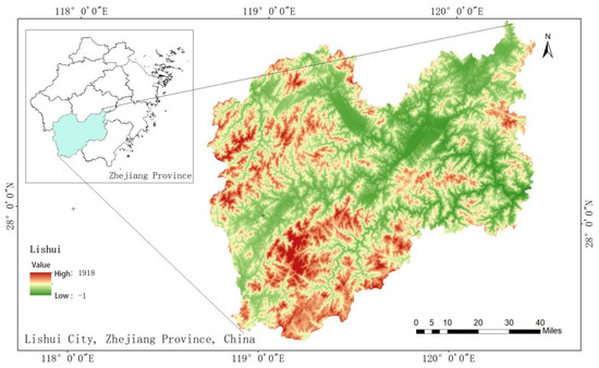
Figure 1.
Map of the study area: Lishui City, Zhejiang Province, China.
2.2. Data
The research data were derived from the 2020 Second National Forest Inventory of Lishui City, Zhejiang Province, focusing on mixed forest sub-compartments dominated by coniferous mixed forest, broadleaved mixed forest, and mixed coniferous–broadleaved forests, totaling 95,730 sub-compartments. Key survey variables for each sub-compartment included elevation, aspect, slope position, slope gradient, soil type, humus layer thickness, average diameter at breast height (DBH), dominant species, age, tree height, and species composition. For constructing the site form model, the growth factors of average DBH and average tree height were utilized. In developing the classification model, site factors such as elevation, aspect, slope position, and slope gradient were selected based on prior research. The growth and site factors for the sample sub-compartments are summarized in Table 1.

Table 1.
Statistical analysis of growth factors and site factors.
This study also requires climate data as independent variables to construct the site classification model. The climate data were sourced from WorldClim (http://www.worldclim.org, accessed on 10 July 2024) [26]. Sixteen climate factors that significantly influence tree growth, including temperature and precipitation, were selected for the analysis. Details of these climate factors are provided in Table 2.
Table 2.
Statistical analysis of climatic factors.
2.3. TWINSPAN Classification Methodology
In forest ecology, commonly used clustering methods include hierarchical clustering, k-means clustering, and the TWINSPAN method. Hierarchical clustering offers intuitive and visually interpretable tree-like structures but becomes computationally intensive when applied to large datasets. K-means clustering is computationally efficient but requires predefining the number of clusters and assumes that clusters have a spherical distribution, which may not align with the complex ecological gradients found in mixed forests. The Two-way Indicator Species Analysis (TWINSPAN) method is a modified form of indicator species analysis and is primarily used as a classification algorithm for simultaneously categorizing sample plots and species [27]. TWINSPAN employs axes derived from Correspondence Analysis (CA) or Detrended Correspondence Analysis (DCA) to progressively refine hierarchical divisions within the dataset, creating an ordered two-way table that categorizes objects (sample plots) and variables (species) [28].
The concept of pseudo-species is introduced in the TWINSPAN classification, which assumes that the same species can have different indicative meanings at varying abundance levels. Thus, these are treated as distinct “species” during analysis. Based on the tree species composition characteristics of mixed forests in Lishui City, Zhejiang Province, tree species abundance was categorized into five levels (0, 2, 4, 6, 8), considering the proportion of species composition comprehensively.
The specific steps of TWINSPAN used in this study are as follows:
First, the sub-compartment data were classified into three major categories—coniferous mixed forest, broadleaved mixed forest, and mixed coniferous–broadleaved forests—based on dominant species. After removing outliers and missing values using a three-standard deviation criterion, 52,876, 9572, and 33,282 records were retained, respectively.
The original data matrix was constructed based on the species composition of the mixed forests, recorded as percentages. These composition percentages formed the basis of the original data matrix (Equation (1)).
The structure of the matrix used in this study is described in Appendix A: where the matrix is a row vector composed of tree species names; the matrix is the stand volume percentage of the corresponding tree species in each sample site consisting of the matrix; m is the number of tree species in the sub-compartments, and n is the number of sub-compartments, i.e., n = 52,876, 9572, 33,282, and m = 39, 36, 41.
The twinspanR package in R (v 4.3.3) was used to perform TWINSPAN analysis. For the coniferous mixed forest, the maximum level of division was set to 3, with pseudo-species cut levels at 0, 2, 4, 6, and 8. For the broadleaved mixed forest and mixed coniferous–broadleaved forests, the maximum level of division was set to 4, using the same pseudo-species cut levels (0, 2, 4, 6, and 8). These parameters were applied to generate the classification results.
2.4. Mixed Forested Site Form Models
2.4.1. Determination of Base Diameter at Breast Height for Mixed Forests
Site form refers to the relationship between dominant height and dominant diameter at breast height (DBH) within a stand, and it requires determining a reference DBH that represents stable height growth while sensitively reflecting site quality differences [29]. Based on the literature and available quantitative methods for calculating reference DBH, this study uses the most frequently occurring DBH value in the research data as the reference DBH [11]. Additionally, since the second national forest inventory does not include data on the average dominant height of trees, and mixed forests are minimally affected by human activities like logging, average tree height is used as a proxy for dominant height.
2.4.2. Guiding Curve Selection
Within the cluster of mean height growth curves for dominant trees in a stand, there is a curve that represents the average growth trajectory of dominant tree height under neutral site conditions as stand age or mean DBH changes. This is known as the guiding curve [30,31]. The choice of guiding curve has a direct impact on the accuracy of site quality assessments. In this study, six commonly used theoretical growth guiding curves—Korf, Schumacher, Richards, Logistic, Compertz, and Weibull—were selected. The expressions for each equation are shown in Table 3.
Table 3.
The theoretical growth models.
2.4.3. Construction of Site Form Models
The algebraic difference approach (ADA) is widely used to model stand growth processes and is one of the most common methods for establishing site index curves [32,33,34,35]. Its principle involves selecting a theoretical equation as the base model and identifying one parameter as the elimination variable. By eliminating this parameter, a difference equation containing two sets of dependent and independent variables is derived. In this study, the optimal guiding curves—Richards, Logistic, Compertz, and Weibull models—were chosen as the base equations for the site form model, with their respective expressions shown in Equations (2)–(5).
where d2 denotes the baseline diameter at breast height (DBH); d1 denotes the dominant diameter at breast height (DBH); H1 denotes the dominant height at DBH d1; parameter a represents the maximum potential growth of trees, parameter c represents the growth rate of trees, and parameter b is used as an elimination parameter to obtain the elimination.
2.5. Machine Learning Algorithms
This study employs two traditional classification algorithms—K-Nearest Neighbors (KNN) and Support Vector Machine (SVM)—along with two ensemble learning algorithms—Random Forest (RF) and XGBoost—to construct site quality classification models. The dataset is divided into a 7:3 ratio for training and testing to ensure robust evaluation and validation of the models.
2.5.1. Random Forest Algorithm
Random Forest (RF) is a classic, straightforward ensemble learning algorithm [36,37] known for its high classification accuracy and ability to handle high-dimensional data [38]. Random Forest uses decision trees as base estimators, training multiple decision trees and combining their outputs to produce a final result [39]. Additionally, RF randomly selects features and samples during training, which helps prevent overfitting and reduces the impact of irrelevant or inconsistent data on the model’s performance [40].
2.5.2. Support Vector Machine Algorithm
Support Vector Machine (SVM) is a supervised learning algorithm that seeks an optimal hyperplane in feature space to separate data points [41]. Before the advent of deep learning, SVM was regarded as one of the most successful and effective machine learning algorithms over the past decade, especially suited for high-dimensional data with low sample sizes. Its core idea is to maximize the margin between two classes of data points, thereby defining a clear decision boundary. Furthermore, with the use of kernel functions [42], SVM can map data into higher-dimensional spaces to address nonlinear problems present in the original features. The advantages of SVM include its ability to handle high-dimensional data, robust performance against noise and outliers, and strong generalization capabilities [43,44,45].
2.5.3. K-Nearest Neighbors Algorithm
The K-Nearest Neighbors (KNN) algorithm is one of the traditional machine learning classification algorithms. It predicts the class of a new data point by measuring its distance from each point in the training set [46]. The core idea of KNN is based on the principle of “similarity”, meaning that similar points are close to each other in feature space. KNN is theoretically well-established and widely used in fields such as data analysis. The algorithm identifies the K closest neighbors to the new data point and assigns its class based on the majority class among these neighbors. KNN is easy to understand theoretically and relatively simple to implement in practice.
2.5.4. XGBoost Algorithm
XGBoost is an efficient machine learning algorithm [47] and an optimized version of Gradient Boosting Decision Trees (GBDTs). It iteratively adds new trees to improve the model while incorporating a regularization term in the loss function to prevent overfitting. XGBoost supports parallel processing, enabling it to leverage multi-core processors to accelerate training, and it can automatically handle missing values, making it highly adaptable [48]. The algorithm performs exceptionally well on large-scale datasets and is widely used for various machine learning tasks, including classification, regression, and ranking [49].
2.6. Model Evaluation and Testing
2.6.1. Indicators for the Evaluation of the Site Form Model
Model simulation and validation are critical steps in the modeling process, focusing on both the significance of the model and its statistical fit. In this study, commonly used regression evaluation metrics, including the coefficient of determination (R2), root mean square error (RMSE), and mean absolute error (MAE), were selected as primary indicators for assessing model performance. Specifically, R2 and RMSE were calculated using fitted sample data, with R2 values closer to 1 and lower RMSE values indicating better model fit. MAE, on the other hand, was evaluated using independent test samples, with smaller MAE values reflecting improved predictive accuracy. To further assess the stability of the guidance curve equations, Akaike Information Criterion (AIC) and Bayesian Information Criterion (BIC) were used as secondary evaluation metrics. AIC and BIC balance model complexity with goodness of fit, where lower values indicate a model that effectively explains the data while avoiding overfitting. Together, these metrics ensure that the selected model achieves both high predictive accuracy and robustness. The formulas for these metrics are as follows:
where R2 is the coefficient of determination; RMSE is the root mean square error; MAE is the mean absolute error; n is the number of samples; , yi, and are the mean average height, the sample measured value of mean height, and the model predicted value of each sample point, respectively; k is the number of estimated parameters in the model; and is the maximum likelihood of the model.
2.6.2. Machine Learning Classification Model Evaluation Metrics
In this study, commonly used evaluation metrics for classifiers, including accuracy, precision, and F1-score, were applied. Accuracy represents the ratio of correctly classified samples to the total number of samples. Precision measures the ratio of correctly predicted positive samples to the total predicted positive samples. F1-score is the harmonic mean of recall and precision, with a value ranging from 0 to 1; values closer to 1 indicate better model performance, while values closer to 0 indicate poorer performance. The expressions for these metrics are shown in Equations (11)–(14).
where TP, TN, FP, and FN are the first letters indicating the results of judgment of real and predicted values, T indicates that the judgment matches, F indicates that the judgment does not match, and the second letter indicates that the classifier predicts the results; P is the judgment of the positive cases and N is the judgment of the negative cases.
3. Results
3.1. TWINSPAN Classification Results
The TWINSPAN classification results for coniferous mixed forests are shown in Figure 2a. After three divisions, the 52,876 coniferous mixed forest sub-compartments were classified into seven groups. Groups D7 and D13 were excluded due to insufficient data. The classification results for broadleaved mixed forest are shown in Figure 2b, where four divisions classified the 9572 sub-compartments into five groups, with Group D3 omitted due to insufficient data. Similarly, the classification results for mixed coniferous–broadleaved forests are shown in Figure 2c. Four divisions classified the 33,282 sub-compartments into five groups, with Group D3 excluded due to insufficient data. After removing misclassified sub-compartments and incorporating sub-compartment composition information, the 15 types of mixed forests and their respective sub-compartment numbers are summarized in Table 4.
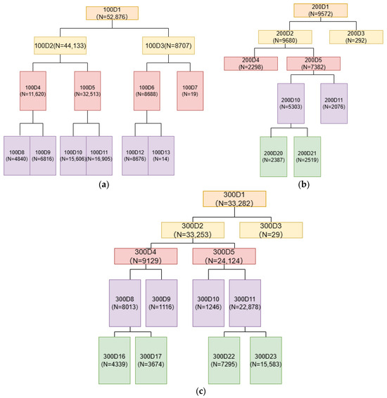
Figure 2.
TWINSPAN classification results of mixed forests: (a) Coniferous mixed forest; (b) broadleaved mixed forest; (c) mixed coniferous–broadleaved forests. Note: ‘D’ is the sample subgroup and ‘N’ is the number of small groups.
Table 4.
Fifteen mixed forest types and number of sub-compartments.
3.2. Fitting Results of the Guidance Curve
The guiding curve fitting was performed using the scientific computing libraries numpy and scipy in Python. Table 5, Table 6 and Table 7 present the fitting results of the foundational height–DBH equations for the 15 groups. The best-fitting results for coniferous mixed forests, broadleaved mixed forests, and mixed coniferous–broadleaved forests are shown in Figure 3.
Table 5.
Coniferous mixed forests guided curve fitting and evaluation.
Table 6.
Broadleaved mixed forests guided curve fitting and evaluation.
Table 7.
Mixed coniferous–broadleaved forests guided curve fitting and evaluation.
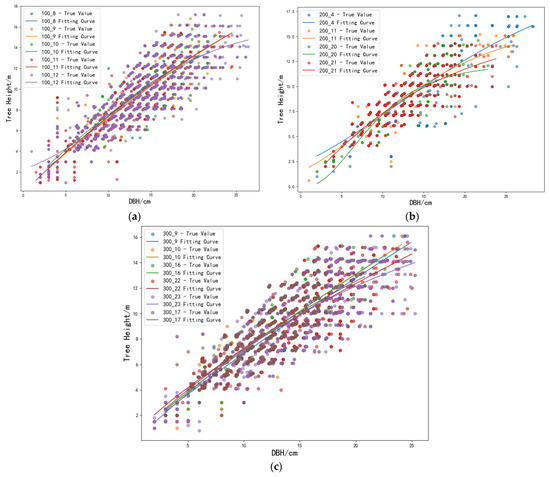
Figure 3.
Best fitting results of the guide curves: (a) Coniferous mixed forest; (b) broadleaved mixed forest; (c) mixed coniferous–broadleaved forests.
Based on the directional curve fitting results for coniferous mixed forests (Table 5), the Compertz equation demonstrated the highest coefficient of determination (R2 = 0.655) for Group 1, with a root mean square error (RMSE) of 1.197 and AIC and BIC values of 1748.251 and 1767.705, respectively. For Group 2, the Weibull equation achieved an R2 of 0.681, an RMSE of 1.251, and AIC and BIC values of 3058.261 and 3078.742, respectively. In Group 3, the Weibull equation showed an R2 of 0.680, an RMSE of 1.052, and a mean absolute error (MAE) of 0.795. For Group 4, the Weibull equation obtained an R2 of 0.757, an RMSE of 1.068, and an MAE of 0.830, with AIC and BIC values of 2226.936 and 2250.143, which were lower than those of the Richards equation. Finally, for Group 5, the Logistic equation achieved an R2 of 0.688, an RMSE of 1.325, and an MAE of 1.055, with AIC and BIC values of 4889.085 and 4910.29. These results indicate that the Compertz equation is the optimal directional curve for Group 1, the Weibull equation is optimal for Groups 2, 3, and 4, and the Logistic equation is the best fit for Group 5.
Based on the directional curve fitting results for broadleaved mixed forests (Table 6), the Richards equation achieved a coefficient of determination (R2) of 0.742 for Group 6, a root mean square error (RMSE) of 1.222, a mean absolute error (MAE) of 0.871, and AIC and BIC values of 893.092 and 910.312, respectively. For Group 7, the Richards equation yielded an R2 of 0.711, an RMSE of 1.032, an MAE of 0.781, an AIC and a BIC values of 138.232 and 155.147. In Group 8, the Compertz equation demonstrated an R2 of 0.767, an RMSE of 0.955, and an MAE of 0.734, which was slightly higher than that of the Richards equation. For Group 9, the Richards, Compertz and Weibull equations had identical R2 (0.723), RMSE (1.022), and MAE (0.797), but the Compertz equation achieved lower AIC and BIC values of 113.510 and 131.005, respectively. These results indicate that the Richards equation is the optimal directional curve for Groups 6 and 7, while the Compertz equation is the best fit for Groups 8 and 9.
Based on the directional curve fitting results for mixed coniferous–broadleaved forests (Table 7), the Richards equation for Group 10 achieved a coefficient of determination (R2) of 0.684, a root mean square error (RMSE) of 1.266, and a mean absolute error (MAE) of 1.035. For Group 11, the Richards equation demonstrated an R2 of 0.822, an RMSE of 1.048, an MAE of 0.822, and AIC and BIC values of 117.572 and 132.956. For Group 12, the Richards equation yielded an R2 of 0.716, an RMSE of 1.117, and an MAE of 0.878. In Group 13, Korf, Richards, and Weibull equations exhibited identical R2 (0.636), RMSE (1.096), and MAE (0.893); however, the Weibull equation had lower AIC and BIC values of 678.024 and 696.652, respectively. For Group 14, the Richards equation achieved an R2 of 0.693, an RMSE of 1.127, an MAE of 0.875, an AIC of 1751.099, and a BIC of 1771.784. In Group 15, the Richards equation attained an R2 of 0.720, an RMSE of 1.067, an MAE of 0.841, an AIC and a BIC values of 2032.566 and 2055.528. These results indicate that the Richards equation is the optimal directional curve for Groups 10, 11, 12, 14, and 15, while the Weibull equation is the best fit for Group 13.
Based on the previous research results, the optimal guiding curve and estimated model parameters for each of the 15 data groups were compiled, as shown in Table 8.
Table 8.
Estimates of the parameters of the optimal guidance curve model and baseline breast diameter.
3.3. Results of the SF Models
Based on the fitting results of the optimal guiding curves, the Richards, Logistic, Weibull, and Compertz equations were selected as the basic equations. Parameter b was eliminated in each case, yielding the model expressions shown in Equations (2)–(5). Using the estimated values of parameters a and c from the optimal guiding curves in Table 8, along with the reference DBH, the site form model expressions for each group were derived, as presented in Table 9.
Table 9.
Site form model expressions.
3.4. Site Grade Division
Using the formulas in Table 9, the site form (SF) for each sub-compartment within each group was calculated and classified into three levels: high, medium, and low. Efforts were made to ensure a balanced sample size across categories. To objectively validate the classification and grouping rationale, an analysis of variance (ANOVA) was conducted to examine differences in tree height, diameter at breast height (DBH), and stand volume among the three levels. The results demonstrated statistically significant differences among the three levels (p < 0.05), confirming that classifying site quality into three levels—Grade I (high-quality sites), Grade II (medium-quality sites), and Grade III (low-quality sites)—is reasonable and effective. The distribution of SF values and the number of sub-compartments within each group are summarized in Table 10.
Table 10.
Frequency distribution of SF in sub-compartments of mixed forests.
3.5. Comparison of Classification Results of Machine Learning Algorithms
3.5.1. Data Processing
According to the data analysis, the distribution of data across different site categories is imbalanced, which can negatively affect the accuracy of the final classification model. To address this imbalance and achieve a more balanced sample distribution, the Synthetic Minority Over-sampling Technique (SMOTE) was applied. SMOTE is a widely used oversampling method for handling imbalanced data in classification tasks. The principle of SMOTE is to generate new samples by randomly creating a point between two minority class samples based on their distance, ensuring that the new sample lies between the two original minority class samples.
Considering the significant multicollinearity among environmental variables, which may lead to overfitting or reduced predictive performance, rigorous variable selection was performed prior to model construction. Variance Inflation Factor (VIF) was employed as the evaluation metric to assess the multicollinearity among variables. VIF quantifies the degree of linear correlation between a variable and other variables. A VIF value exceeding 10 indicates substantial multicollinearity, which could adversely affect the model’s stability and interpretability. Following this criterion, we conducted iterative screening of the initial variable set, removing variables with VIF > 10 in each round until all remaining variables had VIF values below 10. After multiple iterations, 15 key features were retained as input factors for the model: elevation (VIF = 2.35), slope aspect (VIF = 1.13), slope position (VIF = 1.07), slope gradient (VIF = 2.75), soil type (VIF = 1.01), soil texture (VIF = 1.31), soil thickness (VIF = 1.21), humus layer thickness (VIF = 1.17), understory vegetation height (1.39), monthly average temperature difference (VIF = 8.80), minimum temperature in the coldest month (VIF = 4.43), annual mean temperature range (VIF = 6.55), average temperature in the wettest season (VIF = 2.55), precipitation in the driest month (VIF = 4.48), and precipitation in the wettest quarter (6.14).
3.5.2. Classification Results and Analyses
All Classifier models were constructed on the training set, with primary parameter ranges determined through grid search. Multiple rounds of adjustments were then performed, and the models were evaluated using a validation set. In terms of model assessment, emphasis was placed on overall comprehensive evaluation metrics, as well as class-specific accuracy and F1-score.
The performance metrics in Table 11 clearly demonstrate that the XGBoost model consistently outperforms other models across all groups. In Group 1, XGBoost achieves the highest Precision and F1-score of 0.95, with classification accuracies of 0.98, 0.93, and 0.92 for “Grade I”, “Grade II”, and “Grade III”, respectively. Similarly, in Group 2, XGBoost leads with a Precision and F1-score of 0.92, achieving classification accuracies of 0.99 for “Grade I”, 0.88 for “Grade II”, and 0.89 for “Grade III”. In Group 3, XGBoost continues to perform strongly, with a Precision and F1-score of 0.90 and classification accuracies of 0.89, 0.87, and 0.94 for “Grade I”, “Grade II”, and “Grade III”, respectively. In Group 4, both XGBoost and RF demonstrate superior performance, achieving equal Precision and F1-scores of 0.94. Finally, in Group 5, XGBoost achieves its best performance, with a Precision and F1-score of 0.96 and classification accuracies of 0.98, 0.94, and 0.96 for “Grade I”, “Grade II”, and “Grade III”, respectively. These results conclusively show that XGBoost consistently achieves the highest Precision, F1-score, and classification accuracies, making it the most reliable and effective model for this classification task.
Table 11.
Coniferous mixed forests classification model performance (validation set).
The performance metrics in Table 12 for Groups 6 to 9 demonstrate the consistent superiority of the XGBoost model in most groups. In Group 6, both the XGBoost and RF models have a Precision and F1-score of 0.94, but the accuracy for “Grade I” and “Grade II” is higher than that of the RF model, with values of 0.93 and 0.93, respectively. Similarly, in Group 7, XGBoost leads with a Precision and F1-score of 0.89, achieving classification accuracies of 0.83, 0.86, and 0.98 for “Grade I”, “Grade II”, and “Grade III”, respectively. In Group 8, the RF model performs best, with a Precision and F1-score of 0.93, slightly surpassing XGBoost’s 0.92. Finally, in Group 9, XGBoost matches RF with a Precision of 0.91 but surpasses all other models in classification accuracies for “Grade II” (0.90) and “Grade III” (0.88). Overall, XGBoost demonstrates superior and stable performance across most groups, establishing itself as the most effective model for this classification task.
Table 12.
Classification model performance for broadleaved mixed forests (validation set).
The performance metrics for Groups 10 to 15 in Table 13 indicate that the XGBoost model excels in most groups. In Group 10, the RF model outperforms XGBoost with a Precision and F1-score of 0.81 and 0.80, respectively. In Group 11, both RF and SVM show the best performance, with Precision and F1-scores of 0.93. In Group 12, both XGBoost and SVM achieve Precision and F1-scores of 0.84, but XGBoost outperforms SVM in “Grade I” and “Grade III”. In Group 13, XGBoost and RF have similar performance, with close Precision and F1-scores. In Group 14, XGBoost achieves the best performance, with Precision and F1-scores of 0.97 and classification accuracies for “Grade I”, “Grade II”, and “Grade III” of 0.96, 0.96, and 0.99, respectively. Finally, in Group 15, XGBoost performs best, with a Precision and F1-score of 0.96 and classification accuracies for “Grade I”, “Grade II”, and “Grade III” of 0.98, 0.94, and 0.96, respectively.
Table 13.
Mixed coniferous–broadleaved forests classification model performance (validation set).
To provide a clearer understanding and assessment of site quality types for mixed forests in the study area, ArcGIS (v10.8) was utilized to generate a visual classification map for the three mixed forest types in Lishui, Zhejiang Province. As depicted in Figure 4, the site quality of mixed forests in Lishui is predominantly classified as Grade II, with Grades I and III being relatively less frequent. This suggests that the overall site quality in the region is moderate, with a balanced distribution of higher and lower-quality areas. The classification map enables straightforward identification of site quality levels for any mixed forest sub-compartment within Lishui, offering a practical tool for forest reserve zoning, selecting appropriate silvicultural practices, and informing management decisions based on the principle of “suitable species for suitable sites”. Furthermore, the map serves as a valuable reference for biodiversity conservation, as high-quality sites are likely to host diverse species due to their superior environmental conditions. By prioritizing conservation efforts in these areas and adopting targeted interventions in medium and lower-quality sites, the classification supports sustainable forest management and enhances ecological resilience across the region.
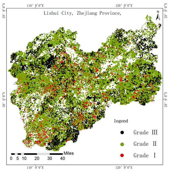
Figure 4.
The predicted site quality classification map of mixed forests.
4. Discussion
This study utilized the TWINSPAN classification method based on forest stand species composition. Sun et al. [50] applied TWINSPAN to analyze the composition of Sassafras communities in Zhejiang Province, classifying 96 sample plots into eight types, each with unique species compositions and environmental characteristics. Similarly, Rahman et al. [51] used TWINSPAN to quantify and classify vegetation into five community types in the Sultan Khel Valley of the Hindu Kush Mountains. Novák et al. [52] applied TWINSPAN hierarchical clustering to a dataset of 15,817 vegetation plots, identifying clusters with similar species composition and ecological–geographical characteristics. In this study, TWINSPAN effectively distinguished 15 types of mixed forests, which were then classified by site quality. Differentiating site quality among various stand types enables a more precise assessment of growth performance under different site conditions, providing insights into each stand type’s adaptability and productivity potential across varying environmental conditions. This approach is crucial for forest planning and resource allocation.
For constructing the site form model, site form represents the relationship between dominant height and DBH, requiring a reference DBH that reflects stable height growth and sensitively captures differences in site quality. The choice of reference DBH significantly impacts the site form model. This study adopted a method that uses the most frequently occurring diameter at breast height (DBH) value within this study’s dataset as the reference DBH. The commonly occurring DBH value accurately represents the growth status of the majority of trees, enhancing the model’s representativeness and applicability. Nevertheless, this method has certain limitations. Using the most frequently observed DBH may overlook the variability within DBH distributions, particularly in cases where the DBH distribution is highly dispersed or multimodal. In such instances, the mode may not accurately reflect the overall growth characteristics of the stand. Additionally, in stands with abnormal DBH distributions or those influenced by external factors, relying on the most frequently observed DBH could underestimate the stand’s productive potential. Apart from the method used in this study, other approaches for selecting reference DBH have been proposed in previous research. These include using half the average DBH typically achieved in the growth history of dominant trees, identifying the DBH at the inflection point of the height–DBH curve (where the second derivative equals zero, indicating a change in growth trend), or deriving the DBH corresponding to a reference age from a DBH–age model. In mixed forests, determining stand age is challenging, while DBH data are readily available, making the application of site form in mixed forest site quality assessment feasible. Identifying the most suitable reference DBH to represent the growth patterns of mixed forest stands remains an important direction for future research. Additionally, obtaining dominant height is essential for site form model calculations. In this study, mean height was used as a substitute for dominant height. However, the diversity of species, natural thinning, and human activities in mixed forests can affect mean height, potentially underestimating site productivity. The use of mean height instead of dominant height is a limitation, and further data collection on dominant height would enhance model accuracy.
In forestry, machine learning algorithms have increasingly become powerful tools for handling high-dimensional, complex nonlinear data [53,54]. Our results indicate that the XGBoost model is an effective method for site quality classification. Using site and climate factors as features, we constructed site quality classification models with two traditional classification algorithms and two ensemble learning algorithms, comparing their performance. All four models achieved overall accuracies above 0.77, with XGBoost consistently performing well across most groups. As a tree-based ensemble learning method, XGBoost improves the accuracy of weak classifiers through weighted boosting and excels on large datasets [55]. While XGBoost demonstrates strong predictive performance, its ecological applications require careful consideration of model complexity and practical requirements. XGBoost has been successfully applied in various forestry tasks, demonstrating its robustness and versatility. For instance, it has been used in tree species identification with hyperspectral data, achieving significantly higher accuracy compared to traditional methods [56]. In forest fire prediction, XGBoost integrated climatic and environmental data to accurately identify high-risk areas, outperforming conventional statistical models [57]. Similarly, in carbon storage estimation, XGBoost effectively modeled the complex relationships between site quality, species composition, and climatic conditions, providing precise predictions for sustainable forest management [58]. These examples illustrate its potential for addressing diverse and complex challenges in forestry.
Despite its powerful predictive capabilities, XGBoost presents some drawbacks in practical applications, particularly its sensitivity to hyperparameters and potential overfitting issues. The model requires careful tuning of hyperparameters, such as learning rate, tree depth, and the proportion of sample subsets. Improper selection of these parameters can lead to model instability or overfitting. In certain situations, especially with small datasets or complex features, XGBoost may overfit, meaning the model performs well on training data but poorly on unseen data, limiting its generalization ability in real-world applications. Nevertheless, machine learning methods like XGBoost can offer valuable tools for site quality assessment, particularly in areas lacking vegetation cover. By integrating site and climatic factors, these models can predict the potential site quality of non-forested areas with high accuracy. Such predictions provide a scientific foundation for tree species selection and afforestation planning, making them especially significant for future forest development and ecological restoration. This approach enables a more targeted and effective restoration process, aligning with sustainable forestry practices and improving the ecological resilience of mixed forests. While the model proposed here is specific to Lishui City, Zhejiang Province, it has broad potential for application in other regions and non-forested areas. In the future, classification models can be developed for different regions with varying environmental conditions and forest types, further enhancing the versatility and applicability of the method. This adaptability makes the approach valuable for large-scale ecological restoration and sustainable land management practices.
5. Conclusions
Due to the complex species composition and age structure of mixed forests, the evaluation of site quality in these forests remains an ongoing area of exploration. To address the challenges in mixed forest site quality assessment, this study focuses on the mixed forests of Lishui City, Zhejiang Province. First, the TWINSPAN method was applied to classify the mixed forests into 15 stand types. Then, the Algebraic Difference Approach (ADA) was used to develop a site form model, which enabled the classification of site quality levels for each of the 15 stand types. Based on these classifications and incorporating site and climate factors, a site quality classification model for mixed forests was constructed using multiple machine learning algorithms. Finally, a comparative analysis was conducted to identify the most suitable classification model. This study provides a comprehensive workflow for data processing, modeling, and evaluation and uses the optimal model to classify and visually display site quality levels for mixed forest sub-compartments in the study area.
Comparison of model performance before and after applying SMOTE, see Supplementary Materials.
Supplementary Materials
The following supporting information can be downloaded at: https://www.mdpi.com/article/10.3390/f15122247/s1.
Author Contributions
Conceptualization, R.W. and W.G.; Methodology, R.W., C.D. and W.G.; Investigation, R.W. and C.Z.; Writing—original draft, R.W. and C.D.; Project administration, R.W.; Data curation, C.D.; Funding acquisition, C.D.; Resources, C.D. and C.Z.; Supervision, X.L.; Writing—review and editing, X.Z. All authors have read and agreed to the published version of the manuscript.
Funding
This research was funded by the National Natural Science Foundation of China (32301585).
Data Availability Statement
The data are available on request from the corresponding author.
Acknowledgments
We are grateful to the Zhejiang Forest Resources Monitoring Center for supplying the valuable model data. We would also like to express our gratitude to the English language editors, who helped with checking grammatical mistakes.
Conflicts of Interest
The authors declare no conflicts of interest.
Appendix A
The structure of the matrix used in this study is described as follows:
- Matrix Definition:
- o
- : A row vector composed of the names of all tree species that appear across the sub-compartments, where m represents the total number of tree species.
- o
- : An matrix composed of the stand volume percentages of the corresponding tree species in each sub-compartment, where n represents the total number of sub-compartments.
- Parameter Description:
- o
- m: The total number of tree species appearing in all sub-compartments.
- o
- n: The total number of sub-compartments.
- Specific Cases:
- o
- Coniferous Mixed Forests: A total of m = 39 tree species and n = 52,876 sub-compartments.
- o
- Broadleaved Mixed Forest: A total of m = 36 tree species and n = 9572 sub-compartments.
- o
- Mixed coniferous–broadleaved forests: A total of m = 41 tree species and n = 33,282 sub-compartments.
References
- Meng, X.Y. Forest Measurements; China Forestry Publishing House: Beijing, China, 2006. [Google Scholar]
- Everett, C.J.; Thorp, J.H. Site Quality Evaluation of Loblolly Pine on the South Carolina Lower Coastal Plain, USA. J. For. Res. 2008, 19, 187–192. [Google Scholar] [CrossRef]
- Louw, J.H.; Scholes, M. Forest Site Classification and Evaluation: A South African Perspective. For. Ecol. Manag. 2002, 171, 153–168. [Google Scholar] [CrossRef]
- Min, Z.; Wu, B.; Su, X.; Chen, Y.; Tian, Y. Suitability Evaluation and Dominant Function Model for Multifunctional Forest Management. Forests 2020, 11, 1368. [Google Scholar] [CrossRef]
- Batho, A.; Garcia, O. De Perthuis and the Origins of Site Index: A Historical Note. FBMIS 2006, 1, 1–10. [Google Scholar]
- Noordermeer, L.; Bollandsås, O.M.; Gobakken, T.; Næsset, E. Direct and Indirect Site Index Determination for Norway Spruce and Scots Pine Using Bitemporal Airborne Laser Scanner Data. For. Ecol. Manag. 2018, 428, 104–114. [Google Scholar] [CrossRef]
- Yan, X.; Feng, L.; Sharma, R.P.; Duan, G.; Pang, L.; Fu, L.; Guo, J. Evaluating Forest Site Quality Using the Biomass Potential Productivity Approach. Forests 2023, 15, 23. [Google Scholar] [CrossRef]
- Berrill, J.-P.; O’Hara, K.L. Estimating Site Productivity in Irregular Stand Structures by Indexing the Basal Area or Volume Increment of the Dominant Species. Can. J. For. Res. 2014, 44, 92–100. [Google Scholar] [CrossRef]
- Luo, Y.; Yang, Y.-C.; Wang, J.; Ji, L.; Liu, T.; Yu, H.-Y.; LI, Y.; Wang, Y.-X. Site Index Model of Juglans Mandshurica Natural Secondary Mixed Forest in Changbai Mountain Area, Jilin Province, China. Chin. J. Appl. Ecol. 2019, 30, 4049–4058. [Google Scholar] [CrossRef]
- Ercanli, İ.; KahriMan, A.; Yavuz, H. Dynamic Base-Age Invariant Site Index Models Based on Generalized Algebraic Difference Approach for Mixed Scots Pine (Pinus sylvestris L.) and Oriental Beech (Fagus orientalis Lipsky) Stands. Turk. J. Agric. For. 2014, 38, 134–147. [Google Scholar] [CrossRef]
- Vanclay, J.K.; Henry, N.B. Assessing Site Productivity of Indigenous Cypress Pine Forest in Southern Queensland. Commonw. For. Rev. 1988, 67, 53–64. [Google Scholar]
- Gao, W.; Dong, C.; Gong, Y.; Ma, S.; Shen, J.; Lin, S. Site Quality Evaluation Model of Chinese Fir Plantations for Machine Learning and Site Factors. Sustainability 2023, 15, 15587. [Google Scholar] [CrossRef]
- Herrera-Fernández, B.; Campos, J.J.; Kleinn, C. Site Productivity Estimation Using Height-Diameter Relationships in Costa Rican Secondary Forests. For. Syst. 2004, 13, 295–303. [Google Scholar] [CrossRef]
- Do, H.T.T.; Zimmer, H.C.; Vanclay, J.K.; Grant, J.C.; Trinh, B.N.; Nguyen, H.H.; Nichols, J.D. Site Form Classification—A Practical Tool for Guiding Site-Specific Tropical Forest Landscape Restoration and Management. For. Int. J. For. Res. 2022, 95, 261–273. [Google Scholar] [CrossRef]
- Castaño-Santamaría, J.; López-Sánchez, C.A.; Obeso, J.R.; Barrio-Anta, M. Development of a Site Form Equation for Predicting and Mapping Site Quality. A Case Study of Unmanaged Beech Forests in the Cantabrian Range (NW Spain). For. Ecol. Manag. 2023, 529, 120711. [Google Scholar] [CrossRef]
- Barnes, B. The Ecological Approach to Ecosystem Classification. In Proceedings of the IUFRO Symposium on Site and Productivity of Fast Growing Plantations, Pretoria and Pietermaritzburg, South Africa, 30 April–11 May 1984; Volume 30, pp. 69–89. [Google Scholar]
- Tesch, S.D. The Evolution of Forest Yield Determination and Site Classification. For. Ecol. Manag. 1980, 3, 169–182. [Google Scholar] [CrossRef]
- Zhang, P.; Lu, W.; Xu, J.; Lin, Z.; Chen, M.; Li, K. Site Classification and Quality Evaluation of Eucalyptus urophylla × E. tereticornis Plantation in Hainan Island and Leizhou Peninsula Region. For. Sci. Res. 2021, 34, 130–139. [Google Scholar] [CrossRef]
- Lu, H.; Xu, J.; Li, G.; Liu, W. Site Classification of Eucalyptus urophylla × Eucalyptus grandis Plantations in China. Forests 2020, 11, 871. [Google Scholar] [CrossRef]
- Zhang, X.; Yu, Q.; Luo, G.; Jia, X.; Wu, D.; Jia, Z. Site Classification and Site Quality Evaluation of Pinus Tabulaeformis Plantation for Construction Timber in Pingquan, Hebei Province. Master’s Thesis, Beijing Forestry University, Beijing, China, 2021. [Google Scholar]
- Liu, Z.; Peng, C.; Work, T.; Candau, J.-N.; DesRochers, A.; Kneeshaw, D. Application of Machine-Learning Methods in Forest Ecology: Recent Progress and Future Challenges. Environ. Rev. 2018, 26, 339–350. [Google Scholar] [CrossRef]
- Zhao, Q.; Yu, S.; Zhao, F.; Tian, L.; Zhao, Z. Comparison of Machine Learning Algorithms for Forest Parameter Estimations and Application for Forest Quality Assessments. For. Ecol. Manag. 2019, 434, 224–234. [Google Scholar] [CrossRef]
- Pereira Martins Silva, J.; Luiza Marques da Silva, M.; Ribeiro de Mendonça, A.; Fernandes da Silva, G.; Almeida de Barros Junior, A.; Ferreira da Silva, E.; Otone Aguiar, M.; Silva Santos, J.; Maria Mafra Rodrigues, N. Prognosis of Forest Production Using Machine Learning Techniques. Inf. Process. Agric. 2023, 10, 71–84. [Google Scholar] [CrossRef]
- Piri Sahragard, H.; Ajorlo, M.; Karami, P. Modeling Habitat Suitability of Range Plant Species Using Random Forest Method in Arid Mountainous Rangelands. J. Mt. Sci. 2018, 15, 2159–2171. [Google Scholar] [CrossRef]
- Chen, Y.; Wu, B.; Chen, D.; Qi, Y. Using Machine Learning to Assess Site Suitability for Afforestation with Particular Species. Forests 2019, 10, 739. [Google Scholar] [CrossRef]
- Hijmans, R.J.; Cameron, S.E.; Parra, J.L.; Jones, P.G.; Jarvis, A. Very High Resolution Interpolated Climate Surfaces for Global Land Areas. Int. J. Climatol. 2005, 25, 1965–1978. [Google Scholar] [CrossRef]
- Zhang, H. Classification and Succession Analysis of Mixed Forest in Jingouling Forest Farm Using the TWINSPAN Method. J. Nanjing For. Univ. 2009, 33, 37–42. [Google Scholar]
- Hill, M.O. A FORTRAN Program for Arranging Multivariate Data in an Ordered Two-Way Table by Classification of the Individuals and Attributes. In Section of Ecology and Systematica; Cornell University: Ithaca, NY, USA, 1979. [Google Scholar]
- Vanclay, J.K. Modelling Forest Growth and Yield: Applications to Mixed Tropical Forests; CAB International: Wallingford, UK, 1994. [Google Scholar]
- Marchand, W.; Buechling, A.; Rydval, M.; Čada, V.; Stegehuis, A.I.; Fruleux, A.; Poláček, M.; Hofmeister, J.; Pavlin, J.; Ralhan, D.; et al. Accelerated Growth Rates of Norway Spruce and European Beech Saplings from Europe’s Temperate Primary Forests Are Related to Warmer Conditions. Agric. For. Meteorol. 2023, 329, 109280. [Google Scholar] [CrossRef]
- Zhang, Y.; Dong, L.; Xie, Y.; Chen, D.; Sun, X. Altitude Shape Genetic and Phenotypic Variations in Growth Curve Parameters of Larix Kaempferi. J. For. Res. 2023, 34, 507–517. [Google Scholar] [CrossRef]
- Clutter, J.L. Compatible Growth and Yield Models for Loblolly Pine. For. Sci. 1963, 9, 354–371. [Google Scholar]
- Bailey, R.L.; Clutter, J.L. Base-Age Invariant Polymorphic Site Curves. For. Sci. 1974, 20, 155–159. [Google Scholar]
- Anta, M.B.; Dorado, F.C.; Diéguez-Aranda, U.; Álvarez González, J.G.; Parresol, B.R.; Soalleiro, R.R. Development of a Basal Area Growth System for Maritime Pine in Northwestern Spain Using the Generalized Algebraic Difference Approach. Can. J. For. Res. 2006, 36, 1461–1474. [Google Scholar] [CrossRef]
- Zobel, J.M.; Schubert, M.R.; Granger, J.J. Shortleaf Pine (Pinus echinata) Site Index Equation for the Cumberland Plateau, USA. For. Sci. 2022, 68, 259–269. [Google Scholar] [CrossRef]
- Breiman, L. Random Forests. Mach. Learn. 2001, 45, 5–32. [Google Scholar] [CrossRef]
- Dong, C.; Chen, Y.; Lou, X.; Min, Z.; Bao, J. Site Quality Classification Models of Cunninghamia lanceolata Plantations Using Rough Set and Random Forest West of Zhejiang Province, China. Forests 2022, 13, 1312. [Google Scholar] [CrossRef]
- Ye, Y.; Wu, Q.; Zhexue Huang, J.; Ng, M.K.; Li, X. Stratified Sampling for Feature Subspace Selection in Random Forests for High Dimensional Data. Pattern Recognit. 2013, 46, 769–787. [Google Scholar] [CrossRef]
- Sun, Z.; Wang, G.; Li, P.; Wang, H.; Zhang, M.; Liang, X. An Improved Random Forest Based on the Classification Accuracy and Correlation Measurement of Decision Trees. Expert Syst. Appl. 2024, 237, 121549. [Google Scholar] [CrossRef]
- Louppe, G. Understanding Random Forests: From Theory to Practice. arXiv 2014, arXiv:1407.7502. [Google Scholar]
- Cortes, C.; Vapnik, V. Support-Vector Networks. Mach. Learn. 1995, 20, 273–297. [Google Scholar] [CrossRef]
- Burges, C.J.C. A Tutorial on Support Vector Machines for Pattern Recognition. Data Min. Knowl. Discov. 1998, 2, 121–167. [Google Scholar] [CrossRef]
- Cervantes, J.; Garcia-Lamont, F.; Rodríguez-Mazahua, L.; Lopez, A. A Comprehensive Survey on Support Vector Machine Classification: Applications, Challenges and Trends. Neurocomputing 2020, 408, 189–215. [Google Scholar] [CrossRef]
- Xu, L. Robust Support Vector Machine Training via Convex Outlier Ablation. In Proceedings of the Twenty-First National Conference on Artificial Intelligence and the Eighteenth Innovative Applications of Artificial Intelligence Conference, Boston, MA, USA, 16–20 July 2006. [Google Scholar]
- Cover, T.M.; Hart, P.E. Nearest Neighbor Pattern Classification. IEEE Trans. Inf. Theory 1967, 13, 21–27. [Google Scholar] [CrossRef]
- Zhang, S.; Li, X.; Zong, M.; Zhu, X.; Cheng, D. Learning k for kNN Classification. ACM Trans. Intell. Syst. Technol. 2017, 8, 1–19. [Google Scholar] [CrossRef]
- Reddy, S.; Akashdeep, S.; Harshvardhan, R.; Kamath, S. Stacking Deep Learning and Machine Learning Models for Short-Term Energy Consumption Forecasting. Adv. Eng. Inform. 2022, 52, 101542. [Google Scholar] [CrossRef]
- Wang, M.; Fu, W.; He, X.; Hao, S.; Wu, X. A Survey on Large-Scale Machine Learning. IEEE Trans. Knowl. Data Eng. 2022, 34, 2574–2594. [Google Scholar] [CrossRef]
- Chen, T.; Guestrin, C. XGBoost: A Scalable Tree Boosting System. In Proceedings of the 22nd ACM SIGKDD International Conference on Knowledge Discovery and Data Mining, San Francisco, CA, USA, 13 August 2016; ACM: New York, NY, USA; pp. 785–794. [Google Scholar]
- Sun, J.; Guo, J.; Shen, A.; Xu, X.; Feng, H.; Zhang, S.; Yuan, W.; Jiang, B.; Wu, C.; Wang, W. Composition and Environmental Interpretation of the Communities of Sassafras Tzumu, a Protected Species, at Zhejiang Province in Eastern China. Glob. Ecol. Conserv. 2020, 24, e01218. [Google Scholar] [CrossRef]
- Rahman, K.; Akhtar, N. Ecological Evaluation of Vegetation Pattern of Sultan Khail Valley, Hindu Kush Range of Pakistan Using Advance Multivariate Analysis. TechRxiv 2024. [Google Scholar] [CrossRef]
- Novák, P.; Willner, W.; Biurrun, I.; Gholizadeh, H.; Heinken, T.; Jandt, U.; Kollár, J.; Kozhevnikova, M.; Naqinezhad, A.; Onyshchenko, V.; et al. Classification of European Oak–Hornbeam Forests and Related Vegetation Types. Appl. Veg. Sci. 2023, 26, e12712. [Google Scholar] [CrossRef]
- Fang, N.; Yao, L.; Wu, D.; Zheng, X.; Luo, S. Assessment of Forest Ecological Function Levels Based on Multi-Source Data and Machine Learning. Forests 2023, 14, 1630. [Google Scholar] [CrossRef]
- Sheykhmousa, M.; Mahdianpari, M.; Ghanbari, H.; Mohammadimanesh, F.; Ghamisi, P.; Homayouni, S. Support Vector Machine Versus Random Forest for Remote Sensing Image Classification: A Meta-Analysis and Systematic Review. IEEE J. Sel. Top. Appl. Earth Obs. Remote Sens. 2020, 13, 6308–6325. [Google Scholar] [CrossRef]
- Jafarzadeh, H.; Mahdianpari, M.; Gill, E.; Mohammadimanesh, F.; Homayouni, S. Bagging and Boosting Ensemble Classifiers for Classification of Multispectral, Hyperspectral and PolSAR Data: A Comparative Evaluation. Remote Sens. 2021, 13, 4405. [Google Scholar] [CrossRef]
- Zhou, G.; Ni, Z.; Zhao, Y.; Luan, J. Identification of Bamboo Species Based on Extreme Gradient Boosting (XGBoost) Using Zhuhai-1 Orbita Hyperspectral Remote Sensing Imagery. Sensors 2022, 22, 5434. [Google Scholar] [CrossRef]
- Yan, W.; Ren, J.; Feng, J.; Duan, Y.; Wei, C. A New Forest Fire Risk Rating Forecast Model Based on Xgboost. In Proceedings of the 2022 International Seminar on Computer Science and Engineering Technology (SCSET), Indianapolis, IN, USA, 19–21 December 2022; IEEE: New York, NY, USA; pp. 227–230. [Google Scholar]
- Li, Y.; Li, M.; Wang, Y. Forest Aboveground Biomass Estimation and Response to Climate Change Based on Remote Sensing Data. Sustainability 2022, 14, 14222. [Google Scholar] [CrossRef]
Disclaimer/Publisher’s Note: The statements, opinions and data contained in all publications are solely those of the individual author(s) and contributor(s) and not of MDPI and/or the editor(s). MDPI and/or the editor(s) disclaim responsibility for any injury to people or property resulting from any ideas, methods, instructions or products referred to in the content. |
© 2024 by the authors. Licensee MDPI, Basel, Switzerland. This article is an open access article distributed under the terms and conditions of the Creative Commons Attribution (CC BY) license (https://creativecommons.org/licenses/by/4.0/).