PosE-Enhanced Point Transformer with Local Surface Features (LSF) for Wood–Leaf Separation

Abstract

Wood–leaf separation from forest LiDAR point clouds is a challenging task due to the complex and irregular structures of tree canopies. Traditional machine vision and deep learning methods often struggle to accurately distinguish between fine branches and leaves. This challenge arises primarily from the lack of suitable features and the limitations of existing position encodings in capturing the unique and intricate characteristics of forest point clouds. In this work, we propose an innovative approach that integrates Local Surface Features (LSF) and a Position Encoding (PosE) module within the Point Transformer (PT) network to address these challenges. We began by preprocessing point clouds and applying a machine vision technique, supplemented by manual correction, to create wood–leaf-separated datasets of forest point clouds for training. Next, we introduced Point Feature Histogram (PFH) to construct LSF for each point network input, while utilizing Fast PFH (FPFH) to enhance computational efficiency. Subsequently, we designed a PosE module within PT, leveraging trigonometric dimensionality expansion and Random Fourier Feature-based Transformation (RFFT) for nuanced feature analysis. This design significantly enhances the representational richness and precision of forest point clouds. Afterward, the segmented branch point cloud was used to model tree skeletons automatically, while the leaves were incorporated to complete the digital twin. Our enhanced network, tested on three different types of forests, achieved up to 96.23% in accuracy and 91.51% in mean intersection over union (mIoU) in wood–leaf separation, outperforming the original PT by approximately 5%. This study not only expands the limits of forest point cloud research but also demonstrates significant improvements in the reconstruction results, particularly in capturing the intricate structures of twigs, which paves the way for more accurate forest resource surveys and advanced digital twin construction.

1. Introduction

Forest digital twins have revolutionized silvicultural management, ecological landscape design, and land resource investigation by integrating cross-technology communication and offering immersive simulations beyond the constraints of traditional field-based studies [1,2]. They empower users to conduct thinning experiments under diverse climatic scenarios, providing a forward-looking perspective on forest development and ecological dynamics [3]. While not exact replicas, forest digital twins are meticulously designed to support practical forestry applications such as inventorying and predictive forest modeling. By capturing essential behaviors like forest degradation, biodiversity dynamics, and forest–climate–soil interactions, they provide valuable insights for estimating biomass, analyzing canopy structure, and simulating long-term forest evolution [4].

Tree reconstruction methods, as the visual and structural foundation of forest digital twins, have evolved into three main approaches: image-based reconstruction [5,6], point-cloud-based reconstruction [7] and virtual-reality-based modelling [8]. These methods translate raw data into realistic and functional models that enable detailed simulations and analyses. Among these, with the rise of deep learning, some studies have utilized AI to reconstruct realistic trees. TreePartNet [9] reconstructs tree geometry by detecting semantic branching points and learning cylindrical representations of branches, followed by merging these representations into a final set of generalized cylinders to model the tree structure. A framework combining Unet++ for branch segmentation, Point2Skeleton for reconstruction, and a novel Obscured Branch Recovery (OBR) algorithm [10] reconstructs 3D obscured branches from RGBD images for efficient fruit harvesting. Despite differing logic and algorithms, these methods share a common technical focus: wood–leaf segmentation from point clouds.

In the context of point cloud data (PCD) analysis, wood–leaf segmentation is a critical task. Wood–leaf segmentation methods can be broadly classified into two approaches: conventional machine vision and deep-learning-based methods. Conventional machine vision techniques rely on image processing and geometry-based algorithms to analyze and interpret data derived from the natural environment. Leveraging common geometric features (curvature, density, etc.), growing patterns, and topological information [11,12], conventional machine vision techniques facilitate both wood–leaf separation and structural continuity analysis of arboreal elements [13]. Moreover, identifying non-photosynthetic constituents based on segment linearity, along with other methods, enhances the analysis, further augmenting the overall analytical process [14]. Clustering methods such as K-Means [15], LDA [16], and DBSCAN [12,17] serve as valuable auxiliary tools, enhancing the effectiveness of wood–leaf separation in point cloud data and supporting the analysis of structural continuity within tree components. However, these approaches often falter when addressing the challenges posed by occlusions and complex canopy structures, particularly in dense forests. Hao et al. [18] introduced Chaos Distance as a clustering parameter, which exploits the observation that wood points are more orderly while leaf points are more chaotic, providing an improved mechanism for separation under such challenging conditions. Moreover, these methods struggle with efficiently processing large-scale datasets, further hindering their ability to perform accurate wood–leaf segmentation in complex forest environments.

Deep learning techniques, diverging fundamentally from machine vision strategies, underscore their capabilities by exploiting data-driven analysis without needing to comprehend clear-cut physical principles. For instance, MIX-Net [19] employs a linear mixer mechanism to both segment and complete point clouds, but its reliance on a linear structure limits its ability to handle highly complex and non-linear relationships present in natural scenes. Additionally, the convolution operation faces challenges when applied to non-rigid tree PCDs with irregular and sparse points, which lack logical relations and permutation invariance, further hindering effective segmentation. Alternatively, PSegNet [20] simplifies samples during semantic segmentation of plant structures by employing a double-neighborhood feature extraction block (DNFEB) and a double-granularity feature fusion module (DGFFM), but it faces challenges in fine-grained segmentation, particularly when dealing with small branches and leaves that are tightly packed or overlap in the point cloud. Moreover, numerous scholarly endeavors have incorporated PointNet++ [21] and its variations [22] to detach branches and leaves within plant PCD. However, PointNet++ struggles to handle severe occlusions and the complex structures typical of dense forest canopies. To address these limitations, researchers have proposed alternative methods, such as incorporating local features and attention mechanisms, to enhance segmentation performance under challenging conditions, enabling more effective analysis of intricate canopy structures [23]. This suite of models is adept at decoding intricate patterns by processing voluminous data and making predictions or classifications without requiring pre-established guidelines or features [24].

Several challenges must be addressed to improve the wood and leaf point separation. First, unlike uniform industrial products, each unique tree exhibits complex and inherently diverse morphology, presenting a complex challenge to deciphering its structure within PCD [25]. Second, current feature representation methods are insufficient for capturing the intricate, non-rigid nature of tree PCDs, which often contain irregular and sparse points. These characteristics hinder the effective modeling of semantic features necessary for accurate segmentation. Therefore, more advanced and adaptable feature extraction techniques are required to better represent the varied structures of wood and leaf points. Third, existing position encoding methods struggle to be effectively applied in forestry, as they fail to account for the specific spatial and environmental complexities inherent in tree point clouds, limiting their capacity to accurately model the relationships between points in dense canopy structures. Therefore, it is necessary to develop a deep learning network that can effectively capture detailed local features and encode spatial relationships across varying scales, enabling a more robust analysis of complex forest structures.

This study aims to accomplish several objectives that are fundamental to advancing the understanding of wood–leaf separation in forest light detection and ranging (LiDAR) data for digital twin reconstruction. First, we propose a novel Local Surface Features (LSF) extraction method based on Point Feature Histograms (PFH), which captures the geometric properties of points to enhance the separation of wood and leaf structures. Second, we introduce an innovative Position Encoding (PosE) module into the Point Transformer network [26], enhancing its ability to distinguish between wood and leaf points. Third, we demonstrate the superiority of our approach through experiments on various forest types and comparisons with existing methods. Finally, a forest digital twin is established utilizing segmented wood points and incorporated leaves for diverse forest scenarios.

2. Study Area and Dataset Construction

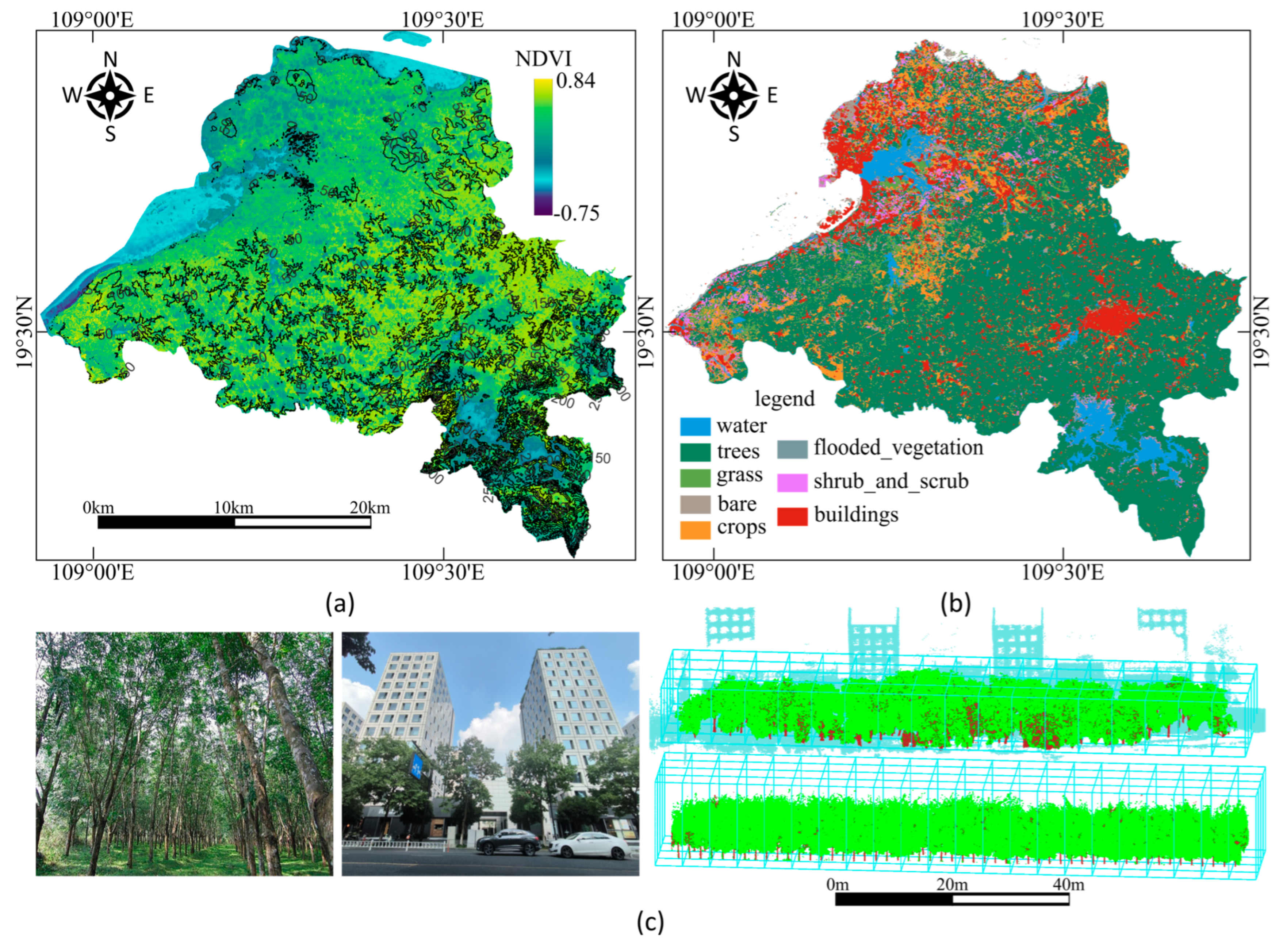
2.1. Study Area and Data Acquisition

The study sites were located in Danzhou, Hainan Island, China, due to the prevalence of plantation and mixed forests in this region, which offer a diverse range of canopy structures and levels of coverage. Danzhou is situated within the low-latitude tropics and experiences a tropical monsoon climate. The annual average temperature is 23.5 °C, with temperatures ranging from 17.5 °C to 27.8 °C. The average annual precipitation is 1815 mm, with above-average sunshine hours, providing suitable conditions for various tree species. A detailed overview of Danzhou is depicted in Figure 1, including the normalized difference vegetation index (NDVI), contour lines, and topographic features.

Terrestrial LiDAR scanning (TLS) was conducted on mild days with a Leica C10 Scanstation. The dates were 15 August 2019 and 13 November 2022. The scanning parameters were set as follows: scan angle, 360° (horizontal) × 270° (vertical); scan rate, 50,000 points/s; angular accuracy, medium at 0.057° (both horizontal and vertical). Multistation scanning was performed to minimize shading effects, with an average distance of 3 m between the stem center and each station. The average point density was approximately 12,000 points/m².

2.2. Data Preprocessing and Dataset Construction

Median filtering [27] was applied to reduce noise by replacing each point in the point cloud with the median of its neighboring points, effectively removing isolated outliers while preserving the local geometry. To remove ground points, the Cloth Simulation Filter (CSF) [28] was employed. This filter simulates a cloth surface that drapes over the point cloud, distinguishing ground points from non-ground points by leveraging the natural deformations in the cloth model. Individual tree segmentation [29] was performed to reduce the data volume, isolating each tree from the surrounding environment for more focused processing. Following segmentation, the segmented point clouds were normalized to a standard range, compressing the data volume while preserving essential morphological features. This normalization step ensures that the relative spatial relationships between points are maintained, allowing the network to learn meaningful representations from the data.

In the dataset annotation process for accurate leaf and wood component separation, we initially applied an automated segmentation method based on machine vision [30]. However, when errors in classification were visually apparent to the human annotators (e.g., due to occlusion, noise, or ambiguous point cloud data), manual corrections were applied. This manual intervention occurred specifically when the model’s predictions conflicted with the expected results, particularly in complex or challenging cases where automated methods were less reliable. This manual intervention occurred when specific criteria were met. These criteria included: (1) cases where the IoU (intersection over union) for either branches or leaves of a particular tree fell below 80%, indicating a significant mismatch between predicted and ground-truth labels; or (2) instances where visual inspection clearly showed branches being misclassified as leaves or leaves being misclassified as branches.

The prepared dataset encompasses three distinct LiDAR point cloud collections, each featuring a different forest type: a rubber tree plantation with Hevea brasiliensis (Willd. ex A. Juss.) Müll. Arg. aged for 5, 10, or 20 years; a mixed forest primarily composed of Litsea glutinosa (Lour.) C.B. Rob., Acacia auriculiformis A. Cunn. ex Benth., and Streblus asper Lour.; and an urban forest populated with the same rubber tree species. Additionally, to ensure a more rigorous evaluation of the proposed method and address concerns regarding scalability and potential subjectivity in manual correction, we integrated two publicly available datasets: LeWoS [31], which includes point cloud data from tropical tree species with varied canopy structures, and a subset of Treenet3D [32], a synthetic dataset focused on rubber trees with uniform structure and density. Both datasets come with comprehensive ground-truth labels, ensuring their suitability for validating the proposed method. This allowed us to assess the network’s generalization capabilities across different tree species and conditions. For testing purposes, 30% of the data are utilized, while 70% are allocated for training.

Table 1. Prepared dataset for deep learning.

	Private Dataset			Public Dataset
	Rubber Tree Plantations	Mixed Forest	Urban Forest	LeWoS	TreeNet3D (Flamboyant Tree)
Type	TLS	TLS	ALS	TLS	Synthetic
Age (Years)	10	15	10	-	-
Quantity (Training / Test)	285/122	167/70	66/28	43/18	490/210
Avg. Height (m)	9.72	11.65	11.86	33.7	133.19
Avg. Diameter at Breast Height (cm)	16.7	23.46	31.08	58.4	359
Avg. Crown Width (m) (N–S)/ (E–W)	2.91/3.74	3.05/3.11	6.82/7.12	14.0/14.57	102.89/104.03
Density (m)	0.02	0.13	0.06	0.05	0.01
Data Size (GB)	10.8	1.2	0.4	10.4	47.6

presents the specific statistics of the prepared dataset. The tree height and crown diameter were calculated by determining the differences between the maximum and minimum coordinate values along the three spatial axes. The diameter at breast height (DBH) was measured using Circular Hough Transform [33] on a cross-section at approximately 1.3 m above the ground.

3. Segmentation Network

The enhanced Point Transformer (PT) network for wood–leaf separation consists of the following components, as shown in Figure 2. Initially, the point clouds of individual trees were sparsely sampled using farthest-point sampling (FPS, light red block in Figure 2) [34], reducing the complexity to 4096 points. The FPS process is as follows:

• Randomly select an initial point: Start by randomly choosing a point from the point cloud as the first point in the sampled set.
• Calculate distances: For each remaining point in the point cloud, calculate the distance to the nearest point in the already selected set of points.
• Select the farthest point: Choose the point with the maximum distance from the points already selected. This point is then added to the set of sampled points.
• Repeat until the desired number of points is reached: Continue steps 2 and 3 until the desired number of points (in this case, 4096) has been selected. This ensures that the points are evenly distributed and well represent the structure of the original point cloud.

The FPS algorithm has a computational complexity of $O\left(n·m\right)$, where $n$ is the number of original points in the cloud, and $m$ is the number of sampled points (4096 in this study).

Next, the features of these points were computed through the Local Surface Features Extraction (LSFE) module. The features $F^{in}$ and coordinates $P^{in}$ of these points were fed into the network for training. The network allows each stage in the decoder to take the output of the previous layer and the output of the corresponding layer in the encoder as input to exhibit a symmetrical encoder–decoder structure. More specifically, the architecture unfolds across five phases in the encoder stage. The initial phase incorporates Multilayer Perceptron (MLP, green–yellow block in Figure 2) and a Point Transformer Block (PTB, light pink block in Figure 2). Subsequently, the encoder seamlessly progresses through four consecutive phases, each comprising feature abstraction (FA, lime yellow block in Figure 2) prior to a subsequent PTB. Transitioning to the decoder stage involves five upsampling steps, starting with an MLP and Feature Propagation (FP, light grey block in Figure 2). After this initial step, the process includes four additional steps, each consisting of FP followed by a PTB module. This orchestrated sequence gradually reinstates global features and enhances the overall semantic segmentation performance. The final logits for each point are obtained by applying an MLP layer to the output, which converts the features into semantic segmentation labels.

3.1. Local Surface Features Extraction (LSFE)

Three-dimensional point cloud networks typically take the raw 3D coordinates of points as input, sometimes including surface normals, and extract and encode class-specific attributes from these raw data. However, 3D point cloud networks are still continuously improving their methods of organizing local geometric data. To enhance the informational value of the raw point coordinates, hand-crafted Local Surface Features can be incorporated as additional input attributes. This way, the networks can leverage this extra information to more effectively encode and aggregate the interactions of local structures at various scales.

Therefore, the feature $f_i^{in}\in {ℝ}^{1\times 9},f_i^{in}\in F^{in}$ of each point $p_i^{in}=\left[x_i^{in},y_i^{in},z_i^{in}\right]\in P^{in}$ in the dataset not only includes the 3D coordinates $p_i^{in}=\left[x_i^{in},y_i^{in},z_i^{in}\right]$ and normal vector ${\overrightarrow{n}}_i=\left[n_i^x,n_i^y,n_i^z\right]$, but also incorporates Local Surface Features. This paper introduces Point Feature Histograms (PFH) [35] to define Local Surface Features. For each point $p_i^{in}$, we identify the $\nu$ nearest neighboring points $p_j^i$, $j=1,2,\dots ,\nu$. Herein $\nu =10$, balancing the need to capture local geometric variations in both smooth trunk regions and irregular leaf surfaces while ensuring computational efficiency. First, for each pair $p_i^{in}$ and $p_j^i$, we establish a local coordinate system to normalize the orientation of neighboring points, ensuring consistent feature extraction that is invariant to the global coordinate system, as follows:

$$\begin{array}{c}{u}_{i,j}={\overrightarrow{n}}_i\hfill \\ v_{i,j}=u_{i,j}\times {\displaystyle \frac{\left(p_i^{in}-p_j^i\right)}{d_{i,j}^2}}\hfill \\ w_{i,j}=u_{i,j}\times v_{i,j}\hfill \end{array}$$

(1)

In these equations, $\times$ represents the cross product, ${\overrightarrow{n}}_i$ denotes the normal vector of $p_i^{in}$, and $d_{i,j}=\parallel p_i^{in}-p_j^i\parallel$. Notably, for each $p_j^i$, $u_{i,j}$ is assigned the normal vector of $p_i^{in}$.

Next, we compute the following three features:

$$\begin{array}{c}{\alpha }_{i,j}=v_{i,j}\cdot {\overrightarrow{n}}_j^i\hfill \\ {\varphi }_{i,j}=u_{i,j}\cdot {\displaystyle \frac{\left(p_j^i-p_i^{in}\right)}{d_{i,j}}}\hfill \\ {\theta }_{i,j}=\mathit{arctan}2\left(w_{i,j}\cdot {\overrightarrow{n}}_j^i,u_{i,j}\cdot {\overrightarrow{n}}_j^i\right)\hfill \end{array}$$

(2)

where $\mathit{arctan}2\left(x,y\right)$ is a two-parameter tangent function used to calculate the polar coordinate angle from the positive x-axis to the point $\left(x,y\right)$.

For these 10 neighboring points, we obtain 10 three-dimensional feature vectors, namely $\left[{\alpha }_{i,j},{\varphi }_{i,j},{\theta }_{i,j}\right]\in {ℝ}^{1\times 3}$. We concatenate these 10 vectors vertically to constituting the matrix presented as $PFH\left(p_i^{in}\right)=\left[{\alpha }_{i,1},{\varphi }_{i,1},{\theta }_{i,1};{\alpha }_{i,2},{\varphi }_{i,2},{\theta }_{i,2};\dots ;{\alpha }_{i,10},{\varphi }_{i,10},{\theta }_{i,10}\right]\in {ℝ}^{10\times 3}$.

Next, we refer to the Fast PFH (FPFH) [36] descriptor to improve computational efficiency, as follows:

$$FPFH\left(p_i^{in}\right)=PFH\left(p_i^{in}\right)+{\displaystyle \frac{1}{\nu }}{\displaystyle \sum }_{j=1}^{\nu }{\displaystyle \frac{1}{d_{i,j}}}\cdot PFH\left(p_j^i\right)$$

(3)

where $PFH\left(p_j^i\right)$ is derived similarly for point $p_j^i$.

This step combines the local features of a point with its neighbors’ features, weighted by their distance, to create a more compact and efficient representation.

At this stage, we obtain a matrix consisting of 10 row vectors. For each row vector, we perform the following operation:

$$LSF\left(p_i^{in}\right)={\displaystyle \frac{{\sum }_{j=1}^{\nu }{\mathsf{\omega }}_{i,j}\cdot FPFH{\left(p_i^{in}\right)}_j}{{\sum }_{j=1}^v{\omega }_{i,j}}}$$

(4)

where ${\mathsf{\omega }}_{i,j}={\displaystyle \frac{1}{d_{i,j}}}$, $FPFH{\left(p_i^{in}\right)}_j$ denotes the $j$-th row vector of $FPFH\left(p_i^{in}\right)$, and $LSF\left(p_i^{in}\right)\in {ℝ}^{1\times 3}$.

3.2. Feature Abstraction (FA)

The FA module downsamples the point cloud and extracts local features, which consist of three components: FPS, adaptive shifting, and mixed pooling.

While applied to obtain a sparser subpoint set preserving shape characteristics, FPS suffers from two drawbacks: susceptibility to outliers and constraint to a subset of the original point cloud.

To address these challenges, we introduced adaptive shifting (light cyan block in Figure 2) to refine each point after FPS. The specific operation is as follows. Since the sampled points generated by FPS may be outliers, we performed k-nearest neighbor (kNN, lemon block in Figure 2) analysis to locate $k$ unsampled neighbors $p_j^i$, $j=1,2,\dots ,k$ for each sampled point $p_i$ and simply shifted $p_i$ to the center $p_c={\sum }_{j=1}^k{p}_j^i/k$ of its neighbors. Moreover, we calculated the coordinate difference $p_{c-j}=p_c-p_j^i=\left[x_{c-j},y_{c-j},z_{c-j}\right]$ between $p_c$ and $p_j^i$.

We performed the following steps to pool the feature vectors onto the subset and derive the features of the sampled points after shifting. We weighted each expanded feature by relative positional encoding, as demonstrated in (5).

$$f_{c,j}=\left(\mathrm{Concat}\left(f_i,f_j^i\right)+\mathrm{PosE}\left(p_{c-j}\right)\right)\odot \mathrm{PosE}\left(p_{c-j}\right)$$

(5)

Here, $\mathrm{Concat}\left(\cdot ,\cdot \right)$ combines vectors end-to-end into a single longer vector. $f_i$ and $f_j^i$ are the features of $p_c$ and $p_j^i$, respectively. The symbol $\odot$ represents the Hadamard product, which performs element-wise multiplication between the combined features and the positional encoding. This operation effectively scales each feature dimension by its corresponding positional value, embedding spatial information directly into the feature space. PosE is introduced in the next section.

In the final stage of FA, mixed pooling [37] aggregated the local features of each point in the subset (white block in Figure 2).

3.3. PosE

The PosE, which is shown in Figure 2, comprises trigonometric dimensionality expansion, Random Fourier Feature-based Transformation (RFFT), and an MLP, as follows:

$$\mathrm{PosE}\left(p_{c-j}\right)=\mathrm{MLP}\left(\mathrm{RFFT}\left(T_j\right)\right)=\mathrm{MLP}\left(\mathrm{RFFT}\left(\mathrm{Concat}\left(t_j^x,t_j^y.t_j^z\right)\right)\right)$$

(6)

Herein, RFFT predominantly utilizes the Random Fourier Feature (RFF) to obtain the correlation between two vectors. $t_j^x,t_j^y,t_j^z\in {ℝ}^{48\times 1}$ are the trigonometric expansions of $p_{c-j}=\left[x_{c-j},y_{c-j},z_{c-j}\right]$, and their concatenation into $T_j=\mathrm{Concat}\left(t_j^x,t_j^y,t_j^z\right)\in {ℝ}^{144\times 1}$ enhances the MLPs’ ability to comprehend high-frequency content during the training phase [38]. Specifically, the feature of $t_j^x$ is calculated based on the first component $x_{c-j}$ of $p_{c-j}$ employing trigonometric dimensionality expansion [39], which is represented as:

$$t_j^x\left[m\right]=\mathit{sin}\left(\alpha x_{c-j}/{\beta }^{{\displaystyle \frac{m/2}{24}}}+{\displaystyle \frac{\pi }{2}}\cdot \left(m\mathrm{mod}2\right)\right)$$

(7)

where $t_j^x$ is the calculated subcomponent derived from $x_{c-j}$. $\alpha ,\beta$ control the amplitude and wavelength of the sine function, which are set as 100 and 500 [40], respectively, in this study. $m\in \left\{0,1,2,\dots ,47\right\}$ represents the $m$-th value in $t_j^x$.

$t_j^y$ and $t_j^z$ are calculated by applying the same trigonometric dimensionality expansion with the input of $y_{c-j}$ and $z_{c-j}$, respectively, as was used for $t_j^x$ in (7). Subsequently, we concatenated these components collectively as $T_j=\mathrm{Concat}\left(t_j^x,t_j^y,t_j^z\right)\in {ℝ}^{144\times 1}$.

3.4. RFFT

After obtaining $T_j$, we leveraged RFFT to uncover the intrinsic spatial correlations present in the dataset, as follows:

$$\mathrm{RFFT}\left(T_j\right)=\mathrm{Concat}\left({\displaystyle \sum }_{l=1}^k\left(\kappa \left(T_j,T_l\right)\cdot T_l\right),\mathcal{Z}\left(T_j\right)\right)$$

(8)

In this equation, $l=1,2,\dots ,k$ denotes the index of a specific vector $T_l$. Similar to $T_j$, $T_l$ represents the feature of a neighboring point $p_l^i$ of $p_i$ after trigonometric dimensionality expansion. $\kappa \left(T_j,T_l\right)\approx \mathcal{Z}{\left(T_j\right)}^T\cdot \mathcal{Z}\left(T_l\right)$, which represents the inner product of the vectors mapped by the RFF mapping function $\mathcal{Z}:{ℝ}^{d_1}\to {ℝ}^{d_2}$, is used to estimate the similarity between $T_j$ and $T_l$ in the lower-dimensional Euclidean space ${ℝ}^{d_2}$. The mapping function is as follows:

$$\begin{gathered} \mathcal{Z}\left(T_j\right)=\sqrt{{\displaystyle \frac{2}{d_2}}}\left[\mathit{cos}\left(\mathcal{T}{T}_j+\beta \right)\right] \\ =\sqrt{{\displaystyle \frac{2}{d_2}}}\left[\mathit{cos}\left({\tau }_1^T{T}_j+{\beta }_1\right),\mathit{cos}\left({\tau }_2^T{T}_j+{\beta }_2\right),\right.{\left.\dots ,\mathit{cos}\left({\tau }_{d_2}^T{T}_j+{\beta }_{d_2}\right)\right]}^T \end{gathered}$$

(9)

Within this equation, $d_2=156$ represents the dimensionality of the transformed features after $\mathcal{Z}\left(·\right)$. This choice is made to balance the need for high-dimensional representations in the Feature Aggregation (FA) module, where input feature dimensions increase (32, 64, 128, 256), and the subsequent transformation in the Point Transformer Block (PTB), which operates in a 512-dimensional space. The matrix $\mathcal{T}={\left[{\tau }_1,{\tau }_2,\dots {\tau }_{d_2}\right]}^T\in {ℝ}^{d_2\times d_1}$ is formed by stacking the vectors ${\tau }_{\mathfrak{d}}$ (where $\mathfrak{d}=1,2,\dots ,d_2$) as rows, each of which is drawn independently from a normal distribution $\mathcal{N}\left(0,1\right)$. Each bias term ${\beta }_{\mathfrak{d}}$ (where $\mathfrak{d}=1,2,\dots ,d_2$) in the vector $\beta ={\left[{\beta }_1,{\beta }_2,\dots ,{\beta }_{d_2}\right]}^T\in {ℝ}^{d_2\times 1}$ is independently sampled from a uniform distribution over the interval [0, 2π] [41].

The use of $\mathcal{N}\left(0,1\right)$ for parameter sampling directly corresponds to implementing a Gaussian kernel for the Random Fourier Features (RFF) mapping. Inspired by the advancements in Orthogonal Random Features (ORF), which have introduced innovative strategies for parameter sampling, we implement a Gaussian kernel as the kernel function, which is defined as follows:

$$\kappa \left(T_j,T_l\right)=e^{{\displaystyle \frac{-\parallel T_j-T_l{\parallel }^2}{2{\sigma }^2}}}$$

(10)

By default, $\sigma =1$, consistent with the standard deviation of the normal distribution used to sample ${\tau }_{\mathfrak{d}}$, ensuring that the kernel operates in a normalized feature space. Since $d_2>d_1$, $\mathcal{T}$ can be considered as the result of concatenating multiple independently generated square linear transformation matrices with size of $d_1\times d_1$. To ensure orthogonality, we adopt techniques inspired by Orthogonal Random Features (ORF). Specifically, when $\sigma =1$, each square linear transformation matrix ${\mathcal{T}}^{\prime }\in {ℝ}^{d_1\times d_1}$ can be seen as a random Gaussian matrix, with each entry independently sampled from the standard normal distribution. Since the norms of the rows of ${\mathcal{T}}^{\prime }$ follow the Chi-square distribution, while the rows of an orthogonal matrix have unit norms, ${\mathcal{T}}^{\prime }$ can be replaced with the next equation to impose orthogonality:

$${\mathcal{T}}^{\prime }=SQwhere\begin{array}{c}S=diag\left(s\right),s\sim {\chi }_d\\ Q=orth\left({\mathcal{T}}^{\prime }\right)\end{array}$$

(11)

where $S\in {ℝ}^{d_1\times d_1}$ is a diagonal matrix with its entries independently and identically distributed from a Chi-square distribution with $d_1$ degrees of freedom. $Q\in {ℝ}^{d_1\times d_1}$ is a uniformly distributed random orthogonal matrix generated by performing a QR decomposition on ${\mathcal{T}}^{\prime }$.

3.5. Point Transformer Block

The PTB, whose specific structure is displayed in the thistle box at the right of Figure 2, encodes global features and exploits the point cloud topology. The PTB is a residual block that takes points $p_i^{in}\in P^{in}\in {ℝ}^{n\times 3}$ and their features $f_i^{in}\in F^{in}\in {ℝ}^{n\times c}$ as inputs, where $n$ and $c$ are the number and feature dimension of the input points, respectively. The features were mapped to a higher-dimensional space of size $n$×512 by a linear layer (light orange block in Figure 2). Then, for each point $p_i^{in}$, pointwise operations were performed (red dashed box in Figure 2). The k-nearest neighbors $p_j^i=\left(x_j^i,y_j^i,z_j^i\right)\in P^{in}$ and $j=1,2,3,\dots ,k$ of $p_i^{in}$ were obtained by kNN. The feature vector $f_i^{in}$ was updated to $f_i^{{in}^{\prime }}$ using the feature vector $f_j^i$ of $p_j^i$ as follows:

$$\begin{gathered} f_i^{{in}^{\prime }}={{\displaystyle \sum }}_{p_j^i}\rho \left(\mathrm{MLP}\left(f_i^{in}{W}_1-f_j^i{W}_2+PosE\left(p_{i-j}\right)\right)\right)\odot \left(f_j^i{W}_3+PosE\left(p_{i-j}\right)\right) \\ where{p}_{i-j}=p_i^{in}-p_j^i \end{gathered}$$

(12)

In (12), $W_1$, $W_2$, and $W_3$ are trainable pointwise transformations (light orange blocks in Figure 2, uniform $512\times 512$ size). $\rho$ is a SoftMax function (violet block in Figure 2), weighting the contribution of each neighbor to the central point’s representation. This enables the network to focus on the most relevant neighbors and effectively capture the complex spatial relationships within the dense forest canopy.

At the end of the PTB, a linear layer was used to reduce the feature dimension, followed by a residual connection to obtain the global features as the PTB output.

3.6. Feature Propagation

In the encoder stage, as the network samples fewer points layer by layer to ensure sufficient global information, it becomes impossible to complete the segmentation task. This is because point cloud classification is an end-to-end task that assigns semantic labels to each point, requiring the output to match the input in point number.

To this end, feature propagation modules that performed the inverse operation of FA were added in the decoder stage. This module adopts the transition up from PT, which uses trilinear interpolation to map features from subsets back to supersets. Further details regarding the FP module can be found in [34].

4. Computational Experiments

4.1. Computational Environments

All the laboratory work was processed by a desktop computer. It had an Intel i7-7700 CPU @ 2.80 GHz, 16 GB of RAM, and an NVIDIA RTX 4090 super card. The integrated development environment (IDE) we used for deep learning was PyCharm 2022.2.2 (JetBrains, Prague, Czech Republic).

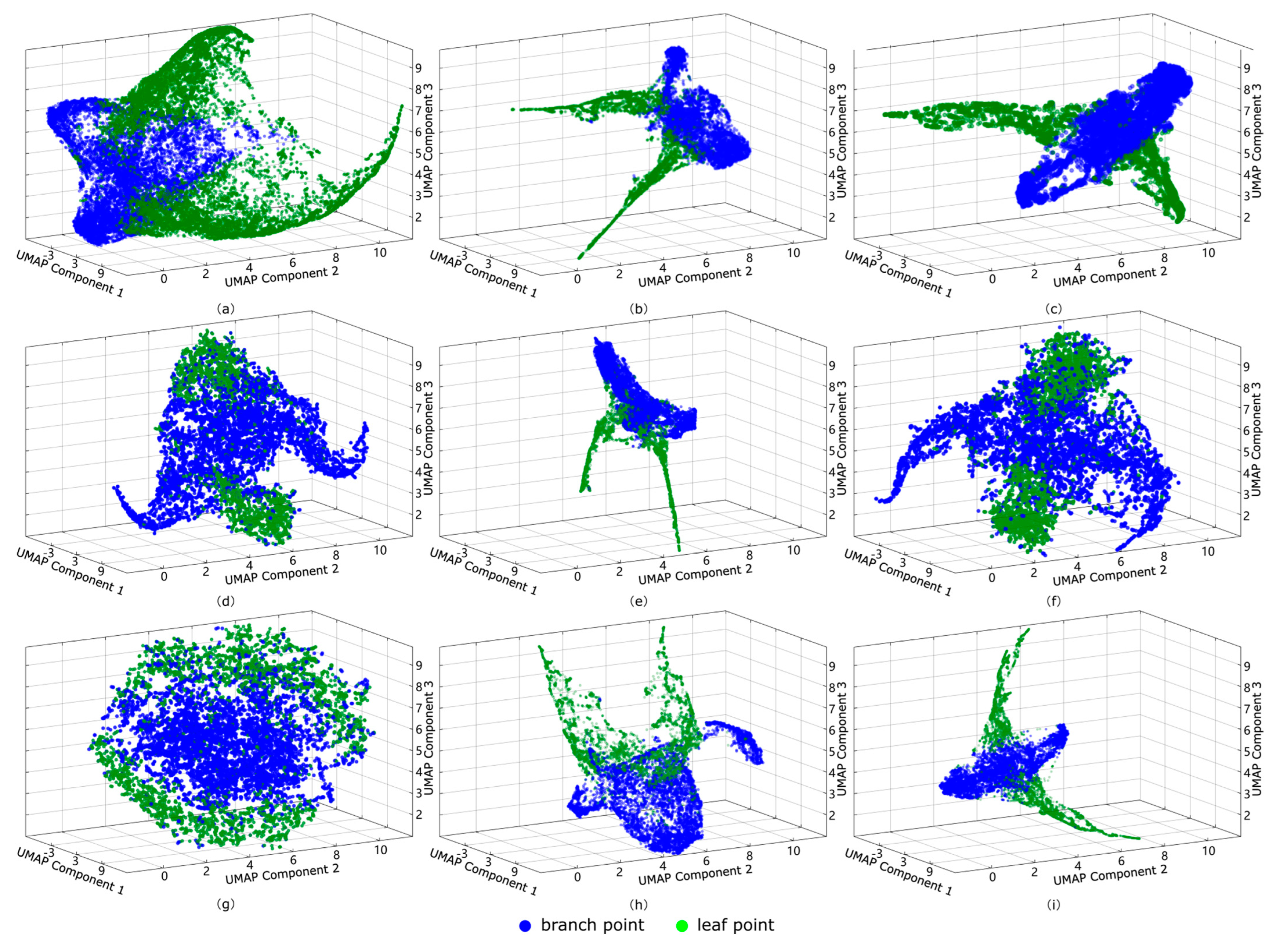
4.2. Local Surface Features

To validate the effectiveness of the proposed LSF in enhanced network, we conducted a visualization analysis using Uniform Manifold Approximation and Projection (UMAP) [42]. UMAP involves four primary steps:

• Constructing the High-Dimensional Graph: UMAP begins by constructing a k-nearest neighbor (kNN) graph in high-dimensional space. For each point $p_i$ in the dataset, the algorithm identifies its k-nearest neighbors. The similarity weight $w_{i,j}$ between each pair of neighboring points $p_i$ and $p_j$ is then calculated as follows:

  $$w_{ij}^{high}=\exp \left(-{\displaystyle \frac{\mathrm{dist}\left(f_i,f_j\right)-{\rho }_i}{{\sigma }_i}}\right)$$

  (13)

Here, $f_i=\left[x_i,y_i,z_i,n_i^x,n_i^y,n_i^z,LSF\left(p_i\right)\right]\in {ℝ}^{1\times 10}$ and $f_j=\left[x_j,y_j,z_j,n_j^x,n_j^y,n_j^z,LSF\left(p_j\right)\right]\in {ℝ}^{1\times 10}$ are the Local Surface Feature vectors of $p_i$ and $p_j$, respectively, with $\mathrm{dist}\left(f_i,f_j\right)$ representing the Euclidean distance between these features. ${\rho }_i$ denotes the distance from $f_i$ to its closest neighbor in the kNN graph, adjusting for local density, while ${\sigma }_i$ is a tuning parameter that ensures an appropriate similarity value across different density regions. Notably, the symbols $f_i,f_j,p_i$, and $p_j$ here are not related to those in Chapter 3.

2.

Constructing the Low-Dimensional Graph: In the low-dimensional space, UMAP initializes a graph structure and calculates similarity weights for each pair of points in a manner similar to the high-dimensional graph. The goal is to maintain the local similarity relationships found in the high-dimensional space within the low-dimensional structure. The calculation is as follows:

$$w_{ij}^{low}={\displaystyle \frac{1}{1+a·\mathrm{dist}{\left(f_i^{low},f_j^{low}\right)}^{2b}}}$$

(14)

In this equation, $f_i^{low}$ and $f_j^{low}$ are the low-dimensional representations of $f_i{f}_j$, respectively.

3.

Optimizing the Low-Dimensional Embedding: UMAP optimizes the low-dimensional embedding by minimizing the difference between the high-dimensional and low-dimensional graphs. Specifically, it seeks to find the optimal set of low-dimensional feature vectors $F^{low}$. The objective function for this optimization is typically defined using cross-entropy loss as follows:

$$L={\displaystyle \sum }_{p_i\ne p_j}\left[w_{ij}^{high}\log \left({\displaystyle \frac{w_{ij}^{high}}{w_{ij}^{low}}}\right)+\left(1-w_{ij}^{high}\right)\log \left({\displaystyle \frac{1-w_{ij}^{high}}{1-w_{ij}^{low}}}\right)\right]$$

(15)

By minimizing this loss function, UMAP adjusts the set of low-dimensional feature vectors $F^{low}$ to best preserve the high-dimensional local structure in the low-dimensional embedding.

4.

Projection and Visualization: After optimization, the resulting low-dimensional feature are mapped onto the axes (e.g., Component 1, Component 2, and Component 3) for three-dimensional visualization, preserving the data’s local structure and distributional characteristics.

The 3D visualization of Local Surface Features is as illustrated in Figure 3. The results clearly demonstrate that UMAP successfully separates the two classes of points, even when only Local Surface Features Extraction is applied. This observation indicates that the selected features perform excellently in distinguishing between different categories of data, thereby reflecting the inherent structure and characteristics of the data. This finding not only supports our hypothesis but also provides a theoretical basis for the subsequent training and optimization of the model.

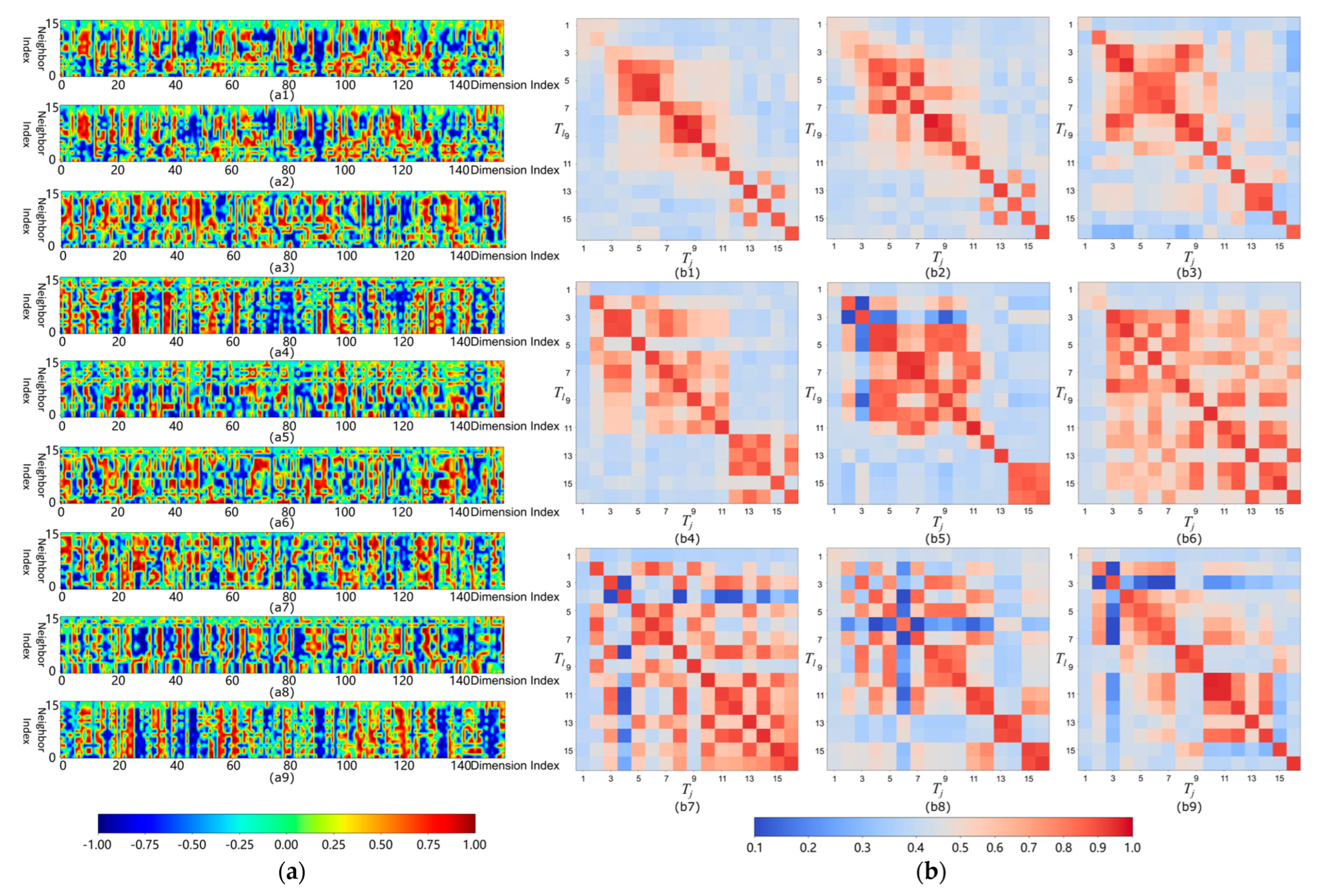
4.3. Results of RFFT

Figure 4 shows the outcomes from RFFT. In this figure, a point was randomly selected with its 16 neighbors to calculate the interpoint covariance $\kappa \left(T_j,T_l\right)$, showcasing 16 neighbors’ features after $Z\left(\cdot \right)$. Notably, the 156-dimensional feature values derived from $Z\left(\cdot \right)$ inject substantial complexity into the dataset, enhancing the neural network’s capability to discern intricate patterns and capture unique frequency attributes. This enriched representation enables the neural network to capture subtle variations and intricate structures, significantly improving its ability to generalize and perform on the wood–leaf separation task. The non-linearities introduced by $Z\left(\cdot \right)$ empower the network to adapt to complex datasets, thereby enhancing its learning efficiency and overall performance. To more intuitively reveal relationships among neighboring points through feature correlations, panel (b) illustrates the inter-point correlation $\kappa \left(T_j,T_l\right)$ within neighborhoods.

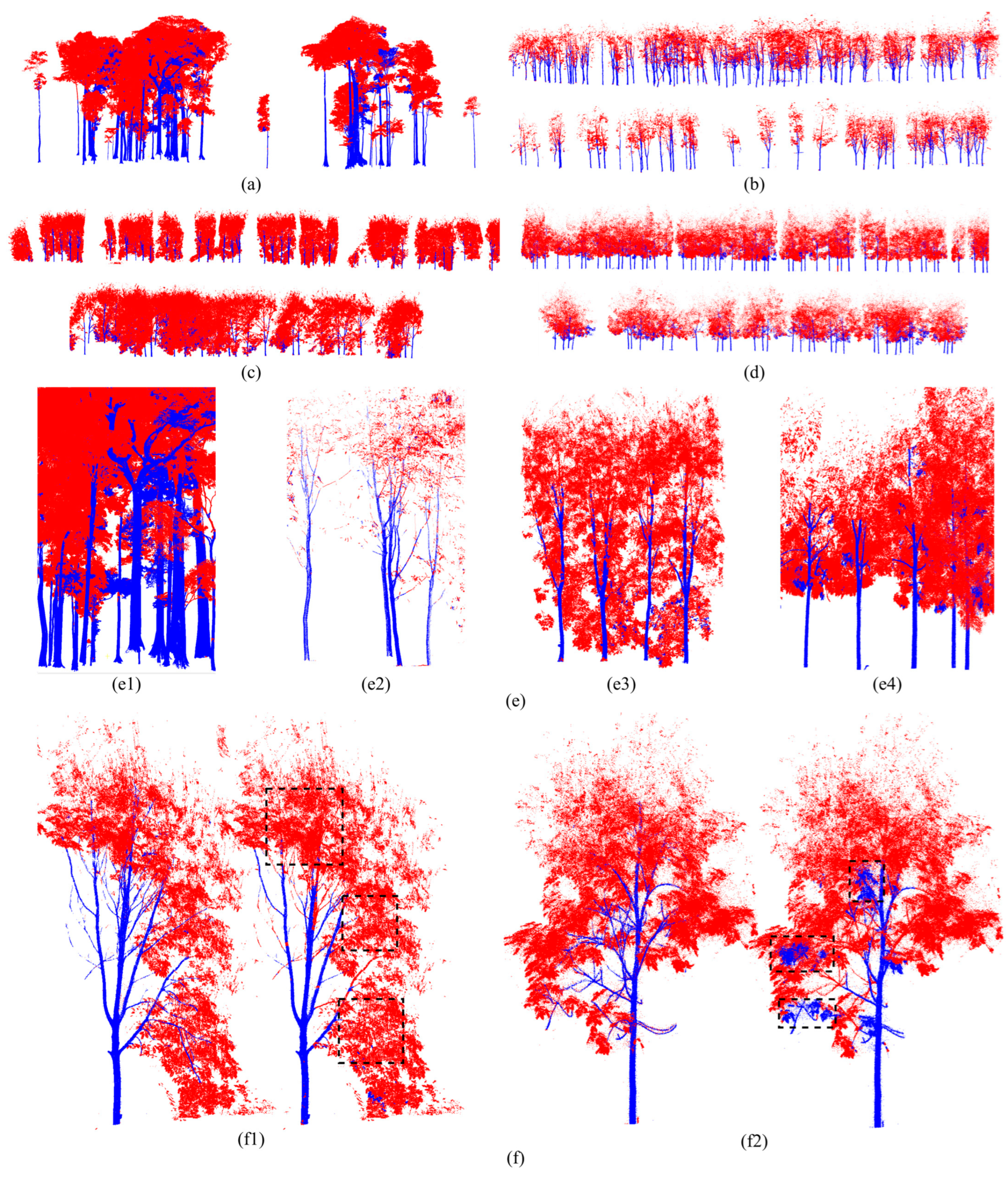
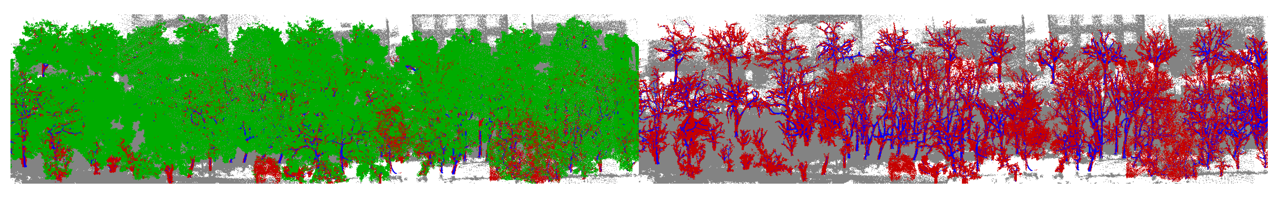
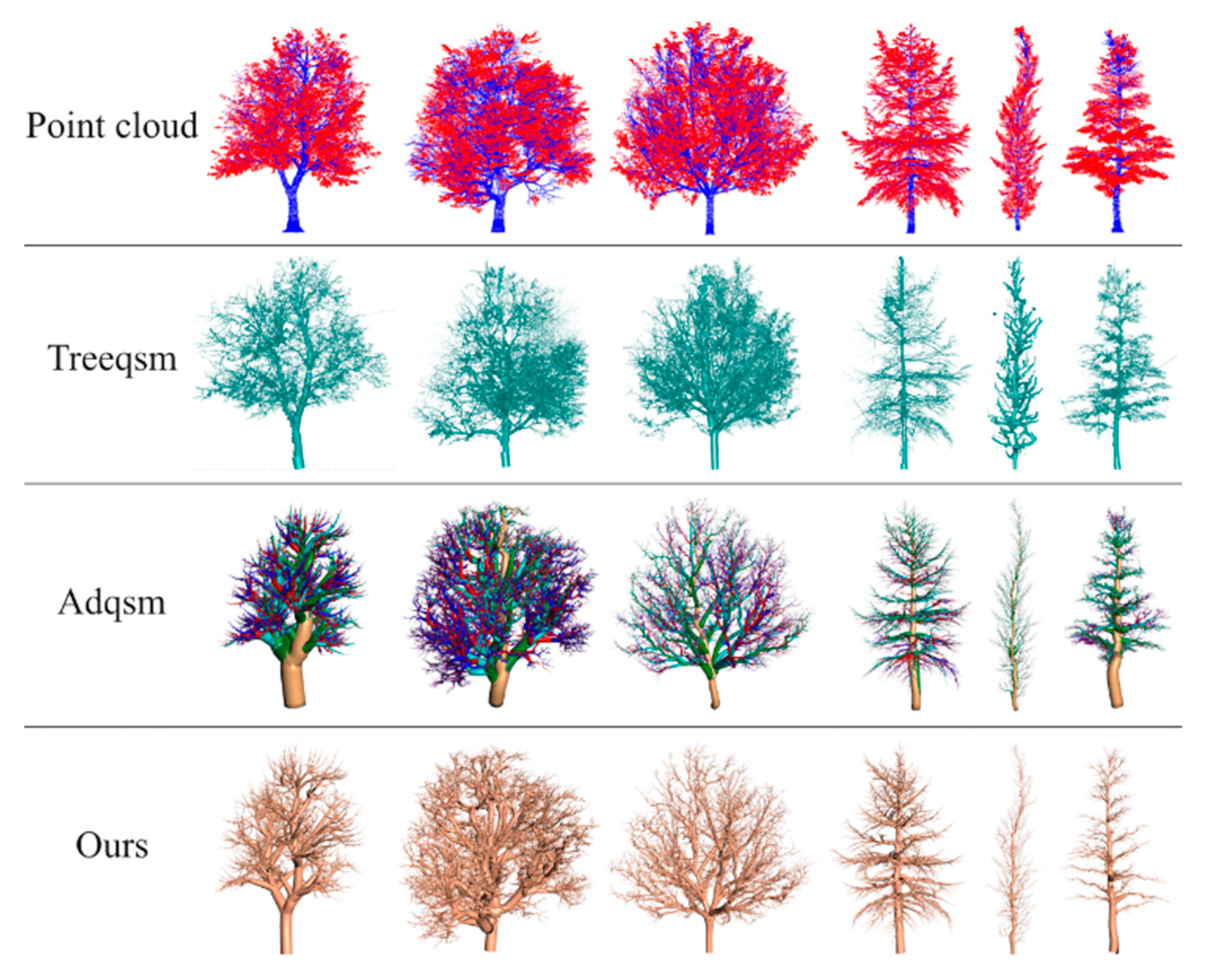
4.4. Wood–Leaf Separation

The training course lasted approximately 9.5 h. Each input consisted of 4096 points with an initial learning rate of 0.0015, a weight decay of 0.0004, a learning rate decay of 0.8, a batch size of 2, and 200 iterations. Meanwhile, AdamW optimizer [43] was used as optimizer in this experiment. In kNN, $k$ was set to 16 for feature abstraction and 3 for FP [26]. All hyperparameter settings are listed in Appendix A.

In Figure 5, the partial wood–leaf segmentation results of the test set are presented. While the model effectively distinguishes branch points from leaf points overall, some misclassifications are observed. Branch points in the canopy were occasionally misclassified as leaf points, and conversely, some leaf points were misclassified as branch points. These errors, influenced by factors such as occlusion, contribute to a reduction in accuracy. However, the results demonstrate the model’s strong ability to separate wood and leaf points effectively in most cases.

4.5. Ablation Studies

This study performs ablation experiments to thoroughly validate the effectiveness of the proposed Local Surface Features and PosE. Specifically, in our ablation experiments, when Local Surface Features are excluded, the input features consist solely of the coordinates and normals of the points. Furthermore, in scenarios where PosE is not applied, it is substituted with relative positional encoding for comparative purposes. The experimental results are summarized in

Table 2. Ablation experiment results for Local Surface Features and PosE.

Local Surface Features	PosE (in FA)	PosE (in PTB)	NPTB	Precision (%)	mIoU (%)	Time (s/per Tree)
×	×	×	10	87.31	79.07	2.90
×	√	×	10	89.01	81.27	3.25
×	×	√	10	89.14	81.35	3.28
×	√	√	10	91.13	82.77	4.07
√	×	×	10	89.21	81.52	3.32
√	√	×	10	91.34	83.00	4.08
√	×	√	10	91.52	83.32	3.99
√	√	√	6	91.06	83.01	3.86
√	√	√	8	92.59	83.81	4.30
√	√	√	12	92.62	83.93	5.17
√	√	√	14	91.35	81.80	5.68
√	√	√	10	94.36	85.48	4.62

NPTB denotes the number of PTBs. The symbol “×” indicates that a specific module is not used, while “√” signifies that the module is used.

. The data in the table reveal several key findings. Examining the performance differences of PTB with and without PosE, it is evident that the model’s performance significantly improves when PosE is integrated into the original attention mechanism. This improvement is attributed to PosE’s ability not only to capture the coordinate differences between two points but also to integrate richer positional information, thereby enhancing the model’s understanding of spatial relationships.

When PosE was introduced in FA, we found that the sampling points can better integrate and more effectively express the originally complex and hard-to-capture local geometric information. This indicates that PosE plays a crucial role in promoting feature fusion and enhancing local feature expression capabilities. Further analysis reveals that, in the absence of Local Surface Features, the model’s precision and mIoU significantly increase by 3.82% and 3.7%, respectively, when both the FA and PTB modules utilize PosE, compared to when neither module employs PosE. This significant performance improvement fully demonstrates the synergistic effect of PosE in the two modules, indicating that they jointly leverage positional information to more comprehensively understand the spatial structure and contextual relationships of point cloud data, thus achieving more precise segmentation or recognition tasks.

Moreover, the inclusion of Local Surface Features also shows noticeable performance enhancements. When Local Surface Features are combined with PosE in the FA and PTB modules, there is a further increase in precision by 7.05% and mIoU by 6.41%, indicating that Local Surface Features provide additional contextual and geometric information that aids in the model’s performance.

The study also explores the impact of varying the number of Point Transformer Blocks (NPTB) on the performance of the proposed model. Specifically, in our ablation experiments, we tested different configurations of NPTB while incorporating or excluding PosE and Local Surface Features. The data demonstrate that when NPTB is set to 10, and both Local Surface Features and PosE are enabled in the Feature Aggregation (FA) and Point Transformer Block (PTB) modules, the model achieves the highest precision of 94.36% and an mIoU of 85.48%. This configuration highlights the synergistic effect of combining PosE with Local Surface Features, as well as the importance of carefully selecting the number of PTBs to optimize performance. Furthermore, varying NPTB shows that while a decrease in the number of blocks (e.g., NPTB = 6 or 8) leads to slightly lower performance, increasing the number beyond 10 does not necessarily result in significant improvements and may even lead to diminishing returns. For instance, when NPTB is set to 12 or 14, precision and mIoU do not surpass the results achieved with 10 blocks.

From a time–cost perspective, the enhanced PT network takes an additional 1.72 s per tree compared to the original PT network. However, this extra time is justified by a significant improvement of nearly 6% in mIoU. The increased computational cost is outweighed by the enhanced segmentation accuracy, demonstrating that the additional processing time is a worthwhile trade-off for the performance gain.

To further investigate the efficiency of PosE, we conducted an ablation study on the position encoding methods, as shown in

Table 3. Ablation experiment results for position encoding.

Position Encoding	Precision (%)	mIoU (%)	Time (s/per Tree)
none	83.02	76.29	2.76
absolute	85.34	78.67	2.89
relative	89.21	81.52	3.32
relative for attention	86.17	78.60	3.36
relative for feature	87.44	79.65	3.93
PosE	94.36	85.48	4.62

. The formulas for the absolute position encoding $e_i^{ab}$, relative position encoding $e_{i,j}^{re}$, relative for attention $e_{i,j}^{refa}$, and relative for feature $e_{i,j}^{reff}$ are as follows:

$$e_i^{ab}=W^{ab}{p}_i$$

(16)

$$e_{i,j}^{re}=W^{re}\parallel p_i-p_j\parallel$$

(17)

$$e_{i,j}^{refa}=Softmax\left({\displaystyle \frac{{\left(W_i^{refa}{p}_i\right)}^T{W}_j^{refa}{p}_j+e_{i,j}^{re}}{\sqrt{d_k}}}\right)$$

(18)

$$e_{i,j}^{reff}=f_i+W^{reff}\parallel p_i-p_j\parallel$$

(19)

where $W^{ab}$, $W^{re}$, $W_i^{refa}$, and $W_j^{refa}$ are linear layers of size 512, and $W^{reff}$ is a linear layer with the same dimensionality as $f_i$. $d_k$ is set to 512.

The results presented in Table 3 demonstrate the impact of different position encoding methods on model performance and computational efficiency. Among all methods, PosE achieves the highest precision (94.36%) and mIoU (85.48%), significantly outperforming other position encodings. This improvement, however, comes with a higher computational cost, requiring 4.62 s per tree, reflecting the additional complexity of its enhanced positional encoding mechanism. In contrast, the relative position encoding achieves a balance between performance (89.21% precision, 81.52% mIoU) and efficiency (3.32 s per tree), while simpler encodings, such as absolute position encoding, offer faster computations (2.89 s per tree) but relatively lower performance. The relative-for-feature and relative-for-attention encodings provide moderate performance improvements over the absolute encoding but introduce slightly higher computational costs. These results highlight PosE’s advantage in achieving superior accuracy and segmentation quality, which is particularly beneficial for tasks requiring high precision, despite its computational overhead.

4.6. Comparison with Existing Methods

As shown in

Table 4. Comparison of the separation performance across different methods.

		Rubber Tree Plantations	Mixed Forest	Urban Forest	LeWoS	TreeNet3D
Machine learning [30]	Precision (%)	84.94	71.01	85.02	85.87	86.47
	mIoU (%)	74.01	63.69	75.31	75.92	77.86
PointNet++ [21]	Precision (%)	86.34	71.99	87.33	87.83	88.23
	mIoU (%)	75.96	65.19	77.43	78.21	80.19
PSegNet [20]	Precision (%)	89.97	75.81	90.23	90.79	91.97
	mIoU (%)	80.69	69.19	82.99	83.27	85.01
PT [26]	Precision (%)	89.71	75.00	89.91	90.26	91.70
	mIoU (%)	80.99	68.92	81.31	82.94	85.00
RepSurf-U [44]	Precision (%)	89.22	74.43	89.24	89.95	91.33
	mIoU (%)	79.01	66.94	79.01	79.50	84.75
PointNeXt [22]	Precision (%)	89.50	74.81	89.65	90.41	91.58
	mIoU (%)	80.97	68.89	81.32	81.79	83.06
PointMLP + TAP [45]	Precision (%)	92.11	78.09	91.55	91.90	92.44
	mIoU (%)	84.41	71.26	84.52	84.93	86.07
Point2vec [46]	Precision (%)	89.47	74.69	89.60	90.71	92.06
	mIoU (%)	80.66	68.48	81.00	82.85	85.77
Enhanced PT	Precision (%)	94.69	80.43	94.88	95.31	96.23
	mIoU (%)	86.65	73.51	86.76	87.02	91.51

, our proposed method demonstrates significant advantages over existing approaches across various forest types. Within the private datasets, the network achieves its highest performance on the urban forest dataset, with a precision of 94.88% and an mIoU of 86.76%. This strong result reflects the distinct structural characteristics of urban forests, which typically exhibit fewer occlusions and more standardized branching patterns due to consistent maintenance practices. In contrast, mixed forests present a more complex challenge due to their irregular growth patterns, considerable species diversity, pronounced occlusions, and lower point density, all of which make it difficult to segment individual tree components accurately. Nevertheless, our enhanced PT network achieves a precision of 80.43% and an mIoU of 73.51%, illustrating its adaptability to the high variability and complexity of natural forest structures. Meanwhile, rubber tree plantations, with their uniform and consistent structure, may simplify segmentation. However, the limited structural diversity can reduce opportunities for refining segmentation. Despite this, the network achieves a precision of 94.69% and an mIoU of 86.65%, further indicating its flexibility across different forest environments. On the two publicly available datasets, LeWoS and TreeNet3D, the proposed method produces results that exceed our expectations, with mIoU scores of 87.02% and 91.51%, respectively. Notably, the samples in LeWoS are the least represented within our dataset, emphasizing the robustness of our approach in maintaining high accuracy even with limited data availability. This outcome further demonstrates the network’s robustness against variations in tree species diversity within the datasets. Additionally, our enhanced PT network consistently surpasses the baseline PT model, achieving an approximate 5–6% improvement in both precision and mIoU. These enhancements underscore the effectiveness of our modifications in significantly improving segmentation accuracy.

Since the datasets consist of individually segmented trees, the potential impact of tree density on segmentation accuracy was not directly considered. However, a small number of imperfectly segmented trees within the datasets suggest that the network remains effective across varying tree densities, demonstrating resilience to minor inconsistencies. These results collectively affirm our method’s adaptability and performance across both clearly defined and more complex forest scenarios, showing promising accuracy under varied conditions.

5. Discussion

5.1. Collaborative Synergy Between LSF and PosE: A Paradigm Shift in Wood–Leaf Separation

The proposed method stands apart from traditional wood–leaf separation techniques by uniting Local Surface Features (LSF) and Position Encoding (PosE) in a synergistic framework. This collaboration offers a distinctive advantage in addressing the nuanced spatial and geometric relationships within tree point clouds, overcoming limitations inherent in prior methods that rely predominantly on either geometric features or spatial encoding alone.

The essence of this distinction lies in the complementary roles of LSF and PosE. LSF excels at capturing fine-grained geometric distinctions, leveraging local coordinate systems to normalize the orientation of points and extract features that highlight differences in relative spatial arrangement. These features are explicitly designed to differentiate wood, with its uniform and regular structure, from leaves, which exhibit greater curvature and variability. By anchoring these features to the normal vectors of points, LSF ensures that the geometric representation is invariant to global transformations, a crucial requirement for the diverse orientations encountered in natural forests. On the other hand, PosE provides a robust mechanism for encoding spatial relationships at varying scales. Through trigonometric expansions and Random Fourier Feature-based Transformations (RFFT), PosE captures both local and global spatial hierarchies. This dual capability is particularly vital for distinguishing closely packed leaves from the more sparsely distributed wood components, as well as for resolving occlusions in dense canopies. Furthermore, the sensitivity of PosE to small positional variations allows the model to encode the subtle spatial interdependencies that often delineate wood from leaf regions.

The interplay between LSF and PosE fosters a hierarchical understanding of point cloud data, where LSF delivers localized geometric insights and PosE contextualizes these insights within the broader spatial structure. This collaboration not only enhances segmentation accuracy but also equips the model to generalize across diverse datasets with varying tree species, canopy densities, and levels of occlusion. For instance, experimental results reveal that this approach consistently outperforms state-of-the-art methods in both plantation and mixed forest environments, demonstrating its adaptability to heterogeneous conditions.

In contrast to conventional approaches that either emphasize global geometric patterns or rely on generic position encodings, our method achieves a delicate balance by integrating feature-rich geometry with adaptable spatial encoding. This dual emphasis represents a paradigm shift in wood–leaf separation, moving beyond isolated feature extraction to a more holistic representation of tree point clouds. By combining LSF’s geometric precision with PosE’s spatial robustness, this method establishes a new standard for effectively disentangling the intricate structures of natural forests.

5.2. Design Principles of Local Surface Features

In LSF, we use local coordinate systems to represent the relationship between a point and its neighboring points. The key reason for this approach is to normalize the orientation of points and ensure that the local structure of each point is invariant to global transformations. This is particularly important for forest data, where the orientation and shape of trees can vary significantly, but the relative relationships between neighboring points are crucial for tasks such as segmentation and classification. By attaching a local coordinate system to each point, we can better capture the local geometric structure and ensure that features are consistently represented, regardless of the global position or orientation of the object in the scene. This is achieved by aligning the local coordinate system with the normal vector of the point, which reflects the local surface orientation. In this way, we preserve the local geometry while making the feature representation more robust to transformations such as rotations and translations.

Based on the constructed local coordinate system, we defined three features as presented in Equation (2). Each of these features conveys a distinct meaning: ${\alpha }_{i,j}$ represents the alignment between the relative position (represented by vector $v_{i,j}$) of points $p_i^{in}$ and $p_j^i$, and the normal of point $p_j^i$. It helps distinguish wood from leaves, as wood and leaves usually exhibit different geometric structures and surface features, leading to different normal-relative position differences. ${\varphi }_{i,j}$ calculates the alignment between the normal vector ${\overrightarrow{n}}_i$ of point $p_i^{in}$ and the relative position between $p_j^i$ and $p_i^{in}$. For wood and leaves, leaves often show larger surface curvature and irregular spatial distributions, which ${\varphi }_{i,j}$ helps capture. ${\theta }_{i,j}$ is computed using a combination of vectors $w_{i,j}$ and $u_{i,j}$. It captures the spatial angle between the two vectors, which is crucial for distinguishing wood and leaf points, especially when their surface shapes and spatial distributions differ significantly.

Wood and leaves exhibit significant structural differences: wood typically has a more uniform texture and regular shapes, while leaves tend to have more curvature and irregularities. The geometric features derived from the relationships between points help capture these structural differences. For example, the surface of wood is relatively flat with consistent normal vectors, while leaves have more curvature and complex morphology. In point cloud segmentation, these geometric features help differentiate between local geometries, providing the model with sufficient information to distinguish between various point types. Thus, these features play a critical role in feature representation, particularly when dealing with tree point clouds that exhibit substantial shape differences.

5.3. Discussion on the Effectiveness of PosE

The proposed Position Encoding (PosE) mechanism is designed to enhance the model’s ability to capture spatial relationships within point cloud data. This effectiveness can be attributed to several key aspects of its design. First, the use of trigonometric dimensionality expansion transforms low-dimensional input coordinates into higher-dimensional sinusoidal features. This process enables the MLP to learn high-frequency content during training, which is particularly crucial for modeling fine-grained details in spatial relationships [40]. The sinusoidal mapping ensures that even small variations in point positions are represented distinctly in the feature space, allowing the model to differentiate subtle structural patterns. Second, the integration of Random Fourier Feature-based Transformation (RFFT) further refines these representations by approximating kernel functions, such as the Gaussian kernel, in a lower-dimensional space. This operation efficiently captures pairwise correlations between points while maintaining computational feasibility. The orthogonalization of random matrices in RFFT contributes to stable feature transformations, avoiding the pitfalls of overfitting and ensuring that the encoded spatial relationships are robust across different datasets. Finally, the concatenation of trigonometric expansions for all three spatial dimensions enhances the model’s ability to jointly consider spatial features across axes. This comprehensive representation of spatial correlations is critical in point cloud segmentation tasks, where positional interdependencies often define class boundaries.

Empirical results across diverse datasets, such as LeWoS and TreeNet3D, further validate PosE’s robustness. The significant improvement in performance metrics, particularly in environments with varied density and species heterogeneity, underscores its adaptability. By addressing these challenges, PosE demonstrates its potential as a generalizable solution for spatial encoding in point cloud processing.

Moreover, the selection of $\sigma$ can significantly impact the segmentation results, particularly in terms of how sensitive the model is to local variations in point cloud data. This value helps to define the scale of the neighborhood in which the Gaussian kernel will effectively capture the similarity between neighboring points. Larger values of σ will result in a broader neighborhood, which could introduce unnecessary connections between distant points, while smaller values could limit the kernel’s ability to capture relevant geometric relationships. The choice of σ can influence the performance of the segmentation algorithm, as it affects the weight assigned to neighboring points. A poor choice of σ could lead to either over-smoothing (when σ is too large) or overfitting (when σ is too small), which may hinder the accurate segmentation of different tree components, particularly in challenging scenarios with complex canopy occlusions. In our case, we set $\sigma =1$, which is a reasonable choice in many scenarios and has been shown to work well in similar tasks in previous research [47]. In our experiments, we have observed that the selected value of σ provides a good balance between local feature extraction and segmentation accuracy.

The covariance matrices in Figure 4b further illustrate key spatial relationships $\kappa \left(T_j,T_l\right)$ among points and how they are represented by the proposed PosE mechanism and RFFT. The diagonal elements of the covariance matrices, which exhibit the highest values (highlighted in red), correspond to the self-covariance of individual points. This emphasizes that a point’s features are most similar to itself, as expected. Moving away from the diagonal, the covariance values generally decrease, shown by the gradual transition to blue. This pattern reflects the increasing spatial distance between points: the farther two points are from each other, the less correlated their features tend to be. This spatial trend aligns with the inherent properties of local neighborhoods, where closer points are more likely to share similar characteristics, while distant points capture more diverse or unrelated features.

The red diagonals also serve as a baseline for assessing feature consistency within neighborhoods. In homogeneous neighborhoods, where all points belong to the same class (as shown in Figure 4(b1–b3)), the off-diagonal elements remain relatively high, indicating strong correlations among features, even for points at moderate distances. This reflects the model’s ability to preserve class-wide feature similarity through the encoding process. In mixed-class neighborhoods, as seen in Figure 4(b4–b6), certain regions of the covariance matrices exhibit noticeably lower values, particularly for pairs of points that belong to different classes. These areas of reduced correlation correspond to the class boundaries, highlighting the PosE mechanism’s ability to encode distinctions between wood and leaf points effectively. The covariance drop-off away from the diagonal in these cases further emphasizes the transition from intra-class coherence to inter-class dissimilarity, demonstrating the mechanism’s sensitivity to spatial and categorical relationships. In the case of outliers, as illustrated in Figure 4(b7–b9), the covariance matrices show isolated areas of very low correlation between the outlier point and the rest of the neighborhood. This distinct behavior enables the model to detect and mitigate the influence of noise or anomalous points during segmentation, ensuring that the overall feature representation remains robust.

The decreasing correlation with increasing distance, as shown in Figure 6, provides insights into how the PosE mechanism handles spatial hierarchies. The combination of trigonometric expansions and RFFT ensures that local spatial relationships are preserved while maintaining global context. This hierarchical representation allows the model to balance fine-grained feature extraction for close points with broader pattern recognition for more distant points, crucial for accurate wood–leaf separation in complex point cloud datasets.

5.4. Performance Analysis of Wood–Leaf Separation

Automated segmentation is crucial for forestry applications, especially for large-scale datasets where manual efforts are insufficient. In forestry management tasks such as carbon storage estimation, biodiversity assessment, or structural analysis, accuracies exceeding 80% are typically required to ensure practical utility. Although manual segmentation can meet this requirement, it is exceedingly time-consuming and labor-intensive. Based on experience, manually segmenting a single tree from point cloud data requires approximately 1–2 min, depending on canopy complexity. Scaling this effort to datasets with thousands of trees becomes unrealistic. By contrast, our automated approach achieves an IoU of over 80%, while completing the segmentation of a single tree in less than 10 s, yielding a 10–12× improvement in speed. Manual methods also suffer from inconsistency and annotator bias, particularly in dense canopies where overlapping leaves and branches obscure structures. Automation not only eliminates such variability but also ensures robust performance across different forest types. These capabilities highlight the transformative potential of automated methods in large-scale forestry applications, offering an efficient, accurate, and scalable alternative to manual segmentation. However, it still presents several challenges in automatic branch–leaf separation. These include occlusion, density variation, and tree species heterogeneity—factors that impact the segmentation accuracy and the generalization ability of segmentation models.

Occlusion errors, caused by overlapping branches and leaves, vary significantly across canopy types due to differences in tree density and structural complexity. In rubber tree plantations, which feature uniform, spaced-out canopies, occlusion effects are minimal, as reflected in higher precision (94.69%) and mIoU (86.65%) scores with the enhanced PT model. Conversely, in the mixed forest dataset, dense canopies with overlapping vertical and horizontal tree structures create severe occlusion challenges. This results in a noticeable drop in segmentation performance (precision: 80.43%, mIoU: 73.51%), highlighting the difficulty of distinguishing individual trees and components in such environments. In the urban forest dataset, while occlusion errors are present due to varied canopy structures, their impact is moderate (precision: 94.88%, mIoU: 86.76%) because of less extreme density compared to the mixed forest. The LeWoS dataset, characterized by heterogeneous tropical species with varying canopy complexities, shows high segmentation performance (precision: 95.31%, mIoU: 87.02%) despite structural diversity, suggesting that the enhanced PT model effectively mitigates occlusion in moderately dense forests. Lastly, in the synthetic TreeNet3D dataset, uniform and noise-free data result in the highest segmentation accuracy (precision: 96.23%, mIoU: 91.51%), with negligible occlusion errors.

Density variation is another complicating factor, as point cloud density can vary greatly depending on tree species and environmental conditions. For instance, the TreeNet3D dataset, which uses synthetic data with a uniform point cloud density, demonstrates high performance across metrics (precision = 91.58%, mIoU = 83.06%), while real-world datasets like LeWoS and mixed forest exhibit lower performance. The LeWoS dataset, which involves tropical tree species with diverse canopy structures, presents unique challenges due to the irregular density distribution of the data. This is evident in the lower precision and mIoU scores for the LeWoS dataset (e.g., PointNet++ precision = 87.83%, mIoU = 78.21%), reflecting the complexity of dealing with varied species and point density in real-world forest data.

Tree species heterogeneity further complicates segmentation tasks. The LeWoS dataset includes tropical species with highly varied morphological features, which introduces significant variability in tree structure and leaf arrangements. In contrast, datasets like TreeNet3D, which is synthetic and based on a single tree species (rubber trees), do not face such variability, allowing for higher accuracy. For example, TreeNet3D achieves a precision of 91.58% and mIoU of 83.06%, but when applied to LeWoS (with diverse species), the performance drops, as seen with PointNet++ achieving a precision of 87.83% and mIoU of 78.21%. This highlights the challenge of applying models trained on uniform data to more diverse datasets.

The use of noise-free data in datasets like TreeNet3D leads to higher performance metrics, as shown by the high precision and mIoU scores for synthetic data. However, real-world data, such as LeWoS, inevitably contain noise due to sensor limitations, environmental conditions, and incomplete data collection. This noise can lead to misclassification and reduced segmentation accuracy, particularly in forest environments with high structural complexity.

Incorporating two public datasets into our evaluation not only mitigates the concerns regarding scalability and subjectivity in model performance but also enhances the generalizability of the proposed methodology. While the TreeNet3D dataset, based on a synthetic model of rubber trees, offers a controlled environment with consistent tree species and a noise-free setting, it is inherently limited in its ability to represent the complexities of real-world forestry data. In contrast, the LeWoS dataset, with its tropical tree species and varied canopy structures, provides a much-needed challenge, showcasing the model’s adaptability in handling diverse tree morphologies and environmental conditions. This contrast underscores the necessity of robust models that can perform reliably across both synthetic and heterogeneous real-world data. By testing on datasets with these varying characteristics, our method proves capable of addressing the variability inherent in forest environments, confirming its potential for practical deployment in complex and diverse forestry management scenarios. Moreover, this approach offers a promising pathway for improving forest data analysis, not only in terms of accuracy but also in terms of its scalability across different geographical regions and ecological settings.

5.5. A Path Forward for the Realization of the Digital Twins of Trees

Acknowledging the substantial potential of the methodology proposed in this paper for the development of digital twins, we undertook the task of constructing the essential models required for the creation of forestry digital twins. This initiative seeks to validate the feasibility and applicability of our approach in practical scenarios, thereby contributing to the advancement of digital technologies in forestry management.

We used a method for 3D tree modeling from separated wood point clouds via optimization and an L₁-minimum spanning tree (L1-MST) to reconstruct a digital twin of the actual forest scene [48], as shown in Figure 6. This method effectively models trees by extracting coarse tree skeletons, completing missing data, and refining tree skeletons.

To validate the accuracy of the tree model constructed in this study, we compared it with the two most commonly used tree modeling methods, TreeQSM [49] and AdQSM [50], as shown in Figure 7. It can be observed that although both TreeQSM and AdQSM incorporate a preliminary step to separate foliage from branches, they often misclassify leaf clusters as branches. This misclassification, coupled with inherent limitations of TreeQSM, leads to noticeable discontinuities between the modeled cylinders. In AdQSM, the incorrect classification also causes a significant deviation in the trunk’s inclination angle from the actual point cloud data. These challenges suggest that these methods are better suited to trees with less intricate structural complexity. In contrast, the method proposed in this study accurately distinguishes between branch and leaf points, avoiding such issues.

Additionally, we enhanced the realism and completeness of the models further by incorporating leaf models generated by a non-intersecting leaf insertion algorithm [51]. We then used these models to simulate the actual forest scenarios and visualize them in a virtual environment, which enabled us to construct digital twins of the forest ecosystems, as illustrated in Figure 8. The reconstructed forest shows high accuracy compared to the real point cloud. It captures the overall shape and structure of the tree trunks with well-preserved details such as branches and leaves.

To validate the practical applicability of the proposed method, this study conducted a detailed quantitative analysis. We selected key parameters, such as tree height, diameter at breast height (DBH), and crown width, for validation due to their significance in representing tree structure and growth status, which are critical for practical applications in forest management and ecological monitoring. As shown in

Table 5. Phenotypic parameters derived from tree models.

	Rubber Tree Plantations	Mixed Forest	Urban Forest	LeWos	TreeNet3D
Avg. Height (m)	9.38	10.75	11.10	31.5	126.91
Avg. Diameter at Breast Height (cm)	16.1	22.16	30.18	56.4	342
Avg. Crown Width (m) (N–S)/(E–W)	2.32/3.01	2.83/2.99	6.32/6.87	13.4/13.01	97.94/99.63

, the model demonstrates high accuracy in reproducing these real-world tree characteristics, meeting the precision requirements for practical use and maintaining stability across different environmental conditions. Furthermore, the validation results indicate that the method is both adaptable and robust, capable of delivering highly consistent modeling outcomes even with limited data. These strengths suggest broad application potential in forest ecology, resource management, and environmental monitoring.

6. Conclusions

Accurate tree skeleton reconstruction is crucial for analyzing the phenotypic structure, physical properties, and geographic environmental influence of trees, and for developing smart forestry and digital twin forestry. This article introduces the PT from point cloud deep learning to wood–leaf separation in forestry, which effectively solves the poor separation results, low separation efficiency, and low automation degree that exist in current tree PCD wood–leaf separation. Moreover, this method provides a data foundation and technical support for skeleton reconstruction.

The enhanced PT network achieves an average precision of 94.36% and an average mIoU of 85.48% across three different forest types, which are 6% greater than the values achieved by PT. While our improved approach leads to slight increases in training time, these increases are relatively minor and do not significantly impact the overall efficiency of the training process.

Looking ahead, future research will focus on systematically investigating the impact of canopy occlusion at different levels and densities on segmentation performance. Since mIoU may not fully capture the effects of class imbalance under dense canopy conditions, we will also incorporate other evaluation metrics, such as F1-score, recall, and AUC [52,53], to provide a more comprehensive performance assessment. Furthermore, to enhance efficiency, we will consider using more efficient feature representation methods such as StickyPillars [54] or LinK3D [55] to replace PFH, enabling faster processing while preserving geometric details. Moreover, since PosE is calculated separately in both the FA and PTB modules, we are investigating the potential of combining these two computations into a single operation, aiming to reduce computational overhead and improve efficiency. In addition, to address the issue of point cloud missing data caused by canopy occlusion, we will explore the use of point cloud completion techniques, such as PoinTr [56] and TC-Net [57], to synthetically reconstruct and generate missing point cloud regions.

This research holds substantial promise for advancing real-time forest management, enabling the large-scale monitoring and assessment of forest ecosystems. For instance, it can be directly applied to improve biomass estimation, providing precise calculations that are crucial for carbon sequestration evaluations, sustainable forest management, and the development of effective climate change mitigation strategies. Additionally, the method could be leveraged to analyze canopy structure and forest composition across different environments, offering detailed insights into tree density, species diversity, and forest growth patterns—information essential for making informed decisions in biodiversity conservation, forest health monitoring, and restoration efforts. Beyond forestry, this approach has broad applicability in environmental monitoring and crop management [58]. It could be used to track forest degradation, assess the impact of natural disasters, or monitor changes in vegetation due to environmental factors like drought or climate change. In urban planning, the ability to generate high-resolution 3D models of urban green spaces enables better planning for green infrastructure, enhancing urban resilience, reducing heat islands, and improving air quality through data-driven design. Moreover, in precision agriculture, the method could be employed to monitor crop health, optimize field management, and refine yield prediction models, ultimately improving resource use efficiency and crop productivity. In practical applications such as wildfire management, sensors deployed across the forest can collect real-time data on environmental factors, including wind speed, temperature, and vegetation moisture. By incorporating these data into the digital twin, decision-makers can simulate the spread of fire and assess the impact of placing firebreaks at various locations. Leaves, which are more flammable, significantly affect the rate of fire spread, while wood components influence fire intensity and duration. By distinguishing between these components, the digital twin allows for more accurate predictions of fire behavior. This enables the identification of optimal firebreak placement strategies to effectively control the progression of wildfires.

References

1. Qiu, H.; Zhang, H.; Lei, K.; Zhang, H.; Hu, X. Forest digital twin: A new tool for forest management practices based on Spatio-Temporal Data, 3D simulation Engine, and intelligent interactive environment. Comput. Electron. Agric. 2023, 215, 108416. [Google Scholar] [CrossRef]
2. Gao, D.; Ou, L.; Liu, Y.; Yang, Q.; Wang, H. DeepSpoof: Deep Reinforcement Learning-Based Spoofing Attack in Cross-Technology Multimedia Communication. IEEE Trans. Multimed. 2024, 26, 10879–10891. [Google Scholar] [CrossRef]
3. Zhang, W.; Li, W. Construction of Environment-Sensitive Digital Twin Plant Model for Ecological Indicators Analysis. J. Digit. Landsc. Archit. 2024, 9, 18–28. [Google Scholar]
4. Silva, J.R.; Artaxo, P.; Vital, E. Forest Digital Twin: A Digital Transformation Approach for Monitoring Greenhouse Gas Emissions. Polytechnica 2023, 6, 2. [Google Scholar] [CrossRef]
5. Feng, W.; Jiao, M.; Liu, N.; Yang, L.; Zhang, Z.; Hu, S. Realistic reconstruction of trees from sparse images in volumetric space. Comput. Graph. 2024, 121, 103953. [Google Scholar] [CrossRef]
6. Li, Y.; Kan, J. CGAN-Based Forest Scene 3D Reconstruction from a Single Image. Forests 2024, 15, 194. [Google Scholar] [CrossRef]
7. Li, W.; Tang, B.; Hou, Z.; Wang, H.; Bing, Z.; Yang, Q.; Zheng, Y. Dynamic Slicing and Reconstruction Algorithm for Precise Canopy Volume Estimation in 3D Citrus Tree Point Clouds. Remote Sens. 2024, 16, 2142. [Google Scholar] [CrossRef]
8. Shan, P.; Sun, W. Research on landscape design system based on 3D virtual reality and image processing technology. Ecol. Inform. 2021, 63, 101287. [Google Scholar] [CrossRef]
9. Liu, Y.; Guo, J.; Benes, B.; Deussen, O.; Zhang, X.; Huang, H. TreePartNet: Neural decomposition of point clouds for 3D tree reconstruction. Comput. Electron. Agric. 2021, 40, 232. [Google Scholar] [CrossRef]
10. Kok, E.; Wang, X.; Chen, C. Obscured tree branches segmentation and 3D reconstruction using deep learning and geometrical constraints. Comput. Electron. Agric. 2023, 210, 107884. [Google Scholar] [CrossRef]
11. Tan, K.; Ke, T.; Tao, P.; Liu, K.; Duan, Y.; Zhang, W.; Wu, S. Discriminating forest leaf and wood components in TLS point clouds at single-scan level using derived geometric quantities. IEEE Trans. Geosci. Remote Sens. 2021, 60, 1–17. [Google Scholar] [CrossRef]
12. Hao, W.; Ran, M. Dynamic region growing approach for leaf-wood separation of individual trees based on geometric features and growing patterns. Int. J. Remote Sens. 2024, 45, 6787–6813. [Google Scholar] [CrossRef]
13. Dong, Y.; Ma, Z.; Xu, F.; Chen, F. Unsupervised Semantic Segmenting TLS Data of Individual Tree Based on Smoothness Constraint Using Open-Source Datasets. IEEE Trans. Geosci. Remote Sens. 2022, 60, 1–15. [Google Scholar] [CrossRef]
14. Arrizza, S.; Marras, S.; Ferrara, R.; Pellizzaro, G. Terrestrial Laser Scanning (TLS) for tree structure studies: A review of methods for wood-leaf classifications from 3D point clouds. Remote Sens. Appl. Soc. Environ. 2024, 36, 101364. [Google Scholar] [CrossRef]
15. Spadavecchia, C.; Campos, M.B.; Piras, M.; Puttonen, E.; Shcherbacheva, A. Wood-Leaf Unsupervised Classification of Silver Birch Trees for Biomass Assessment Using Oblique Point Clouds. Int. Arch. Photogramm. Remote Sens. Spat. Inf. Sci. 2023, 48, 1795–1802. [Google Scholar] [CrossRef]
16. Zhu, F.; Gao, J.; Yang, J.; Ye, N. Neighborhood linear discriminant analysis. Pattern Recognit. 2022, 123, 108422. [Google Scholar] [CrossRef]
17. Yang, X.; Zhang, Z.; Zhang, L.; Fan, X.; Ye, Q.; Fu, L. Global superpixel-merging via set maximum coverage. Eng. Appl. Artif. Intell. 2024, 127, 107212. [Google Scholar] [CrossRef]
18. Tang, H.; Li, S.; Su, Z.; He, Z. Cluster-Based Wood–Leaf Separation Method for Forest Plots Using Terrestrial Laser Scanning Data. Remote Sens. 2024, 16, 3355. [Google Scholar] [CrossRef]
19. Han, B.; Li, Y.; Bie, Z.; Peng, C.; Huang, Y.; Xu, S. MIX-NET: Deep Learning-Based Point Cloud Processing Method for Segmentation and Occlusion Leaf Restoration of Seedlings. Plants 2022, 11, 3342. [Google Scholar] [CrossRef] [PubMed]
20. Li, D.; Li, J.; Xiang, S.; Pan, A. PSegNet: Simultaneous semantic and instance segmentation for point clouds of plants. Plant Phenomics 2022, 2022, 9787643. [Google Scholar] [CrossRef]
21. Kim, D.-H.; Ko, C.-U.; Kim, D.-G.; Kang, J.-T.; Park, J.-M.; Cho, H.-J. Automated Segmentation of Individual Tree Structures Using Deep Learning over LiDAR Point Cloud Data. Forests 2023, 14, 1159. [Google Scholar] [CrossRef]
22. Qian, G.; Li, Y.; Peng, H.; Mai, J.; Hammoud, H.; Elhoseiny, M.; Ghanem, B. Pointnext: Revisiting pointnet++ with improved training and scaling strategies. Adv. Neural Inf. Process. Syst. 2022, 35, 23192–23204. [Google Scholar]
23. Jiang, T.; Zhang, Q.; Liu, S.; Liang, C.; Dai, L.; Zhang, Z.; Sun, J.; Wang, Y. LWSNet: A Point-Based Segmentation Network for Leaf-Wood Separation of Individual Trees. Forests 2023, 14, 1303. [Google Scholar] [CrossRef]
24. Akagi, T.; Masuda, K.; Kuwada, E.; Takeshita, K.; Kawakatsu, T.; Ariizumi, T.; Kubo, Y.; Ushijima, K.; Uchida, S. Genome-wide cis-decoding for expression design in tomato using cistrome data and explainable deep learning. Plant Cell 2022, 34, 2174–2187. [Google Scholar] [CrossRef] [PubMed]
25. Pu, L.; Xv, J.; Deng, F. An automatic method for tree species point cloud segmentation based on deep learning. J. Indian Soc. Remote Sens. 2021, 49, 2163–2172. [Google Scholar] [CrossRef]
26. Zhao, H.; Jiang, L.; Jia, J.; Torr, P.H.; Koltun, V. Point transformer. In Proceedings of the IEEE/CVF International Conference on Computer Vision, Montreal, QC, Canada, 10–17 October 2021; pp. 16259–16268. [Google Scholar]
27. Shu, J.; Zhang, C.; Yu, K.; Shooshtarian, M.; Liang, P. IFC-based semantic modeling of damaged RC beams using 3D point clouds. Struct. Concr. 2023, 24, 389–410. [Google Scholar] [CrossRef]
28. Zhang, W.; Qi, J.; Wan, P.; Wang, H.; Xie, D.; Wang, X.; Yan, G. An easy-to-use airborne LiDAR data filtering method based on cloth simulation. Remote Sens. 2016, 8, 501. [Google Scholar] [CrossRef]
29. Chen, X.; Jiang, K.; Zhu, Y.; Wang, X.; Yun, T. Individual tree crown segmentation directly from UAV-borne LiDAR data using the PointNet of deep learning. Forests 2021, 12, 131. [Google Scholar] [CrossRef]
30. Yun, T.; An, F.; Li, W.; Sun, Y.; Cao, L.; Xue, L. A Novel Approach for Retrieving Tree Leaf Area from Ground-Based LiDAR. Remote Sens. 2016, 8, 942. [Google Scholar] [CrossRef]
31. Wang, D.; Momo Takoudjou, S.; Casella, E. LeWoS: A universal leaf-wood classification method to facilitate the 3D modelling of large tropical trees using terrestrial LiDAR. Methods Ecol. Evol. 2020, 11, 376–389. [Google Scholar] [CrossRef]
32. Tang, S.; Ao, Z.; Li, Y.; Huang, H.; Xie, L.; Wang, R.; Wang, W.; Guo, R. TreeNet3D: A large scale tree benchmark for 3D tree modeling, carbon storage estimation and tree segmentation. Int. J. Appl. Earth Obs. Geoinf. 2024, 130, 103903. [Google Scholar] [CrossRef]
33. Michałowska, M.; Rapiński, J.; Janicka, J. Tree position estimation from TLS data using hough transform and robust least-squares circle fitting. Remote Sens. Appl. Soc. Environ. 2023, 29, 100863. [Google Scholar] [CrossRef]
34. Qi, C.R.; Yi, L.; Su, H.; Guibas, L.J. Pointnet++: Deep hierarchical feature learning on point sets in a metric space. Adv. Neural Inf. Process. Syst. 2017, 30, 5105–5114. [Google Scholar]
35. Gan, Z.; Ma, B.; Ling, Z. PCA-based fast point feature histogram simplification algorithm for point clouds. Eng. Rep. 2024, 6, e12800. [Google Scholar] [CrossRef]
36. Do, Q.-T.; Chang, W.-Y.; Chen, L.-W. Dynamic workpiece modeling with robotic pick-place based on stereo vision scanning using fast point-feature histogram algorithm. Appl. Sci. 2021, 11, 11522. [Google Scholar] [CrossRef]
37. Özdemir, C. Avg-topk: A new pooling method for convolutional neural networks. Expert Syst. Appl. 2023, 223, 119892. [Google Scholar] [CrossRef]
38. Tancik, M.; Srinivasan, P.; Mildenhall, B.; Fridovich-Keil, S.; Raghavan, N.; Singhal, U.; Ramamoorthi, R.; Barron, J.; Ng, R. Fourier features let networks learn high frequency functions in low dimensional domains. Adv. Neural Inf. Process. Syst. 2020, 33, 7537–7547. [Google Scholar]
39. Vaswani, A.; Shazeer, N.; Parmar, N.; Uszkoreit, J.; Jones, L.; Gomez, A.N.; Kaiser, Ł.; Polosukhin, I. Attention is all you need. In Advances in Neural Information Processing Systems; MIT Press: Cambridge, MA, USA, 2017; pp. 5998–6008. [Google Scholar]
40. Zhang, R.; Wang, L.; Guo, Z.; Wang, Y.; Gao, P.; Li, H.; Shi, J. Parameter is not all you need: Starting from non-parametric networks for 3d point cloud analysis. arXiv 2023, arXiv:2303.08134. [Google Scholar]
41. Yao, J.; Erichson, N.B.; Lopes, M.E. Error estimation for random Fourier features. In Proceedings of the International Conference on Artificial Intelligence and Statistics, Valencia, Spain, 25–27 April 2023; pp. 2348–2364. [Google Scholar]
42. Ghojogh, B.; Crowley, M.; Karray, F.; Ghodsi, A. Uniform Manifold Approximation and Projection (UMAP). In Elements of Dimensionality Reduction and Manifold Learning; Springer International Publishing: Cham, Switzerland, 2023; pp. 479–497. [Google Scholar]
43. Zhuang, Z.; Liu, M.; Cutkosky, A.; Orabona, F. Understanding AdamW through Proximal Methods and Scale-Freeness. arXiv 2022, arXiv:2202.00089. [Google Scholar]
44. Ran, H.; Liu, J.; Wang, C. Surface representation for point clouds. In Proceedings of the IEEE/CVF Conference on Computer Vision and Pattern Recognition, New Orleans, LA, USA, 18–24 June 2022; pp. 18942–18952. [Google Scholar]
45. Wang, Z.; Yu, X.; Rao, Y.; Zhou, J.; Lu, J. Take-a-photo: 3d-to-2d generative pre-training of point cloud models. In Proceedings of the IEEE/CVF International Conference on Computer Vision, Paris, France, 1–6 October 2023; pp. 5640–5650. [Google Scholar]
46. Zeid, K.A.; Schult, J.; Hermans, A.; Leibe, B. Point2vec for self-supervised representation learning on point clouds. In Proceedings of the DAGM German Conference on Pattern Recognition, Heidelberg, Germany, 19–22 September 2023; pp. 131–146. [Google Scholar]
47. Owen Melia, E.J. Rotation-Invariant Random Features Provide a Strong Baseline for Machine Learning on 3D Point Cloud. arXiv 2023, arXiv:2308.06271. [Google Scholar]
48. Mei, J.; Zhang, L.Q.; Wu, S.H.; Wang, Z.; Zhang, L. 3D tree modeling from incomplete point clouds via optimization and L-1-MST. Int. J. Geogr. Inf. Sci. 2017, 31, 999–1021. [Google Scholar] [CrossRef]
49. Raumonen, P.; Kaasalainen, M.; Åkerblom, M.; Kaasalainen, S.; Kaartinen, H.; Vastaranta, M.; Holopainen, M.; Disney, M.; Lewis, P. Fast automatic precision tree models from terrestrial laser scanner data. Remote Sens. 2013, 5, 491–520. [Google Scholar] [CrossRef]
50. Fan, G.; Nan, L.; Dong, Y.; Su, X.; Chen, F. AdQSM: A new method for estimating above-ground biomass from TLS point clouds. Remote Sens. 2020, 12, 3089. [Google Scholar] [CrossRef]
51. Åkerblom, M.; Raumonen, P.; Casella, E.; Disney, M.I.; Danson, F.M.; Gaulton, R.; Schofield, L.A.; Kaasalainen, M. Non-intersecting leaf insertion algorithm for tree structure models. Interface Focus 2018, 8, 20170045. [Google Scholar] [CrossRef]
52. Wang, Y.; Rong, Q.; Hu, C. Ripe Tomato Detection Algorithm Based on Improved YOLOv9. Plants 2024, 13, 3253. [Google Scholar] [CrossRef]
53. Chi, Y.; Wang, C.; Chen, Z.; Xu, S. TCSNet: A New Individual Tree Crown Segmentation Network from Unmanned Aerial Vehicle Images. Forests 2024, 15, 1814. [Google Scholar] [CrossRef]
54. Fischer, K.; Simon, M.; Olsner, F.; Milz, S.; Gross, H.-M.; Mader, P. Stickypillars: Robust and efficient feature matching on point clouds using graph neural networks. In Proceedings of the IEEE/CVF Conference on Computer Vision and Pattern Recognition, Nashville, TN, USA, 20–25 June 2021; pp. 313–323. [Google Scholar]
55. Cui, Y.; Zhang, Y.; Dong, J.; Sun, H.; Chen, X.; Zhu, F. Link3d: Linear keypoints representation for 3d lidar point cloud. IEEE Robot. Autom. Lett. 2024, 9, 2128–2135. [Google Scholar] [CrossRef]
56. Bornand, A.; Abegg, M.; Morsdorf, F.; Rehush, N. Completing 3D point clouds of individual trees using deep learning. Methods Ecol. Evol. 2024, 15, 2010–2023. [Google Scholar] [CrossRef]
57. Ge, B.; Chen, S.; He, W.; Qiang, X.; Li, J.; Teng, G.; Huang, F. Tree Completion Net: A Novel Vegetation Point Clouds Completion Model Based on Deep Learning. Remote Sens. 2024, 16, 3763. [Google Scholar] [CrossRef]
58. Wang, Q.; Fan, X.; Zhuang, Z.; Tjahjadi, T.; Jin, S.; Huan, H.; Ye, Q. One to All: Toward a Unified Model for Counting Cereal Crop Heads Based on Few-Shot Learning. Plant Phenomics 2024, 6, 0271. [Google Scholar] [CrossRef] [PubMed]
Figure 1. Study sites in Danzhou. (a) Map showing the location of Danzhou, with overlaid normalized difference vegetation index (NDVI) values, ranging from −0.75 (dark purple) to 0.84 (yellow). The solid black lines represent contour intervals of 90 m. (b) Topographic features of Danzhou. (c) On-site photos showcasing the study plots and the segmented tree point clouds.
Forests 15 02244 g001
Figure 2. The enhanced PT network structure. The network has two parts: an encoder and a decoder. The linear layer size is 512 × 512. MLP (32, 32) represents an MLP with two hidden layers of 32 neurons each; down (4, 512) indicates downsampling with a frequency of 4 while changing the feature dimension to 512. The numbers in brackets represent the size of the data. For example, [4096 × 9] and [4096 × 3] mean 4096 points with nine features and three coordinates. n and c are the point numbers and feature dimensions, respectively. k is the k value in kNN. The MLP layers in PosE align output dimensions with other network components: in FA, the MLP dimension is set to c × 2, and in PTB, it is set to 512. Modules introduced in this paper are highlighted in red.
Forests 15 02244 g002
Figure 3. 3D visualization of nine-dimensional Local Surface Features of a tree point cloud with 4096 points using UMAP. (ai) present the results for various randomly selected trees.
Forests 15 02244 g003
Figure 4. Visualization of Z T j and κ T j , T l . (a,b) illustrate the 156-dimensional feature outputs of Z T j for 16 neighbors and the covariance representation of 16 neighbors for a randomly selected point, respectively. (b1b9) correspond to (a1a9) and show the covariance of the 16 neighbors. Specifically, subpanels (a1a3,b1b3) depict a set of points belonging to the same class, (a4a6,b4b6) include two classes of points, and (a7a9,b7b9) illustrate a scenario where a point from a different class, likely noise, is mixed into a single class.
Forests 15 02244 g004
Figure 5. Partial results of wood–leaf separation. (ad) correspond to the separation outcomes for different plots. (e1e4) are zoomed-in views of selected regions from these plots. (f) highlights examples of classification errors, with misclassified regions outlined by black dashed lines: (f1) shows branch points misclassified as leaf points, while (f2) illustrates leaf points misclassified as branch points.
Forests 15 02244 g005
Figure 6. The results of skeleton reconstruction of trees in urban forests, showing branch points in brown, leaf points in green, and modeled branches in blue.
Forests 15 02244 g006
Figure 7. Comparison of tree modeling methods among TreeQSM, AdQSM, and the proposed method. The first row contains point clouds of multiple individual trees, with branches shown in blue and leaves in red. The second to forth rows depict the modeling results obtained using TreeQSM, AdQSM, and the proposed method, respectively.
Forests 15 02244 g007
Figure 8. Tree reconstruction using enhanced PT and forest digital twin construction for the mixed forest. (a) Branch point cloud segmented by enhanced PT. (b) Forest point cloud obtained via TLS. (c) Branch modeling result showing intricate tree structures. (d) Incorporation of leaf models for a comprehensive representation. (e) Digital twin reconstruction for a single tree with close-up views of its local details.
Forests 15 02244 g008