Evaluation of Two-Dimensional DBH Estimation Algorithms Using TLS

Abstract

Terrestrial laser scanning (TLS) has become a vital tool in forestry for accurately measuring tree parameters, such as diameter at breast height (DBH). However, its application in Mexican forests remains underexplored. This study evaluates the performance of five two-dimensional DBH estimation algorithms (Nelder–Mead, least squares, Hough transform, RANSAC, and convex hull) within a temperate Mexican forest and explores their broader applicability across diverse ecosystems, using published point cloud data from various scanning devices. Results indicate that algorithm accuracy is influenced by local factors like point cloud density, occlusion, vegetation, and tree structure. In the Mexican study area, the Nelder–Mead algorithm achieved the highest accuracy (R² = 0.98, RMSE = 1.59 cm, MAPE = 6.12%), closely followed by least squares (R² = 0.98, RMSE = 1.67 cm, MAPE = 6.42%), with different outcomes in other sites. These findings advance DBH estimation methods by highlighting the importance of tailored algorithm selection and environmental considerations, thereby contributing to more accurate and efficient forest management across various landscapes.

1. Introduction

The application of terrestrial laser scanning (TLS) in forestry has grown considerably due to its ability to capture high-resolution 3D point clouds, which enable the acquisition of individual tree parameters, such as diameter at breast height (DBH), height, crown ratio, height of the crown base, and basal area [1]. Among these parameters, DBH stands out as a key variable for the indirect estimation of volume, biomass, and carbon storage in forest ecosystems, which in turn are fundamental for sustainable forest management [2,3,4,5]. The traditional method for measuring diameter uses tree calipers or diameter tapes, but it is labor-intensive, time-consuming, and prone to measurement errors [6]. Consequently, the shift toward autonomous TLS-based methods offers a more efficient alternative for large-scale diameter measurements [7,8].

Despite global advancements in the use of TLS for measuring forest parameters, research on its application for DBH measurement in Mexico remains limited compared to other countries, where this technology has become essential in forestry research. An exploratory literature review further highlights this disparity. Using the command: TITLE ((“terrestrial laser scanning” OR “TLS” OR “LiDAR” OR “Terrestrial LiDAR” OR “point cloud”) AND (“DBH” OR “diameter”)) in Scopus revealed only one publication for Mexico, compared to 45 for China and 28 for the United States. (Although refining the search criteria would likely reduce the number of articles in these countries, scientific production, compared to Mexico, would still remain significantly higher.) This sole Mexican study presents “TreeTool” ver. 0.1, a Python-based software developed to detect trees and measure DBH from dense forest point clouds [9]; however, there is no evidence of research proving its performance or application in Mexican ecosystems. In Web of Science, no records were found specifically addressing DBH measurement with TLS in Mexico. Instead, a recent study estimates tree crown diameter to assess biomass [10], highlighting the limited research on LiDAR in forestry studies. Liu et al. [11] note that TLS is widely used globally to automate DBH estimation through various approaches, underscoring the pressing need for local studies to adapt and optimize TLS for Mexico’s unique ecological conditions, such as dense understory, challenging topography, and variable forest structure, which introduce unique obstacles to accurate DBH measurement with TLS.

Current methodologies for DBH estimation using TLS data, which fit a circle to a point cloud, can be categorized into two-dimensional (2D) and three-dimensional (3D) approaches, each with particular advantages and disadvantages. The most commonly used 2D methods, such as the Hough transform or RANSAC and algebraic circular fitting algorithms, offer computational efficiency but tend to generate errors in the case of leaning or occluded trees [12]. On the other hand, 3D methods, such as cylindrical fitting, provide more accurate results for leaning trees but involve higher computational costs, making them less practical for large-scale applications [11,13]. Multiple studies emphasize the need to balance precision with computational efficiency, as methods like cylindrical fitting, while not explicitly discussed, can be inferred to become slower in complex forest environments due to higher data density and processing requirements [14].

The accuracy of these algorithms is influenced not only by their parameters but also by factors such as point cloud density, scanner position, and the presence of noise, such as that caused by branches or understory vegetation [15]. Additionally, the number of scans (single vs. multiscan) plays a crucial role in minimizing occlusion errors and improving overall accuracy. Although multiscan approaches are more labor-intensive, they tend to produce more reliable results due to better tree coverage [16]. This is because multiscanning enhances tree coverage from different angles, reducing the likelihood of occlusions.

In addition to scan configuration and the algorithms used, the type of device also plays a crucial role in the quality of the results obtained. Scanners such as the FARO Focus M70 (FARO, Lake Mary, FL, USA) and the RIEGL VZ-400 (RIEGL Laser Measurement Systems GmbH, Horn, Austria) have proven effective in capturing high-density data, especially in areas with dense vegetation and irregular trunk geometries, which can hinder the accuracy of traditional circumference fitting methods [12].

A fundamental challenge remains the standardization of methodologies for diameter estimation in different forest types and terrestrial LiDAR acquisition configurations. The structural complexity of forest ecosystems and variations in data acquisition conditions have complicated the comparison of results between studies [8]. Furthermore, the results proposed by DBH estimation algorithms may be influenced by preprocessing steps, such as point cloud sampling and noise removal, which affect the quality of the input data [17].

In summary, the use of TLS in forestry has proven to be an efficient and accurate tool for DBH measurement. However, its effective use depends on multiple factors, including data preprocessing, scanner selection, and environmental and structural factors.

In this study, we evaluate and compare five 2D methods for estimating DBH using TLS data in a temperate forest in Durango, Mexico, addressing the urgent need for local research with original data. We also analyze the applicability of these methods across various global ecosystems using previously published data from different forest types and TLS devices, aiming to assess their performance under diverse environmental conditions and to set a precedent for research in Mexico.

2. Materials and Methods

2.1. Study Area

The study in Mexico was conducted in a permanent forest research plot, established following the methodology of Corral-Rivas et al. [18], with a quadrangular area of 625 m². This site is located in the Sierra Madre Occidental region, within the “La Victoria” management unit, in the municipality of Pueblo Nuevo, Durango, Mexico. The climate is temperate, with an average annual temperature ranging from 20 to 22 °C, and average annual precipitation between 800 and 1200 mm. The predominant vegetation consists of a coniferous forest, primarily composed of Pinus cooperi C.E. Blanco, with a tree density of 960 trees per hectare (Figure 1).

2.2. Field Data

In this study, we selected 50 trees with a diameter greater than 10 cm, a diametric value commonly used in forest inventory protocols for biomass and carbon estimation, ensuring accuracy and consistency. According to Hoover and Smith [19], omitting smaller trees generally has a minimal effect on biomass estimates in most forest types, making the 10 cm threshold a practical choice. Additionally, this threshold excludes saplings that introduce variability due to their irregular growth patterns and aligns with standard practices. We then conducted a traditional inventory to measure the DBH using a Häglof caliper, taking two perpendicular measurements for each tree to obtain an accurate average.

To complement our study in Mexico and allow for broader comparisons, we utilized datasets from research conducted in countries such as Austria [20], Switzerland [21], Peru, Guyana, and Indonesia [22]. These datasets include in situ forest inventories along with their respective LiDAR scans. From these datasets, we selected only trees with a diameter measurement greater than 10 cm that had also been scanned with LiDAR.

The collected data offered valuable insights into tree species composition and density across different regions. Tree density varied significantly between study sites; in Austria, while specific density data were not available, an average of 126.2 trees per plot was reported, whereas in Switzerland, 33 trees were measured in each of the two plots analyzed. Vegetation types also varied by region, with temperate forests dominated by species such as Pinus and Quercus, while tropical forests featured larger species like Dipteryx micrantha Harms and Chlorocardium rodiei (R.H. Schomb.) Rohwer, H.G. Richt. & van der Werff. A summary of the basic characteristics and field measurements of all study sites from which input data were collected is presented in

Table 1. Characterization of forest plots and DBH parameters.

		Austria [20]	Guyana [22]	Indonesian [22]	Mexico	Peru [22]	Switzerland [21]
Trees		82	10	10	50	9	56
Plots		14	1	1	1	1	2
Forest type		Broadleaf forests, coniferous forests, and mixed forests	Peat swamp forest	Lowland tropical moist forest	Temperate coniferous forest	Lowland tropical moist forest	Mixed temperate forests
Stem density mean (stem ha−1)		-	516	1314	960	565	-
DBH (cm)	Min 1	16.50	57.50	33.90	11.25	62.70	25.09
	Mean	37.90	73.66	58.39	21.11	88.29	47.79
	Max 2	59.10	97.00	94.00	66.95	127.60	72.62
	SD 3	8.64	12.64	19.15	12.05	24.55	11.22

¹ Min = Minimum, ² Max = Maximum, ³ SD = Standard deviation.

.

2.3. TLS Data

2.3.1. Data Capture and Acquisition via Terrestrial Laser Scanning

TLS data were acquired using a FARO Focus M70 (FARO, Lake Mary, FL, USA) laser scanner, which has a maximum range of 70 m and a measurement accuracy of ±3 mm. The scanner was configured using an “exterior” profile, with a 1/4 resolution and 4× quality, resulting in an average point density of 234,679 points per square meter and a resolution of 10,310 × 4268 points. Prior to scanning, 10 targets were strategically placed at the site to facilitate scan alignment during post-processing. Subsequently, four scans were conducted with a 180-degree vertical angle and a 360-degree horizontal angle, ensuring full coverage of the scanner’s surrounding environment. All details regarding scanner and tree positions can be found in Appendix A.

The studies consulted used various laser scanners, each with a specific scanning design adapted to the site’s conditions and requirements. Specialized software, generally provided by the manufacturer, was used to process multiple scans and merge them into a unified model. Point cloud processing and data analysis were conducted using a combination of software platforms that facilitated structural modeling, tree segmentation, and statistical analysis. All of this information is summarized in

Table 2. Scanners used, scanning design, and software.

	Austria [20]	Guyana [22]	Indonesian [22]	Mexico	Peru [22]	Switzerland [21]
Device	GeoSLAM ZEB Horizon (GeoSLAM Ltd., Nottingham, UK)	RIEGL VZ—400 (RIEGL Laser Measurement Systems GmbH, Horn, Austria)	RIEGL VZ—400 (RIEGL Laser Measurement Systems GmbH, Horn, Austria)	FARO Focus M70 (FARO, Lake Mary, FL, USA)	RIEGL VZ—400 (RIEGL Laser Measurement Systems GmbH, Horn, Austria)	Leica BLK360 (Leica Geosystems, Heerbrugg, Switzerland)
Scanning design	The scanning involved the operator walking a specific path around each plot (7–15 min per plot)	Multiscan approach (eight to thirteen)	Multiscan approach	Multiscan approach (four)	Multiscan approach	Multiscan approach (three-centered)
Software	GeoSLAM Hub ver. 5.2.0, R ver. 3.5.1.	RiScanPRO ver. 2.0, Matlab 2014, R 2013.	RiScanPRO ver. 2.0, Matlab 2014, R 2013.	FAROScene ver. 5.5.3.16, Cloudcompare ver. 2.13.0, R ver. 4.3.0.	RiScanPRO ver. 2.0, Matlab 2014, R 2013.	Cyclone REGISTER 360, CompuTree 2017, TreeQSM ver. 2.3.1, R 2022.

.

Four LIDAR devices were used for spatial data capture across various study sites: the GeoSLAM ZEB Horizon (GeoSLAM Ltd., Nottingham, UK), RIEGL VZ-400 (RIEGL Laser Measurement Systems GmbH, Horn, Austria), FARO Focus M70 (FARO, Lake Mary, FL, USA), and Leica BLK360 (Leica Geosystems, Heerbrugg, Switzerland). Although these devices share the objective of capturing detailed spatial information, they exhibit substantial configuration differences, which significantly impact both the density of data generated and the accuracy achieved in different environments and conditions. Of the selected scanners, three are terrestrial static devices, and one is a mobile scanner, GeoSLAM ZEB Horizon (GeoSLAM Ltd., Nottingham, UK), suitable for surveying areas with limited accessibility.

The GeoSLAM ZEB Horizon (GeoSLAM Ltd., Nottingham, UK) is a portable scanner that employs: simultaneous localization and mapping (SLAM) (GeoSLAM Ltd., Nottingham, UK) and allows for rapid surveying, though its accuracy decreases over longer distances or in low-reflectivity environments. The RIEGL VZ-400 (RIEGL Laser Measurement Systems GmbH, Horn, Austria), with its high range and sub-millimeter accuracy, is suitable for topographic and georeferencing applications, generating high-density point clouds with low noise. The FARO Focus M70 (FARO, Lake Mary, FL, USA), with its intermediate range, offers high accuracy through phase-shift technology, making it useful for architectural and interior studies where visual precision is a priority. Finally, the Leica BLK360 (Leica Geosystems, Heerbrugg, Switzerland) enables moderate accuracy scanning in controlled spaces and facilitates HDR color capture, which is valuable for documentation in conservation projects. This comparative analysis supports the selection of the most suitable equipment according to each study site’s specific requirements for precision, range, and context [23,24,25,26].

2.3.2. Extraction of 2D Planes from Individual Tree Stem Point Clouds

First, the point cloud was imported into CloudCompare ver. 2.13.0 [27], where the selected trees were manually segmented, and the soil was also manually removed to avoid the effects of the slope. Each tree is represented as a collection of n points in a 3D space: $\left(x_1,y_1,z_1\right)$, $\left(x_2,y_2,z_2\right)$, …,$\left(x_i,y_{\mathrm{i}},z_{\mathrm{i}}\right)$, …, $\left(x_n,y_n,z_n\right)$.

Subsequently, all trees, including those scanned on-site and those obtained from referenced databases, were processed. For each stem, a cylindrical section was isolated by selecting points with a z-coordinate between 1.25 m and 1.35 m, discarding those that did not meet this criterion. This approach allowed for the extraction of a trunk segment corresponding to the DBH.

In this study, we selected 2D methods to fit the circumference and estimate the tree diameter due to their suitability for applications with limited computational resources or large-scale forest environments where optimized processing is essential. Three-dimensional methods, such as cylindrical fitting based on the RANSAC algorithm, provide precise modeling of complete trunk geometry and enable comprehensive extraction of tree sections, particularly in areas with high branch density and complex topographic conditions [28,29]. However, these methods require numerous iterations for calculations, resulting in high time consumption and increased demand for computational resources.

In contrast, 2D methods, which include various fits based on objective functions that minimize error, significantly reduce computational load and optimize processing while maintaining acceptable accuracy for DBH estimation with lower computational requirements. These approaches have proven especially useful in forest inventory applications, allowing accurate DBH estimates with fewer data requirements, which is critical for large-scale studies [8,28,30].

Consequently, the z-coordinate of the points in the cylindrical sections was dropped, and duplicate points were removed, resulting in a 2D dataset. This dimensionality reduction produced a new collection of n points: $\left(x_1,y_1\right)$, $\left(x_2,y_2\right)$, …,$\left(x_i,y_{\mathrm{i}}\right)$, …, $\left(x_n,y_n\right)$. Figure 2 illustrates a segmented tree and the point cloud containing the DBH. The points have a Viridis color gradient based on height, where the lowest points are purple and the highest points are yellow. The 2D plane no longer has color.

The point clouds and reference data used in this study are freely available in a repository at https://zenodo.org/records/14031480 (Creative Commons Attributions 4.0 International License—CC BY 4.0) (see Supplementary Materials)

2.4. Two-Dimensional DBH Estimation Algorithms

The fundamental problem is to find a circle that best fits the two-dimensional circumference data from the point cloud. To do this, it is necessary to determine the center $(h,k)$ and the radius $r$ using Equation (1):

$${\left(x_i-h\right)}^2+{\left(y_i-k\right)}^2=r^2$$

(1)

where $\left(x_i,y_i\right)$ represents a point in the point cloud.

In the following implementations, and prior to extracting 2D planes, the basic functions of R were utilized, with R 4.3.0 as the base environment within the RStudio 2023.03.1 [31] interfacewere used for data processing and analysis, except in specific instances where the use of an external library is explicitly mentioned.

2.4.1. Nelder–Mead

The nonlinear simplex method is a heuristic approach based on geometric principles for optimizing any function [32]. In this study, the following function [33] was minimized:

$$SS\left(h,k,r\right)=\sum _{i=1}^n{\left(r-\sqrt{{\left(x_i-h\right)}^2+{\left(y_i-k\right)}^2}\right)}^2$$

(2)

where $SS$ represents the sum of squared errors between the radius $r$ and the distances from the points $\left(x_i,y_i\right)$ to the center $(h,k)$.

Starting from initial points, the Nelder–Mead method searches within a parametric space for the values that minimize the objective function (center and radius). The Nelder–Mead method in RStudio 2023.03.1 [31] was used to optimize Equation (2). Initial values were determined using the following equations:

$$h_o=\overline{x}={\displaystyle \frac{1}{n}}\sum _{i=1}^n{x}_i$$

(3)

$$k_o=\overline{y}={\displaystyle \frac{1}{n}}\sum _{i=1}^n{y}_i$$

(4)

$$r_o={\displaystyle \frac{1}{n}}\sum _{i=1}^n\sqrt{(x_i-h_o^2)+(y_i-k_o^2)}$$

(5)

where $h_0$ and $k_0$ represent the average of the x and y coordinates, respectively, and $r_0$ is the average distance between the points $\left(x_i,y_i\right)$ and the center $\left(h_0,k_0\right)$.

2.4.2. Least Squares

The problem of finding the values of $r$ and $(h,k)$ in Equation (1) can be solved in the coordinate space $(u,v)$ [34], where $\alpha =r^2$, $u_i=x_i–x$, $v_i=y_i–y$. In this space, a circle with center $\left(u_c,v_c\right)$ can be obtained. The objective equation is as follows:

$$SS\left(u,v,\mathsf{\alpha }\right)=\sum _{i=1}^n{\left(g\left(u_i,v_i\right)\right)}^2$$

(6)

where $g\left(u,v\right)={\left(u-u_c\right)}^2+{\left(v-v_c\right)}^2-\alpha$.

By partially differentiating Equation (6) and setting the derivatives to 0 to find the minima, the following equations are obtained:

$${\displaystyle \frac{\partial SS}{\partial \mathsf{\alpha }}}=\sum _{i=1}^{n}g\left(u_i,v_i\right)=0$$

(7)

$${\displaystyle \frac{\partial SS}{\partial u_c}}=\sum _{i=1}^n{u}_{i}g\left(u_i,v_i\right)=0$$

(8)

$${\displaystyle \frac{\partial SS}{\partial v_c}}=\sum _{i=1}^n{v}_{i}g\left(u_i,v_i\right)=0$$

(9)

Expanding the above equations generates a system of two equations with two unknowns: $u_c$ and $v_c$, which are the coordinates of the center. The coordinates of the center are obtained through inverse transformation:

$$\left(h,k\right)=\left(u_c,v_c\right)+\left(\overline{x},\overline{y}\right)$$

(10)

The value of the radius is obtained from:

$$r^2=\mathsf{\alpha }=u_c^2+v_c^2+{\displaystyle \frac{s_{uu}+s_{vv}}{n}}$$

(11)

where $s_{uu}={\sum }_{i=1}^n{u}_i^2$ and $s_{vv}={\sum }_{i=1}^n{v}_i^2$.

2.4.3. RANSAC

The iterative RANSAC algorithm [35] incorporates a probabilistic aspect that makes it robust against outliers. Unlike the methods mentioned above, which consider all points, this method proposes a circle that best fits the majority of non-outlier points, discarding those that do not belong to the section of interest. This algorithm consists of two steps: generating a circle and evaluating it. First, a random subset of three points from the 2D data collection is selected and substituted into the general equation of the circle:

$$x_i^2+y_i^2+2h{x}_i+2k{y}_i+c=0$$

(12)

where $c$ is a constant value and $(-h,-k)$ are the coordinates of the circle’s center.

The expression for determining the radius is $r^2=h^2+k^2-c$. Once the points are substituted, a system of three equations with three unknowns ($h$, $k$, and $c$) is formed. The system of equations is then solved to obtain the circle’s parameters. The second step is to evaluate the proposed circle from the previous step. First, the points within a threshold distance around the circle’s perimeter are counted; if most of the data falls within the threshold, the mean squared error between the radius r and the distance from the center $(h,k)$ to the points $\left(x_i,y_i\right)$ are calculated. Finally, the circle’s parameters, along with its error value, are saved. These steps are repeated until the maximum number of iterations is reached and the circle with the lowest error is selected. The algorithm was programmed with a threshold distance of ±0.015 m. It was established that more than 80% of the data should fall within the threshold for the circle to be considered valid. The maximum number of iterations was set at 34.

2.4.4. Hough Transform

The Hough transform is a method used to extract lines, circles, and ellipses from images, and its generalization allows for the detection of any contour [36]. The implementation of this algorithm defines a mapping of the original points $\left(x_i,y_i\right)$ into Hough space $\left(h_i,k_i\right)$. In this case, each point in the cloud represents the center of a circle in the new space with a previously defined radius. The intersections among the generated circles correspond to the center of a circle in the original space (inverse transformation). The Hough space is implemented as a matrix initialized with zero values, referred to as an “accumulator.” When a circle is created in the accumulator, it votes for the cells it intersects. The cell with the highest number of votes will define the center of the circle of interest. If the radius is unknown, the accumulator becomes a 3D array, with one of the axes being the radius variable. Each plane is compared, and the cell with the highest number of votes contains the parameters $h,k,r$.

2.4.5. Convex Hull

The convex hull fits a boundary around the points in a plane. If the points are not aligned, as in the case of the 2D section containing the DBH, the boundary corresponds to the convex polygon whose vertices are some of the points in the plane. As a result, a polygon is obtained that encloses the points of the circumference. After defining this convex polygon, its area is calculated, and finally, the diameter is obtained using Equation (13):

$$Diameter=2r=2\sqrt{{\displaystyle \frac{a}{\mathsf{\pi }}}}$$

(13)

where a refers to the area of the polygon. The equation is derived from the area of a circle. It is important to note that the estimation does not involve calculating the center of the circle, as the focus is solely on the circumference and the area approximation.

The convex envelope was computed with the “chull” function; with regards to the area of the polygon, the “Polygon” function was used from the “Sp” package ver. 2.0-0 [37].

2.5. Simulated Data

Due to the lack of sufficient trees to test the implemented algorithms and to evaluate their performance, 2D simulated data were generated as a preliminary step before using actual TLS data. Five simulated datasets were generated to mimic typical laser scanning scenarios. Each dataset contains 1,000 samples, with each sample representing a circle in one of the following scenarios:

• a circle with edge uncertainty.
• a circle with uniformly distributed outliers.
• a circle with clustered outliers.
• a half-circle with clustered outliers.
• a quarter-circle with clustered outliers.

Each circle is composed of 100 points, except for the half-circle and quarter-circle scenarios, which consist of 50 and 25 points, respectively. All circles have a constant radius of 10 units, centered at the origin, to ensure consistent testing conditions and allow for a direct comparison of algorithm performance without the confounding effect of varying scale. Variability was introduced in the radial dimension, affecting the points in a 2D plane $(x,y)$ by adding random noise with a standard deviation of 0.5, simulating edge uncertainty. One scenario includes 40 additional points distributed uniformly around the circumference, resulting in a total of 140 points. In contrast, the scenarios with clustered outliers do not include these uniformly distributed points; instead, 20 clustered outliers were added. In these cases, the total number of points is 120 for the full circle (100 base points plus 20 outliers), 70 for the half-circle (50 base points plus 20 outliers), and 45 for the quarter-circle (25 base points plus 20 outliers). The outliers were distributed both radially and angularly to test the robustness of the algorithms under realistic conditions. All random values were drawn from a normal distribution, and all datasets were generated using base functions in RStudio 2023.03.1 [31].

2.6. Method Evaluation Metrics

To evaluate the performance of the algorithms in the simulated circles, the average Euclidean distance of the estimated centers with respect to the center $\left(\mathrm{0,0}\right)$ was calculated and the average estimated radius. For this purpose, the following equations were applied:

$$AED\left(\widehat{C}\right)={\displaystyle \frac{1}{s}}\sum _{\mathrm{l}=1}^s\sqrt{{\left(\widehat{h_l}\right)}^2+{\left(\widehat{k_l}\right)}^2}$$

(14)

$$A\left(\widehat{R}\right)={\displaystyle \frac{1}{s}}\sum _{\mathrm{l}=1}^s\widehat{R_l}$$

(15)

In these equations, $AED\left(\widehat{C}\right)$ refers to the average Euclidean distance, where $(hₗ,kₗ)$ and $Rₗ$ represent the estimated center $\widehat{C}$ and radius, respectively, of the circle $Sₗ$ (with l ranging from 1 to 1000). $A\left(\widehat{R}\right)$ corresponds to the average radius of the circle. In addition, the error of the adjustments was analyzed using the mean square error (MSE) as an estimator since it can be decomposed into the bias and variance.

$$MSE\left(\widehat{R}\right)={\left[E\left(\widehat{R}\right)-R\right]}^2+V\left(\widehat{R}\right)={\left[B\left(\widehat{R}\right)\right]}^2+V\left(\widehat{R}\right)$$

(16)

where $R$ is the radius of 10 and $E\left(\widehat{R}\right)$ is the average of the estimated radius. $B\left(\widehat{R}\right)$ and $V\left(\widehat{R}\right)$ are the bias and variance of $\widehat{R}$ estimate.

For the case of trees, the root mean square error (RMSE), mean absolute percentage error (MAPE), and the coefficient of determination (R²) were used.

$$\mathrm{R}\mathrm{M}\mathrm{S}\mathrm{E}=\sqrt{{\displaystyle \frac{1}{\mathrm{n}}}\sum _{\mathrm{i}=1}^{\mathrm{n}}{\left({\mathrm{d}}_{\mathrm{i}}-\widehat{{\mathrm{d}}_{\mathrm{i}}}\right)}^2}$$

(17)

$$\mathrm{M}\mathrm{A}\mathrm{P}\mathrm{E}={\displaystyle \frac{1}{\mathrm{n}}}\sum _{\mathrm{i}=1}^{\mathrm{n}}\left({\displaystyle \frac{\left|{\mathrm{d}}_{\mathrm{i}}-\widehat{{\mathrm{d}}_{\mathrm{i}}}\right|}{{\mathrm{d}}_{\mathrm{i}}}}\right)\times 100$$

(18)

$${\mathrm{R}}^2={\displaystyle \frac{\sum _{\mathrm{i}=1}^{\mathrm{n}}{\left({\mathrm{d}}_{\mathrm{i}}-\widehat{{\mathrm{d}}_{\mathrm{i}}}\right)}^2}{\sum _{\mathrm{i}=1}^{\mathrm{n}}{\left({\mathrm{d}}_{\mathrm{i}}-\overline{\mathrm{d}}\right)}^2}}$$

(19)

where $d_i$ is the observed diameter of the $i$ tree, $\widehat{d_i}$ is the estimated diameter by the methods, $\overline{d}$ is the mean of the observed diameters, and $n$ is the number of observations.

To strengthen the analysis, the bootstrap technique was applied to obtain confidence intervals that would represent values likely to be encountered in real-world scenarios. A total of 1000 samples was generated with replacement, using the diameter measurements obtained from the different fitting methods applied to point clouds from the selected trees. For each generated sample, the mean, R², RMSE, and MAPE were calculated. Subsequently, 95% confidence intervals were derived from the samples using the 0.025 and 0.975 quantiles.

3. Results

3.1. Simulated Circumferences

The results of the evaluation between the circles without outliers and the circles with distributed values are shown in

Table 3. Comparison of the estimated parameters for full circle without outliers and with 40 uniform outliers.

Methods	Without Outlier				Uniform Outlier
			$MSE\left(\widehat{R}\right)$				$MSE\left(\widehat{R}\right)$
	$EDA\left(\widehat{C}\right)$	$\left(A\left(\widehat{R}\right)\right)$	${\left[B\left(\widehat{R}\right)\right]}^2$	$V\left(\widehat{R}\right)$	$EDA\left(\widehat{C}\right)$	$\left(A\left(\widehat{R}\right)\right)$	${\left[B\left(\widehat{R}\right)\right]}^2$	$V\left(\widehat{R}\right)$
a 1	0.08	9.99	0.00	0.00	1.17	12.52	6.37	0.21
b	0.08	10.01	0.00	0.00	3.76	14.53	20.54	0.90
c	0.35	9.97	0.00	0.04	0.27	9.98	0.00	0.02
d	0.34	9.95	0.00	0.03	0.36	9.95	0.00	0.04
e	-	10.51	0.26	0.00	-	29.47	379.18	8.20

¹ a = Nelder–Mead, b = Least squares, c = RANSAC, d = Hough transform, e = Convex hull.

, while Figure 3 shows the graphical comparison of both circles. It is observed that without the presence of outliers, the methods fit the circles in the correct position; however, the RANSAC and Hough transform methods present a very slight variance. All errors were similar except for the convex hull method, which had the largest bias (MSE = 0.26).

On the other hand, with uniform outliers (Table 3), the Nelder–Mead, least squares, and convex hull methods obtain centers far from the correct position, a radius larger than the expected value and large bias and variance values. However, the most robust methods have good results since they fit more accurately (low bias and low variance).

In cases of clustered outliers, the results are presented in

Table 4. Clustered outliers with full, half, and quarter circumferences.

Methods	Full Circle				Half Circle				Quarter Circle
			$MSE\left(\widehat{R}\right)$				$MSE\left(\widehat{R}\right)$				$MSE\left(\widehat{R}\right)$
	$EDA\left(\widehat{C}\right)$	$\left(A\left(\widehat{R}\right)\right)$	${\left[B\left(\widehat{R}\right)\right]}^2$	$V\left(\widehat{R}\right)$	$EDA\left(\widehat{C}\right)$	$\left(A\left(\widehat{R}\right)\right)$	${\left[B\left(\widehat{R}\right)\right]}^2$	$V\left(\widehat{R}\right)$	$EDA\left(\widehat{C}\right)$	$\left(A\left(\widehat{R}\right)\right)$	${\left[B\left(\widehat{R}\right)\right]}^2$	$V\left(\widehat{R}\right)$
a 1	4.55	12.19	4.83	0.01	9.70	17.77	60.40	0.18	21.60	30.82	433.70	73.35
b	7.52	13.55	12.67	0.05	9.27	17.45	55.59	0.14	10.09	14.42	55.08	2.31
c	0.29	9.99	0.00	0.02	0.60	10.00	0.00	0.25	3.28	11.66	2.78	51.51
d	0.33	9.96	0.00	0.04	0.64	9.78	0.04	0.16	1.92	9.76	0.05	0.16
e	-	14.15	17.25	0.17	-	13.48	12.15	0.20	-	10.09	0.00	0.41

¹ a = Nelder–Mead, b = Least squares, c = RANSAC, d = Hough transform, e = Convex hull.

. The RANSAC method and Hough transform performed well up to the half-circle; the other methods showed an increasing level of error, with overestimates in radius and position and with a bias toward clustered values. At the quarter-circle, the MSE error of RANSAC is 54.29 (51.51 + 2.78), while the Hough transform produces a value of 0.21 (0.16 + 0.05). The variability of the convex hull in the different cases and its lack of robustness indicate that it is not a reliable method. The results for the quarter-circle match the expected values by coincidence. This alignment is not a direct consequence of the algorithm’s design, but rather a geometric coincidence specific to this scenario. The methods used are not specifically optimized for quarter-circle shapes, and the coincidence arises from the particular arrangement and sampling of points in this case.

Figure 4 shows that the robust methods fit well with both full-circle and half-circle data, while the rest of the methods are sensitive to clustered values.

3.2. TLS Data from Mexico and Other Regions

The algorithms were applied to all datasets to estimate the average diameters of each point cloud representing a tree. It should be noted that, from this point forward, the country will be referred to in general terms; however, the data refer to specific ecosystems within these countries, which may exhibit diversity in their vegetation and do not represent the country as a whole. This information about the ecosystem can be found in Table 1.

Before proceeding with the diameter estimations, it is important to note the execution times for each method under varying point cloud sizes. For a 2D dataset with 159 points, the execution times in seconds for each method were as follows: Nelder–Mead (0.00020039 s), least squares (0.00003875 s), convex hull (0.00006209 s), RANSAC (0.08686157 s), and Hough transform (8.60164225 s). In contrast, for a larger 2D dataset with 8,502 points, the execution times were as follows: Nelder–Mead (0.00367971 s), least squares (0.00022823 s), convex hull (0.00010988 s), RANSAC (5.76394385 s), and Hough transform (149.01826135 s). These results indicate that algebraic fitting methods, such as Nelder–Mead and least squares, require significantly less processing time, while the Hough transform is considerably more resource-intensive.

A dot plot with error bars is a graphical tool that displays the mean value of a dataset along with its variability. In this case, the points represent the mean DBH estimated by each method across different regions, while the error bars indicate the standard deviation, reflecting the spread of values around the mean. This type of plot allows for a comparison of the precision and consistency of the estimation methods by visualizing both their central values and the variability in the measurements.

In this analysis (Figure 5), the estimation methods are compared with in situ measurements (tree caliper) across various regions. Nelder–Mead and least squares show more consistent performance in most regions, with narrower error bars indicating lower variability and higher accuracy in environments with more regular geometries. However, in regions such as Peru and Guyana, where forest structures are more complex, a wider dispersion in results is observed, suggesting an impact of environmental characteristics on the estimates.

In contrast, RANSAC and the Hough transform exhibit more variable behavior. RANSAC, which is robust to outliers, shows greater dispersion in regions like Indonesia and Mexico, with several extreme values. The Hough transform also shows higher variability in areas with complex geometries, such as Peru and Guyana, reflecting a more heterogeneous performance. Nevertheless, in regions such as Austria and Switzerland, both methods yield more stable estimates.

Finally, the convex hull method tends to overestimate diameters in most regions, with longer error bars and greater dispersion in values. This is more pronounced in Austria and Peru, where the topographical and structural characteristics of the forest are more irregular, appearing to affect the method’s accuracy. In these regions, the convex hull method exhibits greater variability compared to the other methods.

Descriptive statistics for the estimated diameters are provided in

Table A1. Estimated DBH descriptive statistics.

		DBH (cm)
Methods	Statics	Austria	Guyana	Indonesia	Mexico	Peru	Switzerland
a 1	Minimum	17.19	60.25	34.37	10.28	64.54	24.87
	Mean	39.43	76.25	66.96	21.03	124.83	49.98
	Maximum	65.60	104.37	153.44	67.25	228.77	106.36
	SD	10.37	15.68	36.95	12.06	55.9	14.49
b	Minimum	17.89	60.18	34.40	8.75	64.72	24.91
	Mean	40.13	76.58	66.90	20.73	125.72	49.86
	Maximum	66.78	107.29	148.07	66.78	211.97	106.91
	SD	10.59	16.23	36.03	12.05	52.99	14.70
c	Minimum	17.42	42.02	32.28	9.50	61.30	25.11
	Mean	36.90	68.58	83.23	20.19	201.27	47.92
	Maximum	59.34	91.67	255.13	64.16	464.06	114.74
	SD	9.01	15.89	72.23	11.84	145.87	14.36
d	Minimum	16.00	60.60	35.20	10.00	64.00	25.00
	Mean	38.1	78.58	64.94	21.4	122.19	50.22
	Maximum	68.00	103.2	147.4	68.00	226.60	100.00
	SD	10.15	16.22	36.6	12.44	55.30	13.81
e	Minimum	33.24	66.28	37.94	8.37	70.25	26.05
	Mean	66.86	85.60	73.02	20.54	141.45	55.90
	Maximum	128.54	123.16	158.92	60.48	245.37	116.46
	SD	17.95	18.63	38.59	11.02	66.42	18.86

¹ a = Nelder–Mead, b = Least squares, c = RANSAC, d = Hough transform, e = Convex hull.

of Appendix B, which includes a detailed summary of these values.

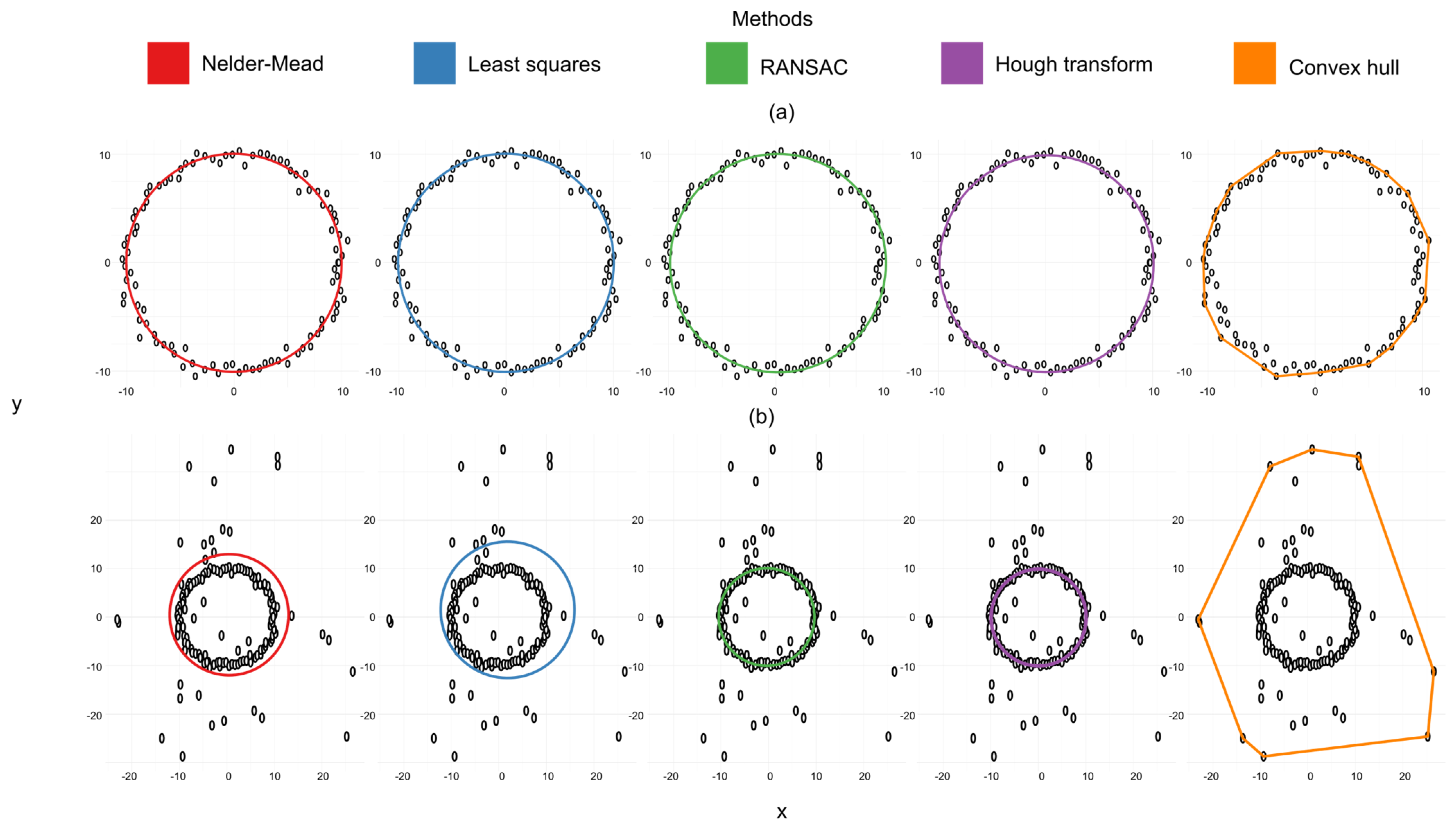
The response of the different algorithms to stem circumference estimation varies significantly, reflecting their distinct approaches to handling geometric data. In the graphical representation (Figure 6), Nelder–Mead and least squares closely follow the shape of the stem, providing consistent diameter estimates without significant deviation from the geometric center. Hough transform behaves similarly but tends to slightly underestimate in certain areas. In contrast, convex hull consistently overestimates the diameter, especially in the lower left part of the graph, indicating it may be less suited for capturing precise tree contours.

As for RANSAC, it produces a smaller circumference, primarily fitting areas with higher point density, such as the left and right sides of the graph. Unlike the other methods that tend to capture the whole stem, RANSAC prioritizes denser zones and omits more distant points, leading to underestimations of the diameter in various sections. Together, these algorithms offer different approaches to fitting the circumference, with methods like Nelder–Mead and least squares being more accurate, while others like convex hull and RANSAC show greater variability in their estimates. Additional examples of circumferences and the respective responses of the algorithms can be found in Appendix C, in Figure A3 and Figure A4.

Table 5. Coefficient of determination values for five fitting methods.

Methods	Austria	Guyana	Indonesia	México	Perú	Switzerland
a 1	0.82	0.66	0.75	0.98	0.72	0.87
b	0.79	0.61	0.79	0.98	0.82	0.89
c	0.82	0.54	0.81	0.98	0.74	0.83
d	0.80	0.66	0.76	0.98	0.70	0.89
e	0.55	0.55	0.79	0.95	0.83	0.74

¹ a = Nelder–Mead, b = Least squares, c = RANSAC, d = Hough transform, e = Convex hull.

presents the coefficient of determination values for the six regions, obtained using five fitting methods. In general, the methods show a good fit with R² values close to 1.0.

The Nelder–Mead method exhibits the highest value for Mexico (0.982), followed by Switzerland (0.873) and Austria (0.823). Least squares achieve coefficients close to 1.0 in Mexico (0.982) and Switzerland (0.886), while the convex hull method has the lowest value for Austria (0.552), highlighting a poor fitting capability in this region.

The bubble chart in Figure 7 provides a clear visualization of the different R² values among the methods in each country. In this chart, the size of each bubble is proportional to the R² value, meaning that larger bubbles indicate a higher R² and therefore a better fit. This design allows for a direct comparison of fit values both between algorithms and across regions. For example, an excellent fit is observed in Mexico and Switzerland, where larger bubbles are seen, while lower accuracy is indicated by smaller bubbles in countries like Guyana and Austria. The scatter plot images can be found in Appendix D, Figure A5 and Figure A6.

RMSE and mean absolute relative error are common error analysis metrics used to evaluate the accuracy and consistency of different measurement or fitting methods in studies such as tree diameter estimation.

RMSE measures the average deviation between observed values and estimates in absolute terms. This calculation is based on squaring the differences of each pair of values, which penalizes larger errors and captures overall variability more effectively. A low RMSE indicates that the method produces estimates close to the observed values on average, suggesting high reliability and low error variability. Conversely, a high RMSE reflects greater dispersion in errors, implying that the estimates deviate significantly from the actual values.

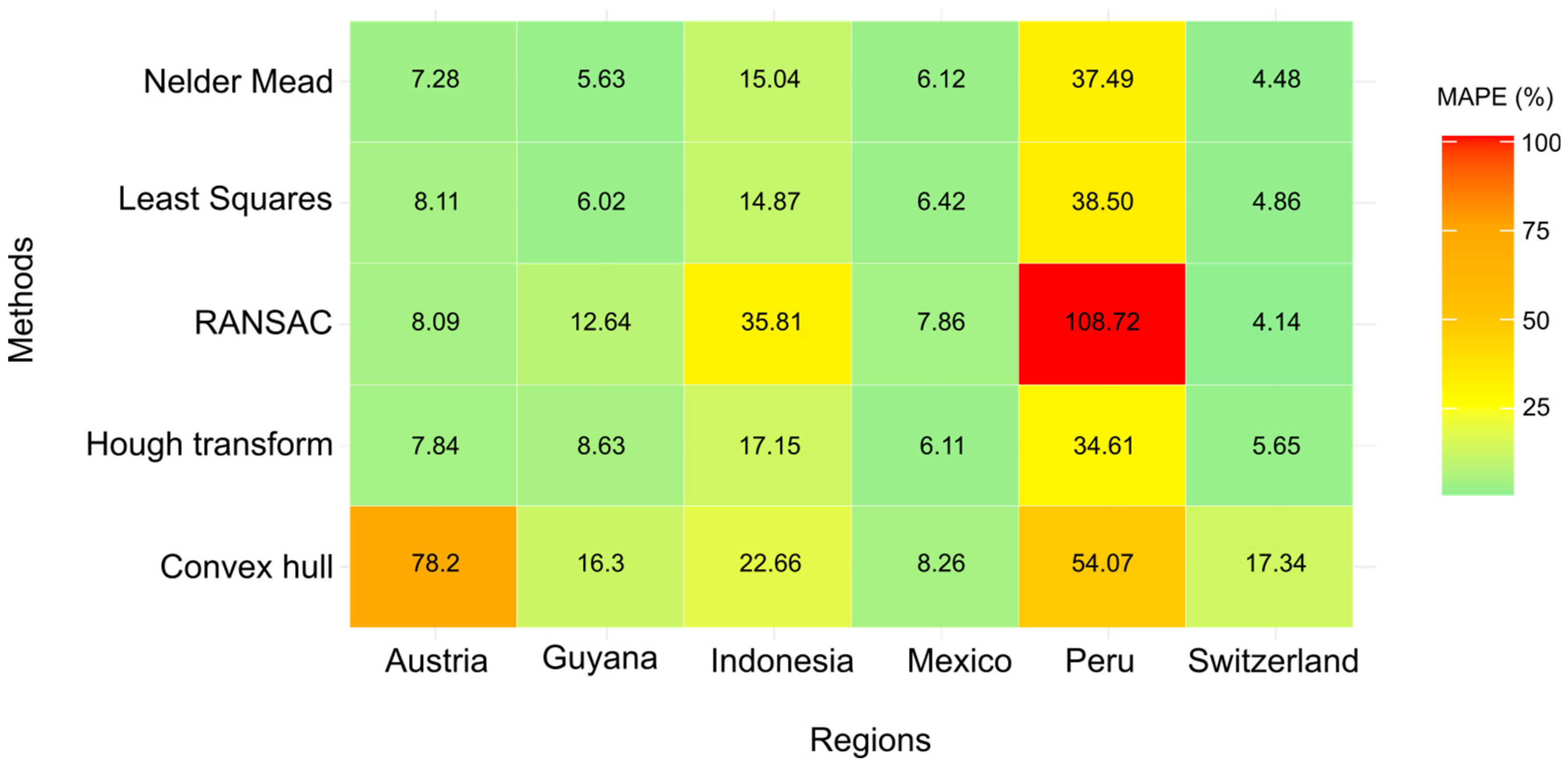
On the other hand, MAPE calculates the average error in relative terms, expressing each error as a percentage of the observed value. This allows the method’s accuracy to be evaluated in relation to the size of the observed values, making it especially useful for studies with varying magnitudes. As a percentage metric, MAPE facilitates the comparison of model or method performance across different scales or units of measurement, enabling consistent assessment regardless of the data scale.

Thus, a method with low RMSE and MAPE values is generally considered superior, as it reflects both low error variability and high relative accuracy. This combination makes the method more adaptable to different contexts and provides reliable and comparable estimates in scientific studies.

RMSE and MAPE values for the six datasets are summarized in

Table 6. Summary of RMSE and mean relative error for the fitting methods.

	Austria		Guyana		Indonesia		Mexico		Peru		Switzerland
Methods	RMSE (cm)	MAPE (%)	RMSE (cm)	MAPE (%)	RMSE (cm)	MAPE (%)	RMSE (cm)	MAPE (%)	RMSE (cm)	MAPE (%)	RMSE (cm)	MAPE (%)
a 1	4.66	7.28	9.11	5.63	22.98	15.04	1.59	6.12	50.55	37.49	6.02	4.48
b	5.39	8.11	10.02	6.02	21.64	14.87	1.67	6.42	48.21	38.50	5.93	4.86
c	4.00	8.09	11.48	12.64	58.26	35.81	1.80	7.86	162.86	108.72	6.12	4.14
d	4.49	7.84	10.27	8.63	21.80	17.15	1.71	6.11	48.60	34.61	5.50	5.65
e	31.67	78.2	16.89	16.3	26.46	22.66	2.81	8.26	67.89	54.07	13.45	17.34

¹ a = Nelder–Mead, b = Least squares, c = RANSAC, d = Hough transform, e = Convex hull.

, based on five fitting methods.

For Austria, the Nelder–Mead and RANSAC methods yielded the lowest RMSE values, at 4.66 cm and 4 cm, respectively. In contrast, the convex hull method exhibited a significantly poorer performance, with an RMSE of 31.67 cm. Regarding MAPE, the lowest percentages were achieved by the Nelder–Mead (7.28%) and Hough transform (7.84%) methods, while convex hull reached a notably high 78.2%, marking the worst outcome for this region.

In Guyana, Nelder–Mead and least squares emerged as the most precise methods, with RMSE values of 9.11 cm and 10.02 cm, respectively. Conversely, the convex hull method again showed the highest error, with an RMSE of 16.89 cm. MAPE results followed a similar trend, where Nelder–Mead and least squares recorded the lowest percentages at 5.63% and 6.02%, while convex hull registered the highest at 16.3%.

Indonesia demonstrated a broader variation among methods. Nelder–Mead and least squares maintained relatively low RMSEs, at 22.98 cm and 21.64 cm, respectively, whereas RANSAC underperformed significantly, with an RMSE of 58.26 cm. This pattern was consistent in the MAPE results, where RANSAC reached 35.81%, in contrast to the more moderate values of 15.04% for Nelder–Mead and 14.87% for least squares.

Mexico exhibited the lowest errors overall. The Nelder–Mead method stood out as the most accurate, with an RMSE of 1.59 cm and a MAPE of 6.12%. Although the convex hull method displayed a slightly higher RMSE (2.81 cm), it remained relatively low compared to the other countries.

In Peru, results showed considerable variability. The Nelder–Mead, least squares, and Hough transform methods achieved RMSE values close to 50 cm. However, RANSAC performed notably poorly, with an RMSE of 162.86 cm and an exceptionally high MAPE of 108.72%. Convex hull also showed suboptimal performance, with an RMSE of 67.89 cm and a MAPE of 54.07%.

For Switzerland, the performance of the Nelder–Mead, least squares, RANSAC, and Hough transform methods was more balanced, with RMSE values around 6 cm. Nevertheless, convex hull again displayed the worst performance, with an RMSE of 13.45 cm and a MAPE of 17.34%. In contrast, least squares recorded the best relative performance, with a MAPE of 4.48%.

The heat maps of RMSE and MAPE (Figure 8 and Figure 9) illustrate the differences between methods and regions. In these maps, green indicates low error, while red represents very high error. The convex hull method consistently produced the highest errors, both in absolute and relative terms, while the Nelder–Mead, least squares, and Hough transform methods provided more stable and reliable results, particularly in countries such as Mexico and Switzerland, where errors remained minimal.

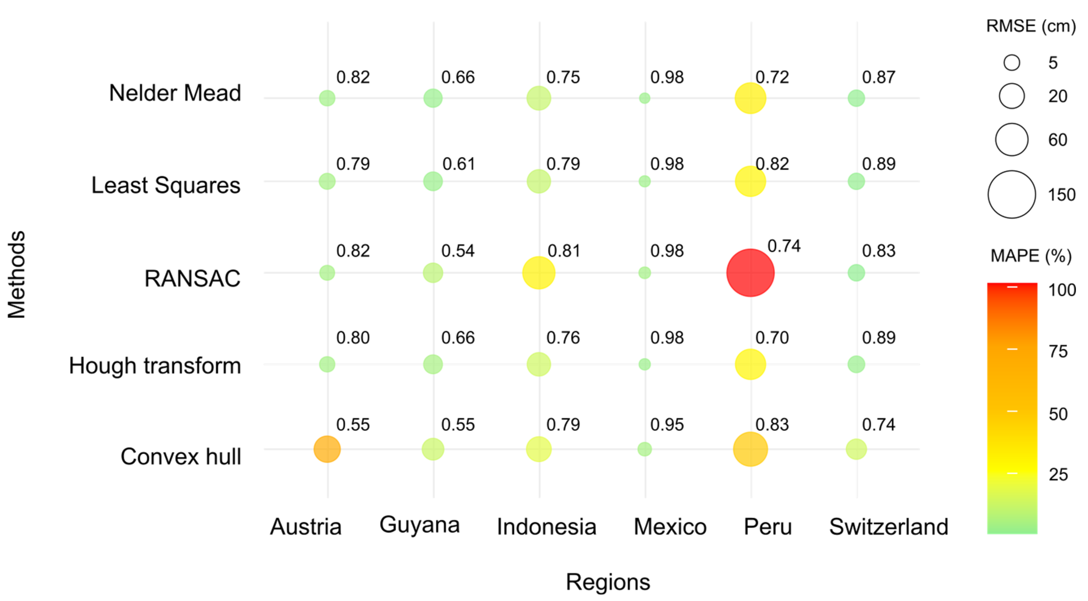
Figure 10 is a combination of a bubble chart and a heat map that summarizes all the information related to RMSE, MAPE, and R². In this chart, RMSE is represented by the size of the bubbles, MAPE defines the color gradient, and R² is shown as the subscript within each bubble. This design enables direct comparison between methods and regions. The ideal values are represented by small green circles with R² values close to 1, as seen in the case of Mexico.

Finally, the results of the bootstrapping are included in Appendix E,

Table A2. Confidence intervals from bootstrapping for Nelder–Mead, least squares, and RANSAC.

		Confidence Interval 95%
Methods		Austria	Guyana	Indonesia	Mexico	Peru	Switzerland
a I	Mean DHB (cm) LB II	37.37	68.01	48.44	18.01	90.73	46.5
	Mean DHB (cm) UB III	41.65	85.42	92.54	24.48	165.56	53.93
	R2 LB	0.73	0.35	0.65	0.95	0.47	0.78
	R2 UB	0.9	0.99	0.98	0.99	0.99	0.98
	RMSE (cm) LB	3.06	1.31	3.85	1.16	22.49	2.1
	RMSE (cm) UB	5.99	15.61	38.77	2.02	78.21	9.26
	MAPE (%) LB	5.43	1.62	4.19	4.82	17.86	2.45
	MAPE (%) UB	9.37	12.89	31.38	7.45	63.58	7.35
b	Mean DHB (cm) LB	37.75	67.58	48.64	17.5	92.6	46.05
	Mean DHB (cm) UB	42.41	86.9	90.37	24.54	160.92	53.79
	R2 LB	0.69	0.25	0.68	0.95	0.64	0.84
	R2 UB	0.88	0.99	0.98	0.99	0.99	0.96
	RMSE (cm) LB	3.65	1.29	4.05	1.23	25.16	2.53
	RMSE (cm) UB	6.91	17.21	36.21	2.13	69.55	9.07
	MAPE (%) LB	6.05	1.62	4.67	4.95	20.24	2.94
	MAPE (%) UB	10.35	14.07	31.18	7.9	60.18	7.29
c	Mean DHB (cm) LB	34.89	59.02	47.99	17.11	114.24	44.6
	Mean DHB (cm) UB	38.7	77.87	130.77	23.91	300.9	51.92
	R2 LB	0.73	0.16	0.58	0.95	0.49	0.77
	R2 UB	0.88	0.87	0.95	0.99	0.98	0.98
	RMSE (cm) LB	3.33	7.42	6.79	1.48	67.4	1.8
	RMSE (cm) UB	4.62	14.48	92.75	2.08	239.9	10.2
	MAPE (%) LB	6.58	6.59	9.1	6.16	42.95	2.56
	MAPE (%) UB	9.49	18.96	72.42	9.5	183.29	6.69

^I a = Nelder–Mead, b = Least squares, c = RANSAC, ^II LB = Lower bound, ^III UP = Upper bound.

and

Table A3. Confidence intervals from bootstrapping for Hough transform and convex hull.

		Confidence Interval 95%
Methods		Austria	Guyana	Indonesia	Mexico	Peru	Switzerland
d I	Mean DHB (cm) LB II	35.83	70.04	46.46	18.24	87.77	46.65
	Mean DHB (cm) UB III	40.23	88.16	87.83	24.84	160.73	54.09
	R2 LB	0.69	0.35	0.55	0.95	0.43	0.79
	R2 UB	0.89	0.96	0.95	0.99	0.99	0.97
	RMSE (cm) LB	3.15	2.84	6.14	1.28	19.15	2.52
	RMSE (cm) UB	6	15.89	35.75	2.13	75.64	7.96
	MAPE (%) LB	6.22	3.22	7.28	4.51	15.24	3.84
	MAPE (%) UB	9.62	15.63	31.27	7.93	58.73	7.96
e	Mean DHB (cm) LB	63.11	75.8	52.7	17.88	100.31	51.06
	Mean DHB (cm) UB	70.88	97.16	99.14	23.76	184.72	60.91
	R2 LB	0.43	0.25	0.66	0.85	0.66	0.62
	R2 UB	0.69	0.99	0.98	0.98	0.97	0.83
	RMSE (cm) LB	28.23	7.25	6.16	1.75	35.94	9.52
	RMSE (cm) UB	35.71	27.02	43.12	4.01	92.96	16.95
	MAPE (%) LB	72.26	9.59	11.08	6.19	29.65	13.07
	MAPE (%) UB	85.51	27.9	39.75	10.62	79.01	21.9

^I d = Hough transform, e = Convex hull, ^II LB = Lower bound, ^III UP = Upper bound.

. For each metric (DBH, R², RMSE, and MAPE), the bootstrap method was applied, generating a distribution of 1,000 samples with replacement, which allowed for the construction of 95% confidence intervals. These intervals provide a measure of the stability and variability of the results under conditions similar to those observed in the field. For example, the confidence interval for RMSE in the RANSAC method (Mexico) ranged between 1.48 and 2.08; this range could be expected with 95% confidence in a large-scale study in a forest with similar environmental characteristics. In this way, the confidence intervals strengthen the comparability between methods and provide an estimate of the inherent uncertainty in the data.

Nelder–Mead, in Austria, shows narrow intervals for the mean DBH (37.37–41.65 cm) and RMSE (3.06–5.99 cm), with R² values between 0.73 and 0.9. Convex hull, however, exhibits the widest ranges, with RMSE values between 28.23 and 35.71 cm and R² spanning from 0.43 to 0.69. The Hough transform method shows moderate RMSE intervals (3.15–6.00 cm), with R² ranging between 0.69 and 0.89.

In Guyana, Nelder–Mead and least squares maintain RMSE values between 1.31 cm (lower bound) and 17.21 cm (upper bound), though the R² range is broader. RANSAC and convex hull display wider RMSE intervals, reaching up to 27.02 cm. The Hough transform reports an RMSE between 2.84 and 15.89 cm, with R² values ranging from 0.35 to 0.96.

For Indonesia, Nelder–Mead and least squares exhibit moderate intervals, though the R² ranges are relatively broad. RANSAC and convex hull show greater dispersion, particularly in RMSE, with RANSAC reaching values as high as 92.75 cm. The Hough transform method demonstrates RMSE values between 6.14 and 35.75 cm, with R² ranging from 0.55 to 0.95.

Regarding Mexico, the methods present narrow intervals for both the mean DBH and RMSE, with R² values close to 1. Nelder–Mead reports an RMSE between 1.16 and 2.02 cm, while convex hull’s RMSE ranges from 1.75 to 4.01 cm. The Hough transform displays RMSE values between 1.28 and 2.13 cm.

The results for Peru reflect greater overall dispersion. RANSAC exhibits the highest RMSE, with intervals spanning from 67.4 to 239.9 cm, while convex hull also displays high variability. Nelder–Mead and least squares show considerable variation in both R² and RMSE. The Hough transform registers RMSE values between 19.15 and 75.64 cm, with R² values ranging from 0.43 to 0.99.

Ultimately, in Switzerland, Nelder–Mead and least squares stand out with narrow intervals for both the mean DBH and RMSE. RANSAC maintains a relatively low RMSE, while convex hull shows an RMSE range between 9.52 and 16.95 cm. The Hough transform method presents an RMSE between 2.52 and 7.96 cm, with R² values ranging from 0.79 to 0.97.

4. Discussion

4.1. Behavior and Comparison of Algorithms on Simulated Data

In this study, circle fitting methods were evaluated under various simulated scenarios, including data with distributed outliers, clustered values in a specific region, circular arcs, and additive noise in the points forming the circle boundaries. The results indicated that the methods can fit circles in datasets exhibiting some degree of variance, making it feasible to use any of the tested methods. However, in the case of distributed outliers, non-robust methods such as Nelder–Mead, least squares, and convex hull showed high sensitivity to noise, resulting in a significant increase in the mean squared error and greater dispersion in the estimates of the circle’s center and radius. This behavior aligns with the findings of Nurunnabi et al. [38], who highlighted the vulnerability of least squares-based methods when dealing with contaminated data.

In the presence of unwanted data clustering, non-robust methods began to exhibit unstable behavior, with a substantial increase in both the variance and bias of the estimates. This reflects the observations made by Nurunnabi et al. [38], who found that algebraic and geometric methods, such as Pratt and Taubin, also experienced significant bias when exposed to such outliers, leading to the overestimation of radii and incorrect positioning of the circle’s center. In our simulations, the MSE for Nelder–Mead and least squares in the presence of 20% clustered outliers reached critical values, while convex hull performed even more erratically.

Consistent with the work authored by Nurunnabi et al. [38], our results showed that robust methods, such as RANSAC and Hough transform, had a higher tolerance to noise compared to non-robust methods. However, in our simulations with clustering and incomplete circles, the RANSAC method displayed limitations, corroborating Nurunnabi et al.‘s findings on its sensitivity to thresholded errors, where undetected outliers compromise the fitting accuracy. In contrast, the Hough transform maintained acceptable performance even in scenarios with incomplete data.

The results of our study demonstrate that, at least under simulated conditions, circle-fitting algorithms exhibit predictable behavior based on their robustness to outliers. Non-robust methods, such as Nelder–Mead and least squares, proved to be more sensitive to noise and clustered outliers, leading to a significant increase in error and dispersion in the estimates. Conversely, robust methods like RANSAC and Hough transform showed greater resilience to disturbances, maintaining adequate performance even in contaminated data scenarios. These findings corroborate previous literature and suggest that, under controlled conditions, the algorithms generally behave according to their theoretical principles, providing a clear expectation of their performance in real-world situations with similar characteristics.

4.2. Comparison of Algorithms on TLS Data Across Regions and Devices

4.2.1. Multiscan Approach and Devices

This section compares different scanning devices used in tree diameter estimation studies, focusing on their efficiency and accuracy across various forest types.

The implementation of multiple scans is essential in TLS use, as point cloud quality can be compromised by occlusions and other environmental factors. Abegg et al. [39] emphasized that the strategic placement of the scanner and the distribution of trees within a plot are critical factors influencing DBH measurement accuracy. Similarly, Liang et al. [40], in an international comparative analysis of TLS approaches, demonstrated that multiple scans significantly improve data completeness and DBH estimation accuracy, especially in dense and complex forest environments. These findings are consistent with those of Liu et al. [11], who concluded that scanning from multiple positions provides a more detailed representation of the trunk, reducing interference from understory vegetation and minimizing noise in the data.

In Mexico, we implemented four scans per tree from different directions to mitigate occlusion effects and maximize trunk coverage. The experimental plot has a tree density of 960 trees per hectare, predominantly in temperate forest settings. This approach yielded high-quality data, generating nearly complete 3D models of the trunks and significantly reducing noise. Our results confirm that the multiscan strategy improves DBH estimation accuracy, particularly in densely wooded areas, consistent with previous studies. A comparable study, both in terms of forest type and number of scans, is “Individual Tree Volume Estimation with Terrestrial Laser Scanning: Evaluating Reconstructive and Allometric Approaches,” [21] which applied three scans in the study area.

In tropical forests, where tree species and ecosystem structure differ significantly, multiple scans are essential. This is demonstrated in the study “Estimation of Above-Ground Biomass of Large Tropical Trees with Terrestrial LiDAR,” [22] where up to 13 scans per tree were conducted to adequately capture the irregular geometry of the trunks.

When comparing scanning devices such as the GeoSLAM ZEB Horizon (GeoSLAM Ltd., Nottingham, UK), RIEGL VZ-400 (RIEGL Laser Measurement Systems GmbH, Horn, Austria), FARO Focus M70 (FARO, Lake Mary, FL, USA) and Leica BLK360 (Leica Geosystems, Heerbrugg, Switzerland), each presents unique characteristics depending on the capture methodology and environmental requirements. The ZEB Horizon (GeoSLAM Ltd., Nottingham, UK) is a mobile scanner that uses SLAM technology, enabling continuous data capture without the need for multiple scans from fixed positions. This characteristic makes it highly efficient in large or difficult-to-access areas where rapid data collection is essential. However, its maximum range is limited to 100 m, with a noise precision of ±30 mm. This device is most effective in closed spaces with high reflectivity, but its accuracy and detail are compromised at greater distances or in low-reflectivity environments. Additionally, its scan rate of 300,000 points per second provides a moderate point density; however, compared to fixed scanners like the RIEGL VZ-400 (RIEGL Laser Measurement Systems GmbH, Horn, Austria) or the FARO Focus M70 (FARO, Lake Mary, FL, USA), the GeoSLAM ZEB Horizon (GeoSLAM Ltd., Nottingham, UK) produces higher levels of noise. While SLAM technology increases the scanner’s flexibility for mobile scanning, it may also introduce cumulative errors over long trajectories if loop closures are not applied correctly [23].

The RIEGL VZ-400 (RIEGL Laser Measurement Systems GmbH, Horn, Austria), in contrast, is a high-precision terrestrial scanner with a maximum range of up to 600 m for high-reflectivity targets and sub-millimeter accuracy of up to 5 mm. This capability, along with the option to operate in long-range or high-speed modes, makes it suitable for applications requiring high precision, especially in topographic and georeferencing projects. With an effective measurement rate of 122,000 points per second and detailed angular control, the RIEGL VZ-400 (RIEGL Laser Measurement Systems GmbH, Horn, Austria) can generate high-density point clouds with low noise. Unlike the GeoSLAM ZEB Horizon (GeoSLAM Ltd., Nottingham, UK), the RIEGL VZ-400 (RIEGL Laser Measurement Systems GmbH, Horn, Austria) requires strict stabilization and field control, benefiting from strategically placed tie points around the scanner to optimize spatial accuracy. Its ability to detect multiple targets in a single laser pulse further supports its application in complex terrain and large-scale geospatial studies, where data stability and quality are critical [24].

The FARO Focus M70 (FARO, Lake Mary, FL, USA), although with a more limited range than the RIEGL VZ-400 (RIEGL Laser Measurement Systems GmbH, Horn, Austria), provides a capture rate of up to 976,000 points per second in advanced models and achieves high accuracy through phase-shift technology. Its range varies by model, with the FARO Focus M70 (FARO, Lake Mary, FL, USA) capable of reaching up to 70 m, making it a suitable option for smaller or less complex areas, balancing accuracy with data capture speed. Its adjustable resolution and scanning quality offer flexibility for short- and medium-range projects requiring detailed visual accuracy. In contrast to the GeoSLAM ZEB Horizon (GeoSLAM Ltd., Nottingham, UK), whose mobility compensates in part for its lower precision, the FARO Focus M70 (FARO, Lake Mary, FL, USA) is ideal for static applications in moderately sized areas. Its dual-axis compensator ensures effective automatic leveling on flat surfaces, and although it does not match the range of the RIEGL VZ-400 (RIEGL Laser Measurement Systems GmbH, Horn, Austria), it proves useful in architectural and interior studies where color scanning and detailed object documentation are essential [25].

The Leica BLK360 (Leica Geosystems, Heerbrugg, Switzerland), on the other hand, is an efficient option for moderate-precision surveys with a range of up to 60 m. With a precision of 6 mm at 10 m, it is suitable for controlled environments requiring high levels of detail without the need for sub-millimeter precision. The device’s capture rate of 360,000 points per second situates it between the FARO Focus M70 (FARO, Lake Mary, FL, USA) and the GeoSLAM ZEB Horizon (GeoSLAM Ltd., Nottingham, UK) in terms of speed. However, its HDR spherical imaging capability and ability to generate high-resolution scans at varying point densities allow its use in documentation and conservation projects. Despite its limited range relative to the RIEGL VZ-400 (RIEGL Laser Measurement Systems GmbH, Horn, Austria), the Leica BLK360 (Leica Geosystems, Heerbrugg, Switzerland) combines portability and visual accuracy, favoring its application in architectural studies and indoor spaces. Nonetheless, it is not as suitable for large-scale studies due to range limitations and a need for higher precision [26].

It is important to emphasize that point density is a key factor in forestry studies, as it enables a detailed representation of the trunk and improves DBH estimation accuracy, particularly in dense areas where understory vegetation can interfere with measurements. When analyzing these devices, the study by Abegg et al. [41] highlights that point cloud accuracy in forest environments is strongly influenced by laser beam diameter and scanning approach. Devices like the RIEGL VZ-1000 (RIEGL Laser Measurement Systems GmbH, Horn, Austria), with multi-signal capabilities, demonstrated effectiveness in detecting small objects and enhancing point cloud quality in dense forests, although this configuration may introduce some noise. Conversely, the compact Leica BLK360 (Leica Geosystems, Heerbrugg, Switzerland) has limitations in range (60 m) and resolution, making it less suitable for large-scale studies or applications requiring high precision.

The FARO Focus M70 (FARO, Lake Mary, FL, USA), used in Mexico, with its limited range of 70 m, balances precision with speed, making it applicable in smaller or simpler environments. However, its performance may be limited in larger or more structurally complex areas compared to devices with a longer range. As Abegg et al. [41] noted, devices with larger beam diameters tend to generate mixed-pixel effects and reduced precision for smaller objects, which could impact data quality in denser forest environments.

In summary, the choice of device depends on the study environment and required precision level, with the GeoSLAM ZEB Horizon (GeoSLAM Ltd., Nottingham, UK) being more suitable for large, hard-to-reach areas, while devices like the FARO Focus M70 (FARO, Lake Mary, FL, USA) offer higher precision in more controlled settings. For studies in complex environments with dense vegetation, factors such as point density and laser beam accuracy must be carefully considered.

4.2.2. DBH Estimation

The accuracy of TLS measurements in complex forest environments is influenced by environmental and structural factors, such as vegetation density, canopy complexity, topography, and meteorological conditions. Dense vegetation and branch arrangement introduce noise that complicates precise trunk detection [20,28], while irregular topography can distort data, especially on sloped terrain [20,42]. Additionally, factors like scanner type and position, as well as weather conditions (e.g., wind), impact data quality [21]. Dense understory vegetation further introduces noise, complicating trunk segmentation and affecting measurements of individual tree characteristics [20].

In Austria’s mixed forests, comprising both broadleaf and coniferous species, Nelder–Mead (R² = 0.82, RMSE = 4.66 cm, MAPE = 7.28%) proved to be the most effective, with RMSE within the acceptable range and MAPE indicating high relative accuracy. RANSAC also achieved an R² of 0.82 but with a higher MAPE of 8.09%, indicating slightly lower relative accuracy. The convex hull method showed poorer performance (RMSE of 31.67 cm), impacted by the dense vegetation introducing occlusion in the data [20,28].

Similarly, in Guyana’s peat swamp forests (516 stems ha⁻¹), Nelder–Mead once again yielded the best results (R² = 0.66, RMSE = 9.11 cm, MAPE = 5.63%), which, despite being in the regular RMSE range, maintained a low MAPE, suggesting it handles relative accuracy well in this region. In contrast, RANSAC performed the worst in Guyana (R² = 0.54, RMSE = 11.48 cm, MAPE = 12.64%), with a high RMSE indicating poor absolute accuracy. Wu et al. [42] reported similar findings, where RANSAC showed a high absolute error of 16.90 cm in large tropical trees, likely due to the method’s difficulty in adapting to the complex structures in dense forests. The high density of understory vegetation in tropical forests, combined with irregular trunk geometries, seems to interfere with RANSAC’s fitting accuracy, as dense foliage increases noise in the point cloud, reducing the method’s ability to accurately capture trunk shape. The convex hull method had high errors (RMSE of 16.89 cm) due to interference from dense vegetation during scanning [21,22].

Indonesia’s tropical moist forest (stem density of 1314 stems ha⁻¹) presented a high variability in algorithm performance, where Nelder–Mead was effective (R² = 0.81, RMSE = 22.98 cm, MAPE = 15.04%) but still fell into the poor RMSE range. However, RANSAC showed particularly poor performance in this region (RMSE = 58.26 cm, MAPE = 35.81%), which is attributed to occlusions created by large, irregularly shaped trees that affect the algorithm’s accuracy [42] and supporting the analysis by Srinivasan et al. [43] that RANSAC may struggle in environments with complex geometries. Lee and Lee [17] found that RANSAC performed better under optimized conditions, achieving an RMSE as low as 0.97 cm, highlighting that adjustments can mitigate some errors. The Hough transform also showed subpar performance (RMSE = 21.80 cm, MAPE = 17.15%), aligning with Wu et al. [42], who noted that the Hough transform has limited accuracy in complex structures with large errors in tree diameter estimation. In Indonesia, the combination of uneven topography and dense vegetation may have contributed to the higher errors observed in RANSAC and the Hough transform, as these environmental factors introduce additional challenges for algorithms that rely on regular geometric assumptions.

Mexico, our primary region of interest, demonstrated the impact of data quality on algorithm performance. Here, Nelder–Mead proved to be the best method (R² = 0.98, RMSE = 1.59 cm, MAPE = 6.12%), closely followed by least squares (R² = 0.98, RMSE = 1.67 cm, MAPE = 6.42%), both achieving RMSE values in the acceptable range. These results indicate high accuracy in both absolute and relative terms; this suggests that lower vegetation density and simpler structural complexity facilitate more precise data capture [44]. RANSAC also performed adequately (R² = 0.98, RMSE = 1.80 cm, MAPE = 7.86%), highlighting the importance of high-quality data in achieving precise DBH measurements.

A key feature of the trees in the Mexican plot studied is that a large proportion of the species belong to the Pinus family, with trunks that tend to be more regular and uniform compared to species like Quercus or tropical trees. This morphological consistency allows fitting algorithms like Nelder–Mead and least squares to perform optimally. Conversely, species with irregular geometries pose greater challenges, potentially impacting DBH accuracy, especially in regions with higher trunk structural variability.

In Peru, lowland tropical forests with high vegetation density exhibited a wide range of errors. Convex hull emerged as the most effective method (R² = 0.83, RMSE = 48.60 cm, MAPE = 34.61%), despite its RMSE and MAPE falling into the poor range, outperforming traditional methods like least squares in this region. However, RANSAC performed very poorly in Peru (R² = 0.74, RMSE = 162.86 cm, MAPE = 108.72%), consistent with the behavior observed in large tropical trees by Wu et al. [42]. This reflects RANSAC’s limitations when dealing with irregular, large-scale geometries in tropical environments. indicating a need for more robust algorithms to handle irregular structures and high-density environments [22].

In Switzerland, least squares provided the most accurate estimates (R² = 0.89, RMSE = 5.93 cm, MAPE = 4.86%), followed by Nelder–Mead (R² = 0.87, RMSE = 6.02 cm, MAPE = 4.48%), both within the acceptable RMSE and MAPE ranges. In contrast, the Hough transform showed inferior performance (R² = 0.74, RMSE = 6.50 cm, MAPE = 5.65%), consistent with its reduced reliability in simpler tree structures. However, the convex hull method was again the least accurate (RMSE of 13.45 cm), underscoring its inefficacy in areas with dense vegetation and steep slopes [21].

These findings are consistent with those of You et al. [29], who observed that 3D methods, such as cylindrical fitting, tend to achieve higher accuracy compared to 2D methods, such as circular fitting.

Results confirm that the effectiveness of fitting methods varies based on environmental characteristics: simpler algorithms like Nelder–Mead and least squares demonstrate consistent accuracy in regions with lower structural complexity, such as Mexico and Switzerland, while more complex geometries, like those in Peru, present challenges for traditional methods. Balancing precision with algorithmic complexity is crucial for accurate DBH estimation. Although Nelder-Mead and least squares perform robustly with minimal computational requirements, making them suitable for simpler environments, more computationally intensive methods, such as the Hough transform, may perform better in noisier conditions but face scalability issues. RANSAC, while effective with outliers and complex geometries, shows limitations in regions with high variability, emphasizing the need for algorithms that align not only with the desired accuracy but also with the complexity and scalability demands of each specific forest environment.

4.2.3. Bootstrapping

The analysis of the methods reveals clear trends in their performance across different countries. In general, Nelder–Mead and least squares stand out as the most reliable, while convex hull consistently shows the worst performance. This trend is reflected in both the goodness of fit and absolute and relative errors, though with variations between countries.

In the case of Mexico, both Nelder–Mead and least squares show excellent fit, with R² close to 0.99 and low RMSE values (1.16 to 2.13 cm) and MAPE values (4.82 to 7.90%) demonstrating their precision and consistency. RANSAC, although competitive, shows slightly greater error dispersion. However, convex hull stands out for its inferior performance, with broader RMSE values (1.75 to 4.01 cm) and higher MAPE values (6.19 to 10.62%), making it the least reliable. Here, Nelder–Mead emerges as the best option for accurate predictions.

A similar pattern is observed in Austria, where Nelder–Mead and RANSAC strike a balance between good fit (R² between 0.73 and 0.90) and controlled errors (RMSE between 3.06 and 4.62 cm). While reliable, least squares shows greater error dispersion, whereas convex hull once again shows poor performance, with significantly higher RMSE values (28.23 to 35.71 cm) and high MAPE values (72.26 to 85.51%).

When examining performance in Guyana, there is greater error variability, especially with Nelder–Mead and least squares, which show wide ranges in R² and RMSE, suggesting variability in the errors. Despite this variability, both methods outperform RANSAC and convex hull, which show significantly higher errors and lower reliability. It is possible that the number of trees and values that could be considered outliers introduce greater uncertainty in the reliability of the methods. This may be due to the greater variability in tree structures in the tropical forests of Guyana, which introduces more uncertainty in the estimates.

In Peru, all methods show high uncertainty, with wide error ranges in RMSE and MAPE. Although Nelder–Mead and least squares achieve the best fit, their errors are much more variable, reaching RMSE values as high as 78.21 cm. RANSAC and convex hull fall to the lower end of performance, with very high error levels. The high uncertainty in these methods limits their reliability.

Finally, in Switzerland, Nelder–Mead and least squares again offer solid performance, with consistent fits (R² between 0.84 and 0.96) and well-controlled errors. Although RANSAC shows greater error variability, it remains competitive. However, convex hull again proves to be the worst method, with elevated errors and less precise predictions. Therefore, Nelder–Mead remains the best option in this country, providing more precise and consistent predictions.

Despite the promising results presented in this study, it is important to acknowledge several limitations when interpreting the findings. Firstly, while algebraic algorithms, such as Nelder–Mead and least squares, and robust methods, like RANSAC and Hough transform, demonstrated good performance in simulated environments, their application in real forest settings may be influenced by factors not fully accounted for in this study. Species-specific growth patterns, understory interference, and varying topographic conditions introduce additional challenges that can affect both algebraic and robust methods. While algebraic algorithms are more efficient in controlled environments and species with regular geometries, such as Pinus, they may experience reduced accuracy when dealing with more complex species or irregular geometries. On the other hand, robust algorithms, although less sensitive to outliers and noisy data, are not without limitations, particularly when facing highly irregular geometries like those found in tropical species. Additionally, inherent limitations of current TLS devices, such as limited range and sensitivity to occlusions, pose challenges for both types of algorithms, affecting the quality of the collected data.

Furthermore, in large-scale applications, the need for automated segmentation becomes critical. Efficient and accurate segmentation of point clouds is necessary to isolate individual trees or tree parts for processing by the fitting algorithms. This process can introduce additional computational complexity and potential inaccuracies, especially in dense or heterogeneous forest environments. The performance of both algebraic and robust methods may be impacted by the quality of the segmentation, making it a crucial step for large-scale forest assessments.

To overcome these limitations, it is essential to continue improving both algebraic and robust algorithms, as well as scanning technology, in order to adapt to the wide variety of conditions found in forest ecosystems.

4.2.4. Large-Scale Applications in Forest Management

The findings of this study highlight the potential of TLS for enhancing large-scale forest inventories by providing precise DBH measurements suitable across diverse forest configurations. The computational efficiency demonstrated by methods such as Nelder–Mead and least squares—particularly in datasets with simpler or more uniform tree structures—makes these methods advantageous for extensive monitoring. Their low processing times indicate they can be applied effectively in large-scale applications without significant computational strain.

However, in regions with dense vegetation or complex geometries, where methods like RANSAC and Hough transform show greater variability and require longer processing times, combining TLS with complementary technologies, such as airborne LiDAR, could improve coverage and allow for more accurate diameter and biomass estimations, especially in difficult-to-access areas.

Implementing TLS on a large scale offers substantial advantages for sustainable forest management, enabling continuous, detailed data collection that supports informed management and conservation decisions. Nevertheless, technical challenges remain, such as processing high-density data efficiently. Addressing these challenges through integrated technologies and optimized algorithms will be essential to ensure that TLS applications are both scalable and efficient across extensive forested landscapes.

4.2.5. Adaptation and Improvements for Tropical and Mixed Forests

DBH measurement in tropical and mixed forests is particularly challenging due to dense vegetation and irregular trunk structures. To enhance algorithm performance in these settings, the Nelder–Mead method could benefit from pre-processing via principal component analysis (PCA), which would help filter vegetation points and better isolate trunk sections. The least squares method, on the other hand, could be strengthened by incorporating bootstrapping techniques to generate average DBH estimates, thus reducing the impact of noise. Given its robustness against outliers, RANSAC could improve efficiency by implementing a Bayesian stopping criterion, optimizing processing time without compromising accuracy.

For computationally intensive algorithms such as the Hough transform, an adaptive sampling strategy, using Monte Carlo for point reduction, would decrease computational costs. Finally, the convex hull method, which tends to overestimate in irregular geometries, could be refined by probabilistic contour-smoothing models, such as Markov Random Fields, to better represent trunk shapes. These enhancements would allow the algorithms to adapt effectively to the complexities of tropical and mixed ecosystems, expanding their applicability across a broader range of forest conditions.

5. Conclusions

This study focused on evaluating the similarities and differences between various circle-fitting algorithms for estimating trunk diameter in forest environments, with a particular emphasis on temperate forests in Mexico.

The results revealed that Nelder–Mead (R² = 0.98, RMSE = 1.59 cm, MAPE = 6.12%) and least squares (R² = 0.98, RMSE = 1.67 cm, MAPE = 6.42%) stand out as the most reliable methods in the Mexican forests (Austria: R² = 0.82, RMSE = 4.66 cm, MAPE = 7.28%; Guyana: R² = 0.66, RMSE = 9.11 cm, MAPE = 5.63%; Indonesia: R² = 0.81, RMSE = 22.98 cm, MAPE = 15.04%; Peru: R² = 0.83, RMSE = 48.60 cm, MAPE = 34.61%; and Switzerland: R² = 0.89, RMSE = 5.93 cm, MAPE = 4.86%), providing good fits and low errors in R², RMSE, and MAPE. RANSAC (R² = 0.98, RMSE = 1.80 cm, MAPE = 7.86%), while competitive in some contexts, tends to show greater error variability. In contrast, convex hull (R² = 0.83, RMSE = 48.60 cm, MAPE = 34.61%) consistently demonstrates the worst performance, with wide error intervals and high uncertainty in predictions.

The good fit in the Mexican forests is largely due to the prevalence of Pinus species, whose trunk geometries tend to be more regular and symmetrical. These algorithms offer high accuracy in these environments due to their lower sensitivity to geometric variations, making them ideal for forest inventories and biomass estimations in temperate forest areas. While these results provide a general understanding of the expected behavior, certain reservations should be maintained in the analysis, as the precision and performance of the algorithms can depend significantly on the specific environmental conditions, data quality, and the number of trees included in the study, particularly in areas with more complex species and irregular trunk structures, such as tropical forests. This variability suggests that these methods may not be the most suitable for environments with high structural heterogeneity, highlighting the need for more robust approaches in such ecosystems. Additionally, the Hough transform (R² = 0.74, RMSE = 6.50 cm, MAPE = 5.65%), while versatile and applicable in a wide range of contexts, should be considered with caution due to its high computational cost, which may limit its practicality in large-scale applications or complex environments.

Data quality also played a crucial role in the performance of the algorithms. In the case of Mexico, the use of the FARO Focus M70 scanner, combined with a multiscan strategy, allowed for the generation of detailed and accurate 3D trunk models, significantly improving the estimation of DBH. To further ensure data precision, it is ideal to conduct scans under favorable weather conditions, avoiding rain and strong winds that may introduce noise and affect scan quality.

Lastly, the results emphasize the importance of the local context when selecting the appropriate algorithm. In regions like Mexico, where species with simple and regular geometries predominate, algebraic algorithms remain the most efficient option. In high density ecosystems with complex geometry, such as tropical forests, methods like RANSAC and convex hull exhibit significant limitations. The presence of dense vegetation and irregular trunk geometries introduces noise and occlusion in TLS data, affecting algorithm accuracy.

For broader forestry applications, it is recommended to enhance current algorithms by integrating preprocessing strategies, such as using PCA to filter noise or implementing adaptive sampling techniques. Furthermore, combining TLS with complementary technologies, such as aerial LiDAR, could optimize coverage in hard-to-access areas. Adapting these algorithms to improve accuracy across a wider range of ecosystems would be key to sustainable forest management and biomass estimation in complex environments.

Future studies should focus on applying TLS technologies in various Mexican ecosystems, including areas in Durango, such as the Pinus-Quercus forests in the Sierra Madre Occidental, as well as in other representative ecosystems of Mexico and the world, like arid zones, mangroves, or rainforests. Each of these environments presents unique challenges that require specific adaptations in algorithms and methodologies. Addressing these differences would not only improve the accuracy of biomass and DBH measurements in Mexico but also help create a reference framework adaptable to diverse ecosystems globally.

References

1. Yrttimaa, T.; Luoma, V.; Saarinen, N.; Kankare, V.; Junttila, S.; Holopainen, M.; Hyyppä, J.; Vastaranta, M. Structural Changes in Boreal Forests Can Be Quantified Using Terrestrial Laser Scanning. Remote Sens. 2020, 12, 2672. [Google Scholar] [CrossRef]
2. Chen, X.; Brockway, D.G. Height-Diameter Relationships in Longleaf Pine and Four Swamp Tree Species. J. Plant Stud. 2017, 6, 94. [Google Scholar] [CrossRef]
3. Xi, Z.; Chasmer, L.; Hopkinson, C. Delineating and Reconstructing 3D Forest Fuel Components and Volumes with Terrestrial Laser Scanning. Remote Sens. 2023, 15, 4778. [Google Scholar] [CrossRef]
4. Qin, S.; Nie, S.; Guan, Y.; Zhang, D.; Wang, C.; Zhang, X. Forest Emissions Reduction Assessment Using Airborne LiDAR for Biomass Estimation. Resour. Conserv. Recycl. 2022, 181, 106224. [Google Scholar] [CrossRef]
5. Vernimmen, R.; Hooijer, A.; Akmalia, R.; Fitranatanegara, N.; Mulyadi, D.; Yuherdha, A.; Andreas, H.; Page, S. Mapping Deep Peat Carbon Stock from a LiDAR Based DTM and Field Measurements, with Application to Eastern Sumatra. Carbon Balance Manag. 2020, 15, 4. [Google Scholar] [CrossRef]
6. Päivinen, R.; Nousiainen, M.; Korhonen, K.T. Accuracy of Certain Tree Measurements. Puutunnusten mittaamisen luotettavuus. Folia For. 1992, 787, 18. [Google Scholar]
7. Bu, G.; Wang, P. Adaptive Circle-Ellipse Fitting Method for Estimating Tree Diameter Based on Single Terrestrial Laser Scanning. J. Appl. Remote Sens. 2016, 10, 026040. [Google Scholar] [CrossRef]
8. Liu, G.; Wang, J.; Dong, P.; Chen, Y.; Liu, Z. Estimating Individual Tree Height and Diameter at Breast Height (DBH) from Terrestrial Laser Scanning (TLS) Data at Plot Level. Forests 2018, 9, 398. [Google Scholar] [CrossRef]
9. Montoya, O.; Icasio-Hernández, O.; Salas, J. TreeTool: A Tool for Detecting Trees and Estimating Their DBH Using Forest Point Clouds. SoftwareX 2021, 16, 100889. [Google Scholar] [CrossRef]
10. Islas-Gutiérrez, F.; Cruz-Juárez, E.; Buendía-Rodríguez, E.; Guerra-De La Cruz, V.; Pineda-Ojeda, T.; Flores-Ayala, E.; Carrillo-Anzures, F.; Acosta-Mireles, M. Ecuación alométrica para estimar biomasa aérea de árboles de Pinus hartwegii Lindl. A partir de datos lidar. Rev. Fitotec. Mex. 2024, 47, 70. [Google Scholar] [CrossRef]
11. Liu, C.; Xing, Y.; Duanmu, J.; Tian, X. Evaluating Different Methods for Estimating Diameter at Breast Height from Terrestrial Laser Scanning. Remote Sens. 2018, 10, 513. [Google Scholar] [CrossRef]
12. Wu, R.; Chen, Y.; Wang, C.; Li, J. Estimation of Forest Trees Diameter from Terrestrial Laser Scanning Point Clouds Based on a Circle Fitting Method. In Proceedings of the IGARSS 2018—2018 IEEE International Geoscience and Remote Sensing Symposium, Valencia, Spain, 22–27 July 2018; pp. 2813–2816. [Google Scholar]
13. Pitkänen, T.P.; Raumonen, P.; Kangas, A. Measuring Stem Diameters with TLS in Boreal Forests by Complementary Fitting Procedure. ISPRS J. Photogramm. Remote Sens. 2019, 147, 294–306. [Google Scholar] [CrossRef]
14. Koreň, M.; Mokroš, M.; Bucha, T. Accuracy of Tree Diameter Estimation from Terrestrial Laser Scanning by Circle-Fitting Methods. Int. J. Appl. Earth Obs. Geoinf. 2017, 63, 122–128. [Google Scholar] [CrossRef]
15. Cabo, C.; Ordóñez, C.; López-Sánchez, C.A.; Armesto, J. Automatic Dendrometry: Tree Detection, Tree Height and Diameter Estimation Using Terrestrial Laser Scanning. Int. J. Appl. Earth Obs. Geoinf. 2018, 69, 164–174. [Google Scholar] [CrossRef]
16. Zhou, J.; Zhou, G.; Wei, H.; Zhang, X.; Wang, X. Evaluation of Three Methods for Estimating Diameter at Breast Height from Terrestrial Laser Scanning Data. In Proceedings of the IGARSS 2019—2019 IEEE International Geoscience and Remote Sensing Symposium, Yokohama, Japan, 28 July–2 August 2019; pp. 6674–6677. [Google Scholar]
17. Lee, Y.; Lee, J. Evaluation of Accuracy in Estimating Diameter at Breast Height Based on the Scanning Conditions of Terrestrial Laser Scanning and Circular Fitting Algorithm. Forests 2024, 15, 313. [Google Scholar] [CrossRef]
18. Corral-Rivas, J.J.; Larreta, V.; Calderón, A.; Alberto, O. Guía Para el Establecimiento de Sitios de Investigación Forestal y de Suelos en Bosques del Estado de Durango, 1st ed.; Editorial de la Universidad Juárez del Estado de Durango: Durango, México, 2009. [Google Scholar]
19. Hoover, C.M.; Smith, J.E. Selecting a Minimum Diameter for Forest Biomass and Carbon Estimation: How Low Should You Go? In USDA Forest Service General Technical Report NRS—196; USDA: Washington, DC, USA, 2020. [Google Scholar]
20. Gollob, C.; Ritter, T.; Nothdurft, A. Forest Inventory with Long Range and High-Speed Personal Laser Scanning (PLS) and Simultaneous Localization and Mapping (SLAM) Technology. Remote Sens. 2020, 12, 1509. [Google Scholar] [CrossRef]
21. Bornand, A.; Rehush, N.; Morsdorf, F.; Thürig, E.; Abegg, M. Individual Tree Volume Estimation with Terrestrial Laser Scanning: Evaluating Reconstructive and Allometric Approaches. Agric. For. Meteorol. 2023, 341, 109654. [Google Scholar] [CrossRef]
22. Gonzalez De Tanago, J.; Lau, A.; Bartholomeus, H.; Herold, M.; Avitabile, V.; Raumonen, P.; Martius, C.; Goodman, R.C.; Disney, M.; Manuri, S.; et al. Estimation of Above-ground Biomass of Large Tropical Trees with Terrestrial LiDAR. Methods Ecol. Evol. 2018, 9, 223–234. [Google Scholar] [CrossRef]
23. ZEB Horizon—GeoSLAM. Available online: https://www.faro.com/en/Products/Hardware/GeoSLAM-ZEB-Horizon-RT (accessed on 8 June 2024).
24. RIEGL VZ-400. Available online: http://www.riegl.com/uploads/tx_pxpriegldownloads/10_DataSheet_VZ-400_2017-06-14.pdf (accessed on 8 June 2024).
25. FARO Focus M70. Available online: https://media.faro.com/-/media/Project/FARO/FARO/FARO/Resources/2_TECH-SHEET/TechSheet_Focus_Laser_Scanner/TechSheet_Focus_Laser_Scanner_EN.pdf?rev=1291d7f5ef814fe99d471dde60321833 (accessed on 8 June 2024).
26. Leica BLK360. Available online: https://shop.leica-geosystems.com/leica-blk/blk360/technology?srsltid=AfmBOopvNlr2ZGKc9Xn6TlSCMAI67e1h0DI52-1RyQgj2_Hr5nrvBBkf (accessed on 8 June 2024).
27. Girardeau-Montaut, D. CloudCompare. Available online: https://www.danielgm.net/cc/ (accessed on 17 May 2024).
28. Ye, W.; Qian, C.; Tang, J.; Liu, H.; Fan, X.; Liang, X.; Zhang, H. Improved 3D Stem Mapping Method and Elliptic Hypothesis-Based DBH Estimation from Terrestrial Laser Scanning Data. Remote Sens. 2020, 12, 352. [Google Scholar] [CrossRef]
29. You, L.; Wei, J.; Liang, X.; Lou, M.; Pang, Y.; Song, X. Comparison of Numerical Calculation Methods for Stem Diameter Retrieval Using Terrestrial Laser Data. Remote Sens. 2021, 13, 1780. [Google Scholar] [CrossRef]
30. Mao, Z.; Lu, Z.; Wu, Y.; Deng, L. DBH Estimation for Individual Tree: Two-Dimensional Images or Three-Dimensional Point Clouds? Remote Sens. 2023, 15, 4116. [Google Scholar] [CrossRef]
31. RStudio: Integrated Development Environment for R. 2023. Available online: https://posit.co/download/rstudio-desktop/ (accessed on 21 September 2023).
32. Nelder, J.A.; Mead, R. A Simplex Method for Function Minimization. Comput. J. 1965, 7, 308–313. [Google Scholar] [CrossRef]
33. Umbach, D.; Jones, K.N. A Few Methods for Fitting Circles to Data. IEEE Trans. Instrum. Meas. 2003, 52, 1881–1885. [Google Scholar] [CrossRef]
34. Bullock, R. Least-Squares Circle Fit. Dev. Testbed Cent. 2006, 3, 1–5. [Google Scholar]
35. Fischler, M.A.; Bolles, R.C. Random Sample Consensus: A Paradigm for Model Fitting with Applications to Image Analysis and Automated Cartography. Commun. ACM 1981, 24, 381–395. [Google Scholar] [CrossRef]
36. Ballard, D.H. Generalizing the Hough Transform to Detect Arbitrary Shapes. Pattern Recognit. 1981, 13, 111–122. [Google Scholar] [CrossRef]
37. Pebesma, E.; Bivand, R.S. Package sp. R Package Version 2.0-0. 2023. Available online: https://cran.r-project.org/package=sp (accessed on 17 May 2023).
38. Nurunnabi, A.; Sadahiro, Y.; Laefer, D.F. Robust Statistical Approaches for Circle Fitting in Laser Scanning Three-Dimensional Point Cloud Data. Pattern Recognit. 2018, 81, 417–431. [Google Scholar] [CrossRef]
39. Abegg, M.; Kükenbrink, D.; Zell, J.; Schaepman, M.; Morsdorf, F. Terrestrial Laser Scanning for Forest Inventories—Tree Diameter Distribution and Scanner Location Impact on Occlusion. Forests 2017, 8, 184. [Google Scholar] [CrossRef]
40. Liang, X.; Hyyppä, J.; Kaartinen, H.; Lehtomäki, M.; Pyörälä, J.; Pfeifer, N.; Holopainen, M.; Brolly, G.; Francesco, P.; Hackenberg, J.; et al. International Benchmarking of Terrestrial Laser Scanning Approaches for Forest Inventories. ISPRS J. Photogramm. Remote Sens. 2018, 144, 137–179. [Google Scholar] [CrossRef]
41. Abegg, M.; Boesch, R.; Schaepman, M.E.; Morsdorf, F. Impact of Beam Diameter and Scanning Approach on Point Cloud Quality of Terrestrial Laser Scanning in Forests. IEEE Trans. Geosci. Remote Sens. 2021, 59, 8153–8167. [Google Scholar] [CrossRef]
42. Wu, Y.; Gan, X.; Zhou, Y.; Yuan, X. Estimation of Diameter at Breast Height in Tropical Forests Based on Terrestrial Laser Scanning and Shape Diameter Function. Sustainability 2024, 16, 2275. [Google Scholar] [CrossRef]
43. Srinivasan, S.; Popescu, S.; Eriksson, M.; Sheridan, R.; Ku, N.-W. Terrestrial Laser Scanning as an Effective Tool to Retrieve Tree Level Height, Crown Width, and Stem Diameter. Remote Sens. 2015, 7, 1877–1896. [Google Scholar] [CrossRef]
44. Kankare, V.; Puttonen, E.; Holopainen, M.; Hyyppä, J. The Effect of TLS Point Cloud Sampling on Tree Detection and Diameter Measurement Accuracy. Remote Sens. Lett. 2016, 7, 495–502. [Google Scholar] [CrossRef]
Figure 1. Location of the study site in Durango, Mexico.
Forests 15 01964 g001
Figure 2. 3D structure of the tree, cylindrical section, and 2D projection of the diameter. The 3D figures are associated with a color map.
Forests 15 01964 g002
Figure 3. Circle fitting: (a) without outliers, (b) with uniform outliers.
Forests 15 01964 g003
Figure 4. Circle fitting with clustered outliers: (a) full circle, (b) half circle.
Forests 15 01964 g004
Figure 5. Comparison of DBH estimation methods across different regions using tree caliper as reference.
Forests 15 01964 g005
Figure 6. Response of the different fitting algorithms in tree circumference estimation.
Forests 15 01964 g006
Figure 7. Bubble chart of coefficients of determination (R² values) for different fitting methods across all regions.
Forests 15 01964 g007
Figure 8. Heat map of RMSE obtained from five fitting methods in six countries.
Forests 15 01964 g008
Figure 9. Heat map of MAPE obtained from the fitting methods.
Forests 15 01964 g009
Figure 10. Comprehensive summary of RMSE, MAPE, and R² across methods and regions.
Forests 15 01964 g010