Preliminary Insights on Moisture Content Measurement in Square Timbers Using GPR Signals and 1D-CNN Models

Abstract

Accurately measuring the moisture content (MC) of square timber is crucial for ensuring the quality and performance of wood products in wood processing. Traditional MC detection methods have certain limitations. Therefore, this study developed a one-dimensional convolutional neural network (1D-CNN) model based on the first 8 nanoseconds of ground-penetrating radar (GPR) signals to predict the MC of square timber. The study found that the mixed-species model exhibited effective predictive performance (R² = 0.9864, RMSE = 0.0393) across the tree species red spruce, Dahurian larch, European white birch, and Manchurian ash (MC range 0%–133.1%), while single-species models showed even higher accuracy (R² ≥ 0.9876, RMSE ≤ 0.0358). Additionally, the 1D-CNN model outperformed other algorithms in automatically capturing complex patterns in GPR full-waveform amplitude data. Moreover, the algorithms based on full-waveform amplitude data demonstrated significant advantages in detecting wood MC compared to those based on a traditional time–frequency feature parameter. These results indicate that the 1D-CNN model can be used to optimize the drying process and detect the MC of load-bearing timber in construction and bridge engineering. Future work will focus on expanding the dataset, further optimizing the algorithm, and validating the models in industrial applications to enhance their reliability and applicability.

1. Introduction

Accurately measuring the moisture content (MC) of wood is critical for improving the properties, quality, efficiency, and process optimization of wood [1,2,3]. MC is a crucial parameter in wood properties, and excessively high or low levels can lead to issues such as cracking, warping, and deformation during processing, ultimately affecting the performance and service life of wood [4]. Precise MC measurement is especially important during the gluing process, where screening veneers according to MC standards ensures effective adhesive curing, thereby optimizing the final product’s performance and quality [5]. Since MC directly affects the compressive and flexural strength of wood, as well as its functional performance in specific applications, it is essential to account for the differing MC requirements of structural and functional wood. Categorizing wood based on MC can further enhance its strength and durability.

Square timbers have become a vital material in construction and decoration due to their high structural strength, durability, and ease of processing. They are not only widely used in the construction of wooden house frames and bridge supports, but also serve as raw materials for the production of furniture and wooden products such as flooring and handrails. Therefore, it is essential to utilize specialized wood moisture meters to accurately measure square timber MC and adjust the manufacturing process based on the detection results in order to maintain the optimal MC range, ensuring the quality of wood products.

There are currently various methods to measure the MC in wood, including the oven-drying method (ODM) [6], electrical resistance method [7], time domain reflectometry method (TDR) [8], near-infrared spectroscopy (NIRS) [9], gamma-ray technology (γ-ray) [10], computerized tomography (CT) [11], and nuclear magnetic resonance (NMR) [12]. ODM is a classical laboratory technique where wood samples are heated in an oven until a constant weight is achieved, allowing for direct measurement of MC. The electrical resistance method estimates MC by measuring the resistance in the wood, which correlates with its MC level, making it suitable for rapid industrial measurements. TDR assesses MC by monitoring changes in the travel time of electromagnetic pulses through the wood, offering high accuracy. NIRS leverages the absorption characteristics of water molecules in the near-infrared region, enabling fast, non-contact moisture measurement in industrial production lines. γ-ray technology estimates MC by analyzing the attenuation of γ-rays as they pass through the wood, which is well-suited for measuring large volumes of wood in industrial processing. CT provides three-dimensional images of the internal structure of wood, allowing for precise detection of moisture distribution in different regions. NMR quantifies the MC by examining the response of water molecules in a magnetic field, offering high-precision measurement in laboratory settings. However, these traditional methods have some limitations in practical applications. For example, both the electrical resistance method and the time-domain reflectometry method require inserting probes into the wood, which can cause some degree of damage to the wood sample. Near-infrared spectroscopy can only detect the MC on the surface of the wood. Additionally, the other three methods mentioned above may have limitations in terms of portability and may pose potential health risks to operators [3]. Currently, commercially available handheld wood moisture meters based on electromagnetic wave induction typically have limited capabilities and can only measure MC in the surface layer of wood (usually not exceeding 5 cm). This makes them unsuitable for larger square timbers [1]. At present, there is a lack of reliable and accurate methods for detecting MC in square timbers.

Ground Penetrating Radar (GPR) has been found to have widespread application in the fields of civil engineering and materials science for non-destructive testing [13,14,15,16]. GPR signals have significant advantages such as high resolution, large penetration depth, and sensitivity to electromagnetic properties of materials [3,17,18]. Thus, it is an ideal method for detecting MC in wood. Rodríguez-Abad et al. demonstrated a significant correlation (R² 0.74–0.93) between wave amplitude and wood MC using GPR signals, the correlation varied by orientation of the antenna relative to the principal directions of the wood [19,20]. However, there is a need to further improve the detection accuracy. Previous studies have successfully predicted MC in small diameter logs (10–15 cm) using GPR signals combined with a Least Absolute Shrinkage and Selection Operator (Lasso) for multi-parameter extraction and a Back Propagation Neural Network (BPNN), achieving high accuracy (R² ≥ 0.9732) [3]. This demonstrates that time–frequency parameters from GPR signals are effective for accurate wood MC detection. Additionally, Marques Duarte da Paz et al. (2008) [21] employed PLS regression on the full GPR waveform amplitudes acquired from woody biomass to predict their MC (RMSE 0.027). Hans et al. (2015) [22] further discovered that the predictive performance using GPR signal (1 GHz) amplitudes within the 0–3 ns early-time window is the most accurate compared to those within the 0–1 ns, 0.5–1.5 ns, and 1–2 ns early-time windows. This demonstrates the efficacy of full-waveform amplitude data from GPR signals in predicting wood MC. Therefore, it is imperative to compare the efficacy of multiparameter extraction and full-waveform amplitude analysis based on GPR signals for wood MC detection to ascertain which method provides greater accuracy.

Deep learning, as an end-to-end approach, offers significant advantages over traditional feature extraction methods. Traditional methods rely on fixed and manually designed features, which may not always be optimal. In contrast, deep learning can automatically extract both linear and nonlinear features directly from raw one-dimensional signals without the need for preprocessing. This may result in higher flexibility and accuracy when handling complex data. Zhang et al. (2021) [23] achieved excellent measurement accuracy by using capacitive sensors and a data-driven model based on a deep neural network algorithm to measure the MC in applewood woodchips (R² = 0.99, RMSE = 0.013), surpassing the performance of Random Forest (RF) and Support Vector Machine algorithms. These results demonstrate that deep learning algorithms can perform exceptionally well in measuring woodchip MC. Currently, Convolutional Neural Network is a mainstream deep learning method, which has shown promising predictive performance in various forestry applications such as forest fire prediction [24,25], tree species classification [26], and pest detection [27]. Kiranyaz et al. (2015) [28] introduced the first compact and adaptive hierarchical one-dimensional convolutional neural network (1D-CNN) for patient-specific Electrocardiogram signal processing, demonstrating significant advantages over other models. Following this, Zheng et al. (2019) [29] achieved a good performance (average correct classification rate (ACCR) > 90%) in groundwater content classification utilizing raw GPR signals and 1D-CNNs. Additionally, Xu et al. (2021) [30] successfully applied 1D-CNNs to raw GPR signals and achieved an ACCR of over 95% in recognizing typical distress in concrete pavement. Thus, it may be feasible to construct a 1D-CNN model to extract deep features from GPR full-waveform data for predicting MC in square timbers.

Therefore, the primary objective of this research is to utilize 1D-CNN based on GPR signals for MC detection in square timbers to further improve the accuracy of the measurements.

2. Materials and Methods

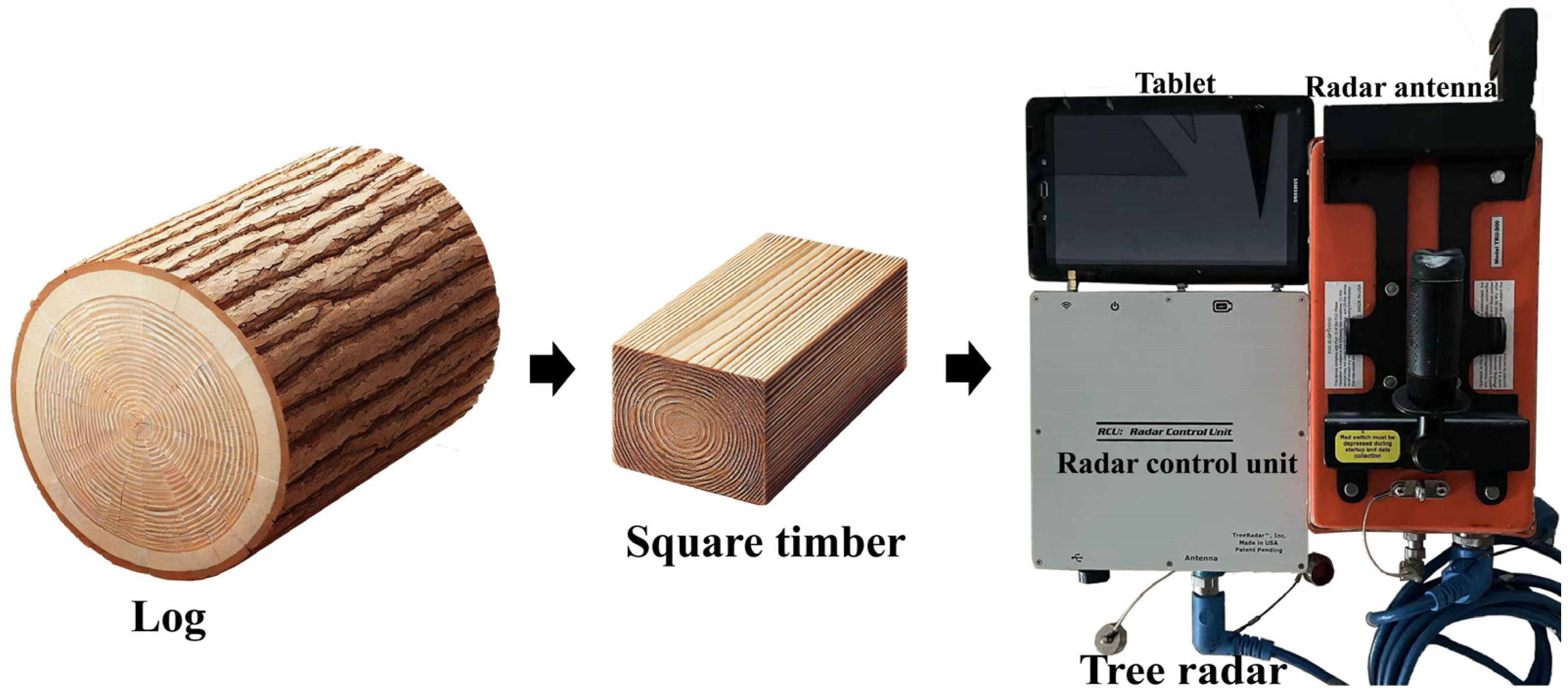
2.1. GPR Data Acquisition

This study selected wood samples (a thickness of approximately 20 cm) from four tree species, namely red spruce (Picea rubens), Dahurian larch (Larix gmelinii), European white birch (Betula pubescens), and Manchurian ash (Fraxinus mandshurica). They were obtained from 16 freshly harvested green logs, with the four selected species chosen for their significant economic importance in northeast China. The diameters of wood samples ranged from 25–30 cm, respectively. At the lumber mill, the logs were processed by cutting along their sides to produce 16 square timbers, each approximately 16 × 16 × 20 cm in size. To detect the MC of the wood samples, a tree radar developed based on GPR signals was utilized, which comprises three main components: a radar tablet that serves as a stable operational platform, a radar control unit that manages signal processing and system control, and a radar antenna that is responsible for transmitting and receiving GPR signals (Figure 1). The square timbers were soaked in water for over 30 days, and the changes in MC were measured by weighing. Subsequently, a tree radar (TRU-900) with some setting parameters such as frequency 900 MHz, radar gain 0, and dielectric constant 10 was used to obtain B-scan signals on the side of each square timber from four different directions [3]. Afterward, the samples were dried at 105 °C until the weight dropped by 100–200 g. The square timbers were then removed, re-weighed, and the B-scan signals were measured until the weight of the wood samples no longer changed during the drying process. Each square timber was weighed between 23 to 45 times. This method was employed to gather more MC data during the drying process, thereby enhancing the model’s generalization and robustness. Finally, the MC of square timbers was calculated using Equation (1).

Figure 1. Flowchart for detecting moisture content in square timber using tree radar.

Figure 1. Flowchart for detecting moisture content in square timber using tree radar.

$$MC={\displaystyle \frac{M_1-M_2}{M_2}}\times 100\%$$

(1)

M₁ is the wet weight and M₂ is the dry weight of the square timbers.

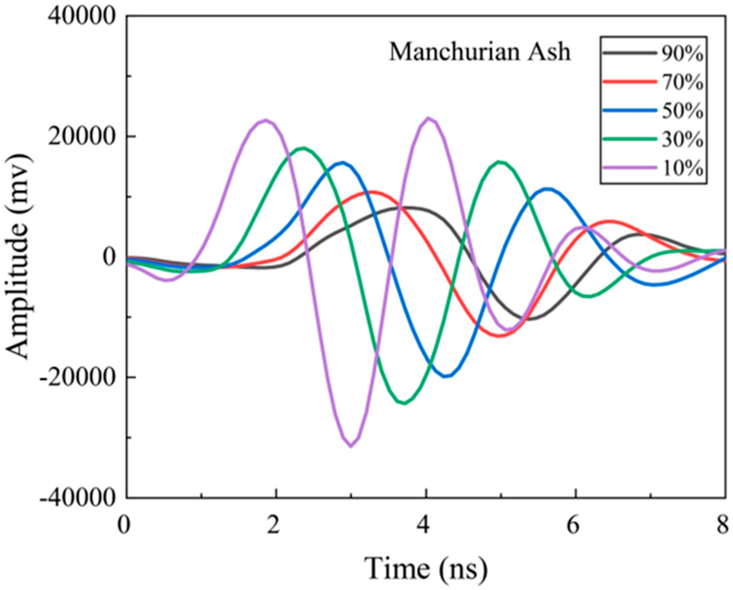
2.2. Signal Feature Analysis

A MATLAB R2022b program was designed based on the MATGPR_R1 software to extract the amplitude data within the GPR time domain signal matrix for the first 8 nanoseconds (including the first and second peaks and troughs) from the middle trace of the B-scan signals. Figure 2 demonstrates that the peaks and troughs of electromagnetic wave amplitudes vary with different MC levels. Higher MC suppresses wave propagation, resulting in lower amplitude values, while lower MC leads to greater amplitude variations. Additionally, varying MC affects the propagation time of electromagnetic waves. When the MC is higher, the peaks and troughs of the waveforms shift to the right on the time axis relative to those with lower MC, indicating a certain degree of delay. This delay occurs because higher MC slows down the wave speed, causing the peaks and troughs to be delayed on the time axis. Hence, it is evident that changes in MC affect not only the amplitude of the electromagnetic waves but also their propagation speed and phase. This finding is consistent with the results reported by Hans et al. (2015) [22], who investigated moisture content detection in logs with varying levels of MC. Previous studies have shown that the early-time portion of the GPR signal, which includes the direct air and ground wave events, is influenced by the shallow subsurface bulk electromagnetic properties of the material. These properties are strongly governed by the water content within the material [31]. It is primarily because the dielectric constant of water (80) is significantly higher than that of materials like wood. This highlights the impact of MC on the dielectric properties of square timber and further suggests that the amplitude information of electromagnetic waveforms can be utilized to predict the MC of square timber.

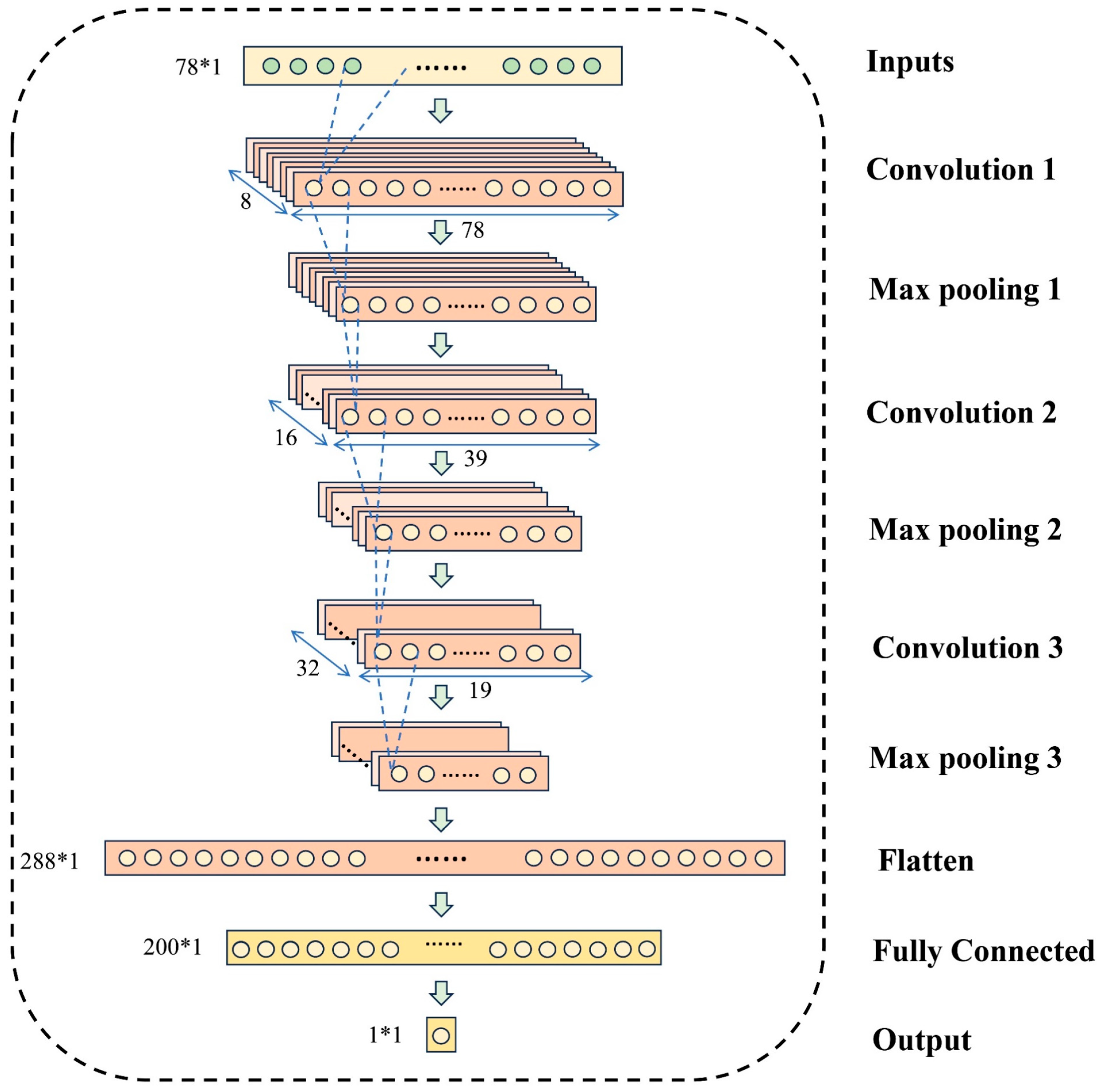
2.3. 1D-CNN Model Construction

Previous studies have often extracted some feature parameters from the GPR signals and used certain features for regression analysis [14]. However, this process only captures a part of the information about MC and increases the task complexity. 1D-CNN (one-dimensional convolutional neural network) exhibits excellent autonomous feature extraction capabilities and strong regression prediction performance. Therefore, in this study, the amplitude data for the first 8 nanoseconds was used as training feature parameters for MC prediction. By employing this approach, it becomes possible to fully utilize the available information contained in the GPR signals, which can enhance both the efficiency and accuracy of MC predictions.

In this study, the 1D-CNN architecture is presented for MC detection by GPR signals (Figure 3). The network starts with an input layer of dimension 78 × 1, representing the input feature vector derived from the full-waveform amplitude data of the GPR signals. The first convolutional layer comprises 8 filters, each of size 3, capturing local patterns in the input data through convolution operations.

$$y(i)=\sum _{j=0}^{k-1}x(i+j)\times w(j)+b$$

(2)

where $y$ is the output, $x$ is the input, $w$ is the convolution kernel, $k$ is the kernel size, and $j$ is the index within the convolution kernel.

Following this, a max-pooling layer with a pooling size of 2 reduces the dimensionality of the feature maps to 39 × 8.

$$y(i)={\max }_{j=0}^{k-1}x(i\times s+j)$$

(3)

where $s$ is the stride and $k$ is the pooling window size, and $j$ is the index within the pooling window.

The second convolutional layer utilizes 16 filters of size 3 to further extract complex features from the reduced feature maps, followed by another max-pooling layer with a pooling size of 2, reducing the feature map dimensions to 19 × 16. The third convolutional layer employs 32 filters of size 5 for additional convolution operations followed by a max-pooling layer with a pooling size of 2, resulting in feature maps of 9 × 32. A dropout layer with a rate of 0.5 is then applied to prevent overfitting. The output is flattened into a single vector of length 288 × 1, preparing it for the fully connected layers. This vector passes through a fully connected layer with 200 neurons.

$$y=Wx+b$$

(4)

where $y$ is the output vector, $W$ is the weight matrix, $x$ is the input vector, and $b$ is the bias vector. Finally, the output layer consists of a single neuron (1 × 1) that predicts the MC. To enhance model stability and accelerate convergence, batch normalization is applied after each pooling layer. The rectified linear unit (ReLU) activation function is used in all convolutional layers to introduce nonlinearity into the model, enabling it to learn complex patterns.

Figure 3. Flowchart of the 1D-CNN algorithm based on full-waveform amplitude data from GPR signals.

Figure 3. Flowchart of the 1D-CNN algorithm based on full-waveform amplitude data from GPR signals.

For the mixed species models, 2210 MC data samples were utilized. The MC data was randomly divided into 70% for training the neural network and 30% for testing its performance. The training and testing set distribution statistics for square timber MC across the 1D-CNN mixed-species models exhibited similar mean, median, and standard deviation values, indicating that the random partitioning result effectively represented the overall distribution (Table 1). Meanwhile, the feature parameters were standardized to ensure stability and convergence during model training.

Table 1. Summary statistics of the moisture content of square timber samples.

Category	Dataset	Min (%)	Max (%)	Mean (%)	Median (%)	Std (%)	Number
Mixed-species	All selected set	0	133.1	53.5	51	34.2	2208
	Training set	0	133.1	53.5	51	34.4	1545
	Testing set	0	133.1	53.7	51	33.8	663
Red spruce	All selected set	0	106.8	50.4	49.0	31.4	568
	Training set	0	106.8	50.2	48.9	32.2	397
	Testing set	0	104.1	51.1	49.1	29.5	171
Dahurian larch	All selected set	0	107	46.4	44.4	30.6	404
	Training set	0	107	46.1	44.4	29.9	283
	Testing set	0	107	47.1	44.4	32.2	122
White birch	All selected set	0	133.1	61.7	60.5	39.2	596
	Training set	0	133.1	61.7	59.2	38.4	417
	Testing set	0	133.1	61.6	61.3	41.1	179
Manchurian ash	All selected set	0	110.6	53.2	51.7	32.3	640
	Training set	0	110.6	52.9	51	32.2	448
	Testing set	0	110.6	53.8	51.7	32.8	192

Table 1. Summary statistics of the moisture content of square timber samples.

Category	Dataset	Min (%)	Max (%)	Mean (%)	Median (%)	Std (%)	Number
Mixed-species	All selected set	0	133.1	53.5	51	34.2	2208
	Training set	0	133.1	53.5	51	34.4	1545
	Testing set	0	133.1	53.7	51	33.8	663
Red spruce	All selected set	0	106.8	50.4	49.0	31.4	568
	Training set	0	106.8	50.2	48.9	32.2	397
	Testing set	0	104.1	51.1	49.1	29.5	171
Dahurian larch	All selected set	0	107	46.4	44.4	30.6	404
	Training set	0	107	46.1	44.4	29.9	283
	Testing set	0	107	47.1	44.4	32.2	122
White birch	All selected set	0	133.1	61.7	60.5	39.2	596
	Training set	0	133.1	61.7	59.2	38.4	417
	Testing set	0	133.1	61.6	61.3	41.1	179
Manchurian ash	All selected set	0	110.6	53.2	51.7	32.3	640
	Training set	0	110.6	52.9	51	32.2	448
	Testing set	0	110.6	53.8	51.7	32.8	192

$$P_{\mathrm{standard}}={\displaystyle \frac{P-P_{\mathrm{mean}}}{P_{\mathrm{std}}}}$$

(5)

$P_{\mathrm{standard}}$ is the standardized value, $p$ is the original value, $P_{\mathrm{mean}}$ and $P_{\mathrm{std}}$ are the mean and standard deviation of the feature, respectively.

For the objective function, mean squared error was chosen to describe the difference between the predicted value and the true value.

$$\mathrm{Loss}={\displaystyle \frac{1}{n}}\sum _{i=1}^n{(y_i-{\widehat{y}}_i)}^2$$

(6)

where $n$ is the number of samples, $y_i$ and ${\widehat{y}}_i$ are the true and predicted values for the i-th sample.

Based on experience and multiple attempts, the mixed species model was trained using the Adam optimizer with a learning rate of 0.001 for 300 epochs to minimize the loss value.

2.4. Comparative Analysis of Different Algorithms for Time–Frequency Parameters and Full-Waveform Amplitude Based on GPR Signals

To evaluate the effectiveness of time–frequency parameters and full-waveform amplitude, A MATLAB program was designed based on the MATGPR software to extract time–frequency parameters from GPR signals, comprising 19 time domain parameters and 12 frequency domain parameters (

Table 2. Time–frequency parameters for square timber moisture content.

Time Domain Parameters				Frequency Domain Parameters
Name	Explanation	Name	Explanation	Name	Explanation
Maximum	$P_1=\max \left(X_i\right)$	Standard deviation	$P_{13}=\sqrt{{\displaystyle \frac{1}{n-1}}{\displaystyle \sum _{i=1}^n{\left(X_i-P_3\right)}^2}}$	Amplitude average	$P_{20}={\displaystyle \frac{1}{m}}{\displaystyle \sum _{k=1}^{m}s\left(k\right)}$
Minimum	$P_2=\min \left(X_i\right)$	Skewness coefficient	$P_{14}={\displaystyle \frac{P_7}{\left(n-1\right){P_{13}}^3}}$	Amplitude standard deviation	$P_{21}=\sqrt{{\displaystyle \frac{1}{m-1}}{\displaystyle \sum _{k=1}^m{\left(s\left(k\right)-P_{20}\right)}^2}}$
Mean	$P_3={\displaystyle \frac{1}{n}}{\displaystyle \sum _{i=1}^n{X}_i}$	Kurtosis coefficient	$P_{15}={\displaystyle \frac{P_8}{\left(n-1\right){P_{13}}^4}}$	Sample Skewness	$P_{22}={\displaystyle \frac{{\displaystyle \sum _{k=1}^m{\left(s\left(k\right)-P_{20}\right)}^3}}{\left(m-1\right){P_{21}}^3}}$
Average absolute value	$P_4={\displaystyle \frac{1}{n}}{\displaystyle \sum _{i=1}^n\left|X_i\right|}$	Peak factor	$P_{16}={\displaystyle \frac{P_1}{P_9}}$	Sample Kurtosis	$P_{23}={\displaystyle \frac{{\displaystyle \sum _{k=1}^m{\left(s\left(k\right)-P_{20}\right)}^4}}{\left(m-1\right){P_{21}}^4}}$
Peak-to-peak value	$P_5=\max \left(X\right)-\min \left(X\right)$	Peak-to-mean ratio	$P_{17}={\displaystyle \frac{P_1}{P_{10}}}$	Frequency mean	$P_{24}={\displaystyle \frac{{\displaystyle \sum _{k=1}^m{f}_{k}s\left(k\right)}}{{\displaystyle \sum _{k=1}^{m}s\left(k\right)}}}$
Variance	$P_6={\displaystyle \frac{1}{n}}{\displaystyle \sum _{i=1}^n{\left(X_i-P_3\right)}^2}$	Form factor	$P_{18}={\displaystyle \frac{P_9}{P_4}}$	Frequency standard deviation	$P_{25}=\sqrt{{\displaystyle \frac{{\displaystyle \sum _{k=1}^m{\left(f_k-P_{24}\right)}^{2}s\left(k\right)}}{K}}}$
Skewness	$P_7={\displaystyle \frac{1}{n}}{\displaystyle \sum _{i=1}^n{\left(X_i-P_3\right)}^3}$	Amplitude factor	$P_{19}={\displaystyle \frac{P_1}{P_4}}$	Frequency Root Mean Square	$P_{26}=\sqrt{{\displaystyle \frac{{\displaystyle \sum _{k=1}^m{f_k}^{2}s\left(k\right)}}{{\displaystyle \sum _{k=1}^{m}s\left(k\right)}}}}$
Kurtosis	$P_8={\displaystyle \frac{1}{n}}{\displaystyle \sum _{i=1}^n{\left(X_i-P_3\right)}^4}$			Frequency Fourth Root Mean Square	$P_{27}=\sqrt{{\displaystyle \frac{{\displaystyle \sum _{k=1}^m{f_k}^{4}s\left(k\right)}}{{\displaystyle \sum _{k=1}^m{f_k}^{2}s\left(k\right)}}}}$
Root mean square	$P_9=\sqrt{{\displaystyle \frac{1}{n}}{\displaystyle \sum _{i=1}^n{X_i}^2}}$			Frequency Band Index	$P_{28}={\displaystyle \frac{{\displaystyle \sum _{k=1}^m{f_k}^{2}s\left(k\right)}}{\sqrt{{\displaystyle \sum _{k=1}^{m}s\left(k\right)}{\displaystyle \sum _{k=1}^m{f_k}^{4}s\left(k\right)}}}}$
Mean square amplitude	$P_{10}={\left({\displaystyle \frac{1}{n}}{\displaystyle \sum _{i=1}^n\sqrt{\left|X_i\right|}}\right)}^2$			Frequency Bandwidth Index	$P_{29}={\displaystyle \frac{P_{25}}{P_{24}}}$
Total energy	$P_{11}={\displaystyle \sum _{i=1}^n{X_i}^2}$			Frequency skewness	$P_{30}={\displaystyle \frac{{\displaystyle \sum _{k=1}^m{\left(f_k-P_{21}\right)}^{3}s\left(k\right)}}{m\times {P_{25}}^3}}$
Average energy	$P_{12}={\displaystyle \frac{1}{n}}{\displaystyle \sum _{i=1}^n{X_i}^2}$			Frequency kurtosis	$P_{31}={\displaystyle \frac{{\displaystyle \sum _{k=1}^m{\left(f_k-P_{21}\right)}^{4}s\left(k\right)}}{m\times {P_{25}}^4}}$

Note: x_i is the i-th sample point of a GPR trace and i = 1, 2, …, n, n is the sample point per trace, and s(k) is the frequency amplitude transformed from the GPR trace by the Fast Fourier Transform method, k = 1, 2, …, m, m is the number of frequency components, and $f_k$ is the k-th frequency component.

).

In forestry applications, random forest (RF), k-nearest neighbors (KNN), and back propagation neural network (BPNN) are widely used machine learning algorithms. RF enhances model performance by integrating multiple decision trees [32], whereas KNN makes predictions based on the distance between samples [33], and BPNN adjusts to complex relationships through backpropagation training [3]. Partial Least Squares (PLS) is a widely used statistical method in forestry that constructs predictive models by simultaneously considering the covariance between independent and dependent variables [22]. This method is particularly well-suited for handling high-dimensional datasets and situations with significant multicollinearity. In this study, to determine the most effective algorithm for MC detection, these models were compared with 1D-CNN models. The same training and testing sets were utilized, and a 5-fold cross-validation with grid search was performed to determine their optimal hyperparameters (

Table 3. Predictive performance of 1D-CNN, RF, KNN, and BPNN models based on full-waveform amplitude and time–frequency domain parameters for square timber in the training and testing sets.

Parameter Class	Model	Hyperparameter Values	Testing Set			Training Set
			R2	RMSE	MAE	R2	RMSE	MAE
Full waveform amplitude	1D-CNN	epochs = 300, batch_size = 16.	0.9864	0.0393	0.0298	0.9907	0.0332	0.0255
	RF	n_estimators:900, max_depth: 9.	0.9799	0.0479	0.0329	0.9972	0.0181	0.0122
	KNN	n_neighbors: 3.	0.9837	0.0430	0.0265	0.9945	0.0253	0.0151
	BPNN	hidden_layer: (30,15) activation: relu.	0.9686	0.0598	0.0446	0.9792	0.0496	0.0378
	PLS	n_components: 14.	0.9111	0.1006	0.0785	0.9189	0.0980	0.0755
Time–frequency domain parameters	RF	n_estimators:300, max_depth:9.	0.9382	0.0840	0.0589	0.9917	0.0314	0.0224
	KNN	n_neighbors: 5.	0.9254	0.0922	0.0620	0.9528	0.0747	0.0490
	BPNN	hidden_layer: (20) activation: tanh.	0.9130	0.0994	0.0748	0.9336	0.0886	0.0666
	PLS	n_components: 14.	0.8469	0.1345	0.1060	0.8543	0.1289	0.1013

).

2.5. Square Timber MC Models for Different Tree Species

Previous studies have demonstrated that single-species models exhibit higher predictive accuracy compared to mixed-species models [3,22]. Therefore, to further enhance detection accuracy, four 1D-CNN single-species models were developed in this study by classifying into four species groups: Red spruce with 568 MC data ranging from 0% to 133.1% MC, Dahurian larch with 404 MC data ranging from 0% to 107% MC, European white birch with 596 MC data ranging from 0% to 133.1% MC, and Manchurian ash with 640 MC data ranging from 0.1% to 110.6% MC. The training and testing set distribution statistics for square timber MC across the four 1D-CNN single-species models also exhibited similar mean, median, and standard deviation values, indicating that the random partitioning result effectively represented the overall distribution (Table 1). Based on experience and multiple attempts, the 1D-CNN single-species models were trained with a batch size range of 4–8 (

Table 4. Predictive performance of 1D-CNN models based on full waveform amplitude for square timber of different tree species in training and testing sets.

Category	Hyperparameter Values	Testing Set			Training Set
		R2	RMSE	MAE	R2	RMSE	MAE
Red spruce	epochs = 300, batch_size = 4.	0.9902	0.0320	0.0263	0.9915	0.0284	0.0225
Dahurian larch	epochs = 300, batch_size = 4.	0.9876	0.0358	0.0282	0.9893	0.0310	0.0242
European white birch	epochs = 300, batch_size = 8.	0.9930	0.0343	0.0269	0.9942	0.0291	0.0237
Manchurian ash	epochs = 300, batch_size = 4.	0.9931	0.0271	0.0215	0.9939	0.0251	0.0197

), using the Adam optimizer with a learning rate of 0.001 for 300 epochs to minimize the loss value.

3. Result and Discussion

3.1. Construction of 1D-CNN for Mixed-Species Trees

The training and testing loss curves for the 1D-CNN mixed-species model quickly decreased and stabilized, indicating consistent and effective performance across both sets without overfitting (Figure 4a). The model demonstrated high predictive accuracy, with an R² value of 0.9864 and an RMSE of 0.0393 (Table 3). The MAE was 0.0298, and the maximum residuals were below 18%. Notably, the residuals remained particularly low under 8% for MC below 40% (Figure 4b), highlighting the model’s effectiveness in practical applications. When the MC exceeds 50%, the primary cause of increased model prediction errors may be due to the further increase in the wood’s MC, which results in a continuous increase in the dielectric constant. This change may significantly slow the propagation of electromagnetic waves, enhance signal attenuation, and increase noise levels, leading to greater prediction errors (Figure 2).

3.2. Comparison of Different Algorithms for Time–Frequency Parameters and Full-Waveform Amplitude from GPR Signals

A systematic comparative analysis was conducted on five models: 1D-CNN, RF, KNN, BPNN, and PLS using full-waveform amplitude from GPR signals. The results indicated that the 1D-CNN model demonstrated superior performance, followed by KNN (R² = 0.9837, RMSE = 0.0430) and RF (R² = 0.9799, RMSE = 0.0479). While BPNN showed relatively lower predictive accuracy (R² = 0.9686, RMSE = 0.0598), PLS exhibited the poorest performance (R² = 0.9111, RMSE = 0.1006). These findings highlight the significant advantage of 1D-CNN in processing full-waveform amplitude data. The model’s automatic and hierarchical feature extraction effectively captures both local and global features [34], thereby markedly improving prediction accuracy. In contrast, the PLS model is constrained by its linear characteristics, making it less effective in capturing the nonlinear relationships in GPR full-waveform amplitude data. The KNN model leverages distance metrics to capture local patterns in the full-waveform amplitude data, achieving high prediction accuracy [33]. This indicates that GPR full-waveform amplitude data possess significant local characteristics. Moreover, the RF model efficiently captures the complex nonlinear relationships within GPR full-waveform amplitude data by constructing multiple decision trees, leading to relatively stable predictive performance [32]. The relatively lower accuracy of the BPNN can be attributed to its simpler architecture, which constrains its capability to capture intricate patterns in the data.

Compared to the algorithm based on full-waveform amplitude data, the algorithm based on the time–frequency parameters exhibited significantly lower model performance (Table 3). This may be attributed to the inability of time–frequency parameters to comprehensively capture the complete information of the GPR signals, leading to the omission of critical features during model training. These findings indicate that the method based on full-waveform amplitude data is more advantageous and applicable for detecting wood MC using GPR signals.

3.3. D-CNN Model Construction for Different Tree Species

The training and testing loss curves for the 1D-CNN models in Red spruce, Dahurian larch, European white birch, and Manchurian ash exhibited a rapid decrease followed by stabilization, indicating robust and consistent performance across both sets without overfitting (Figure 5a,c,e,g). The prediction performance of models for individual tree species surpassed that of the mixed-species model (R² ≥ 0.9876, RMSE ≤ 0.0358), which is consistent with previous research findings [3,22]. This finding underscores the significant structural and density differences among tree species, which affect the propagation of electromagnetic waves to varying degrees. To improve prediction accuracy in practical industrial applications, specialized models for specific tree species should be utilized, fully considering the physical characteristics of different species and incorporating more experimental data for training. Among the species, Manchurian ash achieved the highest prediction accuracy (R² = 0.9931, RMSE = 0.0271), followed by European white birch (R² = 0.9930, RMSE = 0.0343) and red spruce (R² = 0.9902, RMSE = 0.0320), whereas the accuracy for Dahurian larch was relatively lower (Table 4). This may be attributed to the smaller sample size for Dahurian larch, which did not completely meet the larger data requirements for training the 1D-CNN model, thereby resulting in reduced prediction accuracy for this species. Therefore, it is necessary to increase the sample size for Dahurian larch in particular to enhance the generalization and predictive accuracy of the 1D-CNN model. According to Figure 5b,d,f,h, the residuals for all models were almost within 10%. When the MC was below 40%, the residuals for other models were almost within 5%, except for Dahurian larch. This indicates that single-species models are more accurate at low MC, further validating their effectiveness in practical detection applications.

The 1D-CNN MC prediction models for square timber exhibit significant potential in the wood drying process. The single-species model offers higher accuracy for specific wood types, making it suitable for precise applications, while the mixed-species model provides greater efficiency and adaptability across various scenarios. These models enable real-time monitoring of wood MC, optimizing drying processes and enhancing efficiency. Moreover, they have potential applications in MC detection of load-bearing wood in construction and bridge engineering, aiding in the formulation of quality control measures. Our further research will aim to include more tree species, gather more experimental data, further optimize the algorithms, and validate these models in actual industrial production to enhance their applicability and reliability.

4. Conclusions

This study developed a 1D-CNN model to predict the MC of square timbers from red spruce, Dahurian larch, European white birch, and Manchurian ash (MC range 0%–133.1%) using the first 8 nanoseconds of GPR signals. The mixed-species model demonstrated effective predictive performance, with an R² value of 0.9864 and an RMSE of 0.0393, indicating the 1D-CNN model’s superior capability in handling complex data. Single-species models exhibited even higher predictive performance (R² ≥ 0.9876, RMSE ≤ 0.0358), particularly for species such as red spruce, European white birch, and Manchurian ash. This suggests that density and structural differences among tree species significantly affect electromagnetic wave propagation. Therefore, different models can be employed to achieve optimal results in specific application requirements. Additionally, the study found that the algorithms based on full-waveform amplitude data have a significant advantage in detecting wood MC compared to those using multi time–frequency parameters, and the 1D-CNN model can automatically extract both linear and nonlinear features hierarchically, showing higher predictive accuracy compared to other algorithms. These findings have significant importance for real-time monitoring of the wood drying process and the MC detection of load-bearing wood in construction and bridge engineering. Future research will expand the range of tree species and increase the sample size to further enhance the model’s applicability and reliability.

References

1. Forsén, H.; Tarvainen, V. Accuracy and Functionality of Hand Held Wood Moisture Content Meters; Technical Research Centre of Finland: Espoo, Finland, 2000; pp. 2–79. [Google Scholar]
2. Redman, J.; Hans, G.; Diamanti, N. Impact of Wood Sample Shape and Size on Moisture Content Measurement Using a GPR-Based Sensor. IEEE J.-STARS 2016, 9, 221–227. [Google Scholar] [CrossRef]
3. Guo, J.; Wang, P.; Qin, R.; Zhao, L.; Tang, X.; Zeng, J.; Xu, H. Detection of moisture content in logs using multi-parameter GPR signal analysis and neural network models. Holzforschung 2023, 77, 240–247. [Google Scholar] [CrossRef]
4. Gereke, T.; Hass, P.; Niemz, P. Moisture-induced stresses and distortions in spruce cross-laminates and composite laminates. Holzforschung 2010, 64, 127–133. [Google Scholar] [CrossRef]
5. Hänsel, A.; Sandak, J.; Sandak, A.; Mai, J.; Niemz, P. Selected previous findings on the factors influencing the gluing quality of solid wood products in timber construction and possible developments: A review. Wood Mater. Sci. Eng. 2022, 17, 230–241. [Google Scholar] [CrossRef]
6. Govett, R.; Mace, T.; Bowe, S. A Practical Guide for the Determination of Moisture Content of Woody Biomass; University of Wisconsin: Madison, WI, USA, 2010; Volume 20. [Google Scholar]
7. Dietsch, P.; Franke, S.; Franke, B.; Gamper, A.; Winter, S. Methods to determine wood moisture content and their applicability in monitoring concepts. J. Civ. Struct. Health Monit. 2015, 5, 115–127. [Google Scholar] [CrossRef]
8. Dahlen, J.; Schimleck, L.; Schilling, E. Modeling and Monitoring of Wood Moisture Content Using Time-Domain Reflectometry. Forests 2020, 11, 479. [Google Scholar] [CrossRef]
9. Dos Santos, L.M.; Amaral, E.A.; Nieri, E.M.; Costa, E.V.S.; Trugilho, P.F.; Calegário, N.; Hein, P.R.G. Estimating wood moisture by near infrared spectroscopy: Testing acquisition methods and wood surfaces qualities. Wood Mater. Sci. Eng. 2021, 16, 336–343. [Google Scholar] [CrossRef]
10. Sharma, A.; Singh, B.; Sandhu, B.S. A gamma-ray scattering technique for estimation of density and moisture content of wood. Radiat. Eff. Defects Solids 2017, 172, 286–295. [Google Scholar] [CrossRef]
11. He, X.; Qi, D. Density and moisture content forecasting based on X-ray computed tomography. Eur. J. Wood Wood Prod. 2013, 71, 647–652. [Google Scholar] [CrossRef]
12. Wolter, B.; Krus, M. Moisture Measuring with Nuclear Magnetic Resonance (NMR). In Electromagnetic Aquametry: Electromagnetic Wave Interaction with Water and Moist Substances; Kupfer, K., Ed.; Springer: Berlin/Heidelberg, Germany, 2005; pp. 491–515. [Google Scholar]
13. Pajewski, L.; Benedetto, A.; Derobert, X.; Giannopoulos, A.; Loizos, A.; Manacorda, G.; Marciniak, M.; Plati, C.; Schettini, G.; Trinks, I. Applications of Ground Penetrating Radar in civil engineering—COST action TU1208. In Proceedings of the 2013 7th International Workshop on Advanced Ground Penetrating Radar, Nantes, France, 2–5 July 2013; pp. 1–6. [Google Scholar]
14. Zhang, J.; Zhang, C.; Lu, Y.; Zheng, T.; Dong, Z.; Tian, Y.; Jia, Y. In-situ recognition of moisture damage in bridge deck asphalt pavement with time-frequency features of GPR signal. Constr. Build. Mater. 2020, 244, 118295. [Google Scholar] [CrossRef]
15. Sbartaï, Z.M.; Laurens, S.; Balayssac, J.P.; Arliguie, G.; Ballivy, G. Ability of the direct wave of radar ground-coupled antenna for NDT of concrete structures. NDT&E Int. 2006, 39, 400–407. [Google Scholar]
16. Li, F.; Yang, F.; Qiao, X.; Hu, Z.; Wu, X.; Xing, H. 3D ground penetrating radar road underground target identification algorithm using time-frequency statistical features of data. NDT&E Int. 2023, 137, 102860. [Google Scholar]
17. Shirmohammadi, M.; Leggate, W.; Redman, A. Effects of moisture ingress and egress on the performance and service life of mass timber products in buildings: A review. Constr. Build. Mater. 2021, 290, 123176. [Google Scholar] [CrossRef]
18. Mai, T.C.; Razafindratsima, S.; Sbartaï, Z.M.; Demontoux, F.; Bos, F. Non-destructive evaluation of moisture content of wood material at GPR frequency. Constr. Build. Mater. 2015, 77, 213–217. [Google Scholar] [CrossRef]
19. Rodríguez-Abad, I.; Martínez-Sala, R.; García-García, F.; Capuz-Lladró, R. Ability of the Direct Wave Amplitude of Ground-penetrating Radar for Assessing the Moisture Content Variation of Timber. In Proceedings of the 16th EAGE European Meeting of Environmental and Engineering Geophysics, Zurich, Switzerland, 6–8 September 2010; pp. 2214–4609. [Google Scholar]
20. Rodríguez-Abad, I.; Martínez-Sala, R.; García-García, F.; Capuz-Lladró, R. Non-destructive methodologies for the evaluation of moisture content in sawn timber structures: Ground-penetrating radar and ultrasound techniques. Near Surf. Geophys. 2010, 8, 475–482. [Google Scholar] [CrossRef]
21. Marques Duarte da Paz, A.M. Water Content Measurement in Woody Biomass: Using Dielectric Constant at Radio Frequencies. Ph.D. Thesis, Mälardalen University, Västerås, Sweden, 2008. [Google Scholar]
22. Hans, G.; Redman, D.; Leblon, B.; Nader, J.; La Rocque, A. Determination of log moisture content using early-time ground penetrating radar signal. Wood Mater. Sci. Eng. 2015, 10, 112–129. [Google Scholar] [CrossRef]
23. Zhang, W.; Yan, J.; Yan, Y. Measurement of the moisture content in woodchips through capacitive sensing and data driven modelling. Measurement 2021, 186, 110205. [Google Scholar] [CrossRef]
24. Zheng, S.; Gao, P.; Wang, W.; Zou, X. A Highly Accurate Forest Fire Prediction Model Based on an Improved Dynamic Convolutional Neural Network. Appl. Sci. 2022, 12, 6721. [Google Scholar] [CrossRef]
25. You, X.; Zheng, Z.; Yang, K.; Yu, L.; Liu, J.; Chen, J.; Lu, X.; Guo, S. A PSO-CNN-Based Deep Learning Model for Predicting Forest Fire Risk on a National Scale. Forests 2024, 15, 86. [Google Scholar] [CrossRef]
26. Egli, S.; Höpke, M. CNN-Based Tree Species Classification Using High Resolution RGB Image Data from Automated UAV Observations. Remote Sens. 2020, 12, 3892. [Google Scholar] [CrossRef]
27. Jiao, L.; Dong, S.; Zhang, S.; Xie, C.; Wang, H. AF-RCNN: An anchor-free convolutional neural network for multi-categories agricultural pest detection. Comput. Electron. Agric. 2020, 174, 105522. [Google Scholar] [CrossRef]
28. Kiranyaz, S.; Ince, T.; Hamila, R.; Gabbouj, M. Convolutional Neural Networks for patient-specific ECG classification. In Proceedings of the 2015 37th Annual International Conference of the IEEE Engineering in Medicine and Biology Society (EMBC), Milan, Italy, 25–29 August 2015; pp. 2608–2611. [Google Scholar]
29. Zheng, J.; Teng, X.; Liu, J.; Qiao, X. Convolutional Neural Networks for Water Content Classification and Prediction with Ground Penetrating Radar. IEEE Access 2019, 7, 185385–185392. [Google Scholar] [CrossRef]
30. Xu, J.; Zhang, J.; Sun, W. Recognition of the Typical Distress in Concrete Pavement Based on GPR and 1D-CNN. Remote Sens. 2021, 13, 2375. [Google Scholar] [CrossRef]
31. Ferrara, C.; Barone, P.M.; Steelman, C.M.; Pettinelli, E.; Endres, A.L. Monitoring Shallow Soil Water Content Under Natural Field Conditions Using the Early-Time GPR Signal Technique. Vadose Zone J. 2013, 12, vzj2012.0202. [Google Scholar] [CrossRef]
32. Su, H.; Shen, W.; Wang, J.; Ali, A.; Li, M. Machine learning and geostatistical approaches for estimating aboveground biomass in Chinese subtropical forests. For. Ecosyst. 2020, 7, 64. [Google Scholar] [CrossRef]
33. Shin, J.; Temesgen, H.; Strunk, J.L.; Hilker, T. Comparing modeling methods for predicting forest attributes using LiDAR metrics and ground measurements. Can. J. Remote Sens. 2016, 42, 739–765. [Google Scholar] [CrossRef]
34. Zheng, Y.; Huang, J.; Chen, T.; Ou, Y.; Zhou, W. CNN classification based on global and local features. In Proceedings of the Real-Time Image Processing and Deep Learning 2019, Baltimore, MD, USA, 14–18 April 2019; pp. 96–108. [Google Scholar]
Figure 2. Electromagnetic wave time domain variations at different moisture content levels (10%–90%) for Manchurian ash square timbers, with an error range of ±0.5%.
Forests 15 01800 g002
Figure 4. 1D-CNN model loss curves (a) and residuals (b) for moisture content in mixed-species square timber.
Forests 15 01800 g004
Figure 5. 1D-CNN model loss curves (a,c,e,g) and residuals (b,d,f,h) for moisture content in red spruce, Dahurian larch, European white birch, and Manchurian ash square timbers.
Forests 15 01800 g005