Leaf Moisture Content Detection Method Based on UHF RFID and Hyperdimensional Computing

Abstract

Leaf moisture content (LMC) directly affects the life activities of plants and becomes a key factor to evaluate the growth status of plants. To explore a low-cost, real-time, rapid, and accurate method for LMC detection, this paper employs Ultra-High-Frequency Radio-Frequency Identification (UHF RFID) sensor technology. By reading the tag information attached to the back of leaves, the parameters of the RSSI, phase, and reading distance of the tags are collected. In this paper, we propose an enhanced Multi-Feature Fusion algorithm based on Hyperdimensional Computing (HDC) called MFFHDC. In our proposed method, the real-valued features are encoded into hypervectors and then combined with Multi-Linear Discriminant Analysis (MLDA) for the feature fusion of different features. Finally, a retraining method based on Cosine Annealing with Warm Restarts (CAWR) is proposed to improve the model and further enhance its accuracy. Tests conducted in the experimental forest show that the proposed mechanism can effectively predict the LMC. The model’s Mean Absolute Error (MAE), Root Mean Square Error (RMSE), and Coefficient of Determination (R²) reached 0.0195, 0.0255, and 0.9131, respectively. Additionally, comparisons with other methods demonstrate that the presented system performs excellently in most aspects. As a lightweight model, this study shows great practical application value, particularly for the limited data volume and low hardware costs.

1. Introduction

The study of leaf moisture content (LMC) is vital for forestry and environmental science, playing a crucial role in optimizing irrigation and conserving water resources while ensuring healthy plant growth [1]. The LMC directly influences photosynthesis, respiration, and transpiration, which can be considered an important parameter for assessing plant growth and health status. In arid environments, reduced LMC affects the rate at which stomata absorb carbon dioxide and release oxygen, thereby decreasing the rate of photosynthesis and impacting plant growth and development. When water is insufficient, plant growth can be stunted, leading to delayed development, shorter stature, and reduced yield. Conversely, excessive water can not only degrade fruit quality but also make plants more susceptible to various diseases, ultimately affecting their overall health. The research of LMC is integral to the emerging field of the Forestry Internet of Things (FIoT) [2]. The traditional method for detecting LMC is the drying method [3]. This method involves measuring the weight of the sample before and after drying by placing the target sample in an oven and drying it multiple times until it reaches a constant weight. However, this method is cumbersome, cannot achieve online or real-time measurement, and causes damage to the sample itself.

In recent years, non-destructive testing methods have emerged, attracting wide-spread attention from researchers. S. Shen et al. [4] used a deep learning method to extract the characteristics of tea near-infrared spectra and measure the changes in the water content of black tea leaves during the withering process. Dong et al. established a moisture prediction model in the range of 400–1000 nm [5]. Under various actual environmental conditions, the problem of detecting LMC in stacks [6] and on conveyor belts simulating actual production conditions [7] was solved. Sun et al. used an optimization algorithm to select characteristic wavelengths and extracted near-infrared hyperspectral reflectance to enable visual research on the moisture content of tea leaves [8]. In [9], Liu et al. used hyperspectral imaging to measure the moisture content of rapeseed leaves, achieving a Root Mean Square Error (RMSE) of 0.0065. Li et al. used terahertz time-domain spectroscopy to detect the moisture content of soybeans [10].

Due to the high cost of hyperspectral imaging methods, many scholars have developed alternative approaches. For example, remote sensing methods have been explored [11]: Susan C. et al. [12] used the European Remote Sensing Wind Scatterometer to study water stress in vegetation. Basyigit I.B. et al. [13] established a moisture content prediction model based on the influence of banana LMC on remote sensing dielectric constant. Tang et al. used electrical impedance spectroscopy, selecting frequencies of different impedances and comparing several regression and deep learning algorithms, ultimately proving that the random forest algorithm performed best [14]. Abdul Jabbar et al. [15] designed a Lorentz resonator sensor based on the rapid slope change of the phase spectrum to measure the moisture content of leaves in a tree network environment. Han et al. [16] used a camera to capture leaf images and methods such as gray co-occurrence matrix and gray histogram to extract image features and analyze the correlation between these features and moisture content. In practical applications of spectral methods, such as hyperspectral imaging, a hyperspectral camera is typically used to capture spectral images of leaves to identify their moisture content. However, hyperspectral cameras are generally bulky, and expensive, and require external power sources. Additionally, they have strict requirements regarding the angle of capture.

More and more Internet-of-Things-related technologies are being applied in forestry research, such as plant type identification [17,18], crop picking identification [19], forest fire early warning [20,21,22], leaf disease, pest identification and prevention [23], etc. Shivling V.D. et al. [24] designed a patch antenna, where the resonant frequency changes with the moisture content, allowing for a predictive model to be established. Bekas et al. theoretically analyzed the radio-frequency signal absorption of banana leaves with different moisture contents [25]. Subsequently, Tein S.Y. et al. applied radio-frequency waveguide antennas [26]. Bo et al. [27] designed a wearable capacitive sensor to predict LMC. In the evolving landscape of the IoT, Radio-Frequency Identification (RFID) technology has emerged as a transformative force and made substantial inroads into the forestry sector, where it is catalyzing revolutionary advancements in forest management practices [28]. RFID’s ability to tag, track, and monitor assets in real time [29,30] provides forest managers with a powerful tool to optimize their operations. However, when paired with the detection of LMC, RFID in FIoT achieves an unprecedented level of sophistication and insight [31]. Based on the impact of moisture on radio-frequency signals, Joan et al. [32] attached tags at different locations on the vehicle and used the RFID method to measure the humidity at various locations. Wu and Zhang et al. [33] successfully measured the moisture content of living trees based on the RSSI and distance of the frequency signal activity based on the RSSI and distance of the radio-frequency signal.

As an emerging cognitive model, Hyperdimensional Computing (HDC) can be regarded as a form of high-dimensional global stochastic mapping and similarity matching [34]. In HDC, each information entity is encoded as a hypervector—a high-dimensional vector with thousands, tens of thousands, or even more dimensions into the hyperdimensional space through mapping. Various cognitive operations are then realized using the unique algorithms of HDC along with some subsequent processing. In 2009, Kanerva [35] integrated early models in vector symbolic architecture and formally proposed the systematic theory and basic principles of HDC in a tutorial article. Mohsen Imani et al. developed VoiceHD, a speech recognition system using HDC, which was further enhanced by a neural network layer in VoiceHD+NN. This system efficiently classifies voice signals and significantly outperforms traditional neural networks in speed and energy efficiency, making it ideal for IoT devices [36]. Due to its low cost, fast computation speed, and strong robustness, HDC has been applied in various fields such as speech recognition [37,38], biological signal processing [39,40], epilepsy detection [41], diabetes diagnosis [42], and human behavior recognition [43], and other fields have been widely used. Wang et al. developed a method using HDC for the real-time detection of electrical load anomalies in smart grids. The study demonstrated that HDC significantly improves detection accuracy and efficiency over traditional machine learning and deep learning methods [44]. In [45], Mohsen et al. proposed AdaptHD, which introduced learning rate into HDC for the first time and employs both iteration-dependent and data-dependent strategies to dynamically adjust the learning rate, significantly enhancing training speed and energy efficiency. Farhad T. et al. [46] proposed PartialHD, which divides a long hypervector into multiple partial vectors and processes each vector separately, improving accuracy by 1.93% during the retraining stage. Karunaratne, G et al. [47] introduced an in-memory HDC system leveraging the attributes of neuronal circuits such as hyperdimensionality and robustness to imperfections. This system uses phase-change memory (PCM) devices to perform analog in-memory computations for machine learning tasks. HDC has also achieved very good results on some devices with limited computing resources, such as FPGA [48], brain–computer interface [49], smartphones [50], etc. However, HDC has not yet been applied in the field of FIoT.

Addressing the issues of high cost, poor anti-interference performance, and low robustness in current LMC research methods, we aim to develop a method that provides real-time, on-site, fast, and accurate measurements in complex outdoor environments such as forests. As shown in Figure 1, this illustration represents our UHF-RFID-based LMC detection system.

Based on the research objectives, we propose the following initial hypotheses: (1) Different moisture contents will lead to changes in the dielectric constant of leaves, and, by detecting the dielectric properties of the leaves, machine learning algorithms can be used to infer the leaf moisture content. (2) Based on the sensitivity of UHF radio-frequency signals to moisture, by measuring the phase, RSSI, and reading the distance of the signals, the dielectric properties under different moisture contents can be quantified. (3) Other characteristics of the leaves (such as thickness, type, and salinity) may also affect the dielectric properties, and further research is needed to evaluate the impact of these factors. The specific research methods are as follows: (1) In the experimental forest, UHF RFID sensors were used to collect data on RSSI, phase, and reading/writing distance from multiple sets of fallen leaves, dead leaves, and fresh leaves, which served as the primary basis for determining leaf moisture content. (2) A preliminary model framework based on Hyperdimensional Computing (HDC) was established, where the measured real-valued features were encoded into hyperdimensional vectors, and cosine similarity was used to assess leaf moisture content. (3) To address the issue of feature entanglement, a multidimensional linear discriminant method was applied within the HDC framework. (4) A retraining method using cosine annealing was introduced to enhance the learning rate, significantly improving model accuracy and convergence speed. (5) Experiments comparing our proposed method with existing machine learning approaches demonstrated its advantages.

2. Methodology

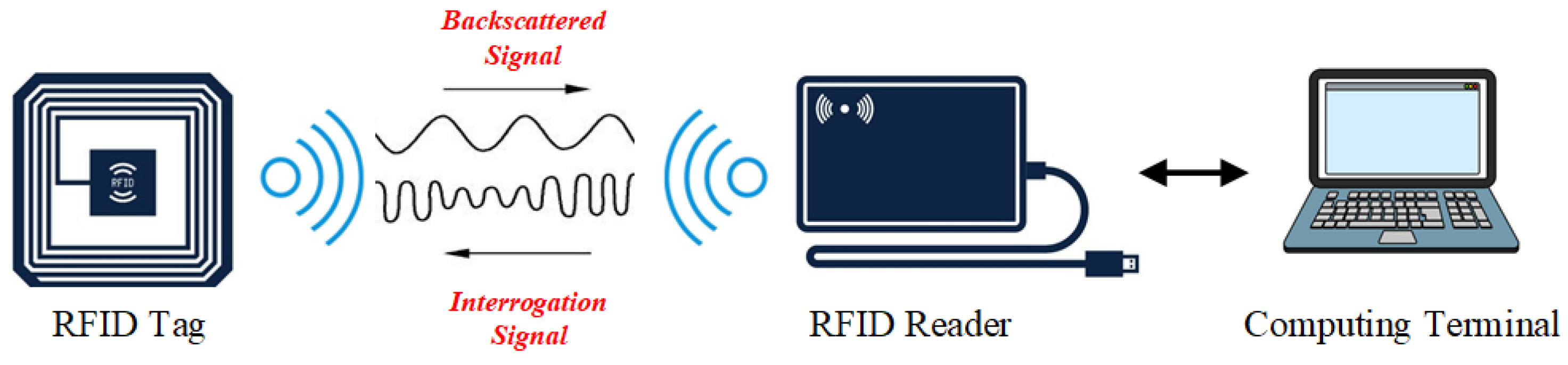
2.1. UHF RFID Communication Technology

Passive Ultra-High Frequency (UHF) RFID communication operates by utilizing radio waves in the UHF spectrum, typically between 856 MHz and 960 MHz, to enable the wireless transfer of data between a tag and a reader without the need for a battery within the tag.

In UHF RFID technology, the sensing mechanism involves two key processes: signal transmission from the tag chip to the reader and data exchange between the RFID reader and the processing computer. The interaction between the UHF RFID tag and the reader is based on backscatter modulation, where changes in the target object affect the backscattering signal characteristics. Figure 2 illustrates the transmission principle: the reader emits electromagnetic waves through its antenna, and, when an object with an RFID tag enters this field, the tag transmits its stored information back to the reader. The reader receives and processes this data, sending it to the main system via the I/O channel. The main system identifies the tag and executes control instructions for various internal processes.

When in an ideal experimental environment, based on free space, polarization matching, no loss, and port matching, the signal power received by the receiving the UHF RFID reader antenna $P_r$ is:

$$P_r={\displaystyle \frac{P_t{G}_r}{4\pi d^2}}·{\displaystyle \frac{G_t{\lambda }^2}{4\pi }}$$

(1)

where $P_t$ is the power emitted by the tag antenna, $G_t$ is the gain of the tag antenna, $G_r$ is the gain of the RFID reader antenna, $\lambda$ is the radio-frequency wavelength, and d is the distance between the antennas. When considering the addition of a medium between the tag and the reader, different media can affect the transmission of electromagnetic waves. In this context, we consider three indicators: RSSI, read/write distance, and phase. The following sections will provide a detailed explanation of each indicator.

• Read/Write Distance: Under ideal conditions, as indicated by (1), the received signal power at the antenna is directly influenced by the transmission distance. Considering real-world application scenarios, particularly in complex forest environments, the read/write distance cannot be considered a constant value. Therefore, it is essential to include read/write distance as a key indicator.
• RSSI: (1) represents the transmission under ideal conditions. When considering the insertion of a medium (in this study, leaves with different moisture content), we introduce a loss or gain factor $L_m$ caused by the presence of an object in the transmission path, as shown below:

  $$P_r^{\prime }={\displaystyle \frac{P_t{G}_r}{4\pi d^2}}·{\displaystyle \frac{G_t{\lambda }^2}{4\pi }}·L_m$$

  (2)

  where $P_r^{\prime }$ represents the received power at the antenna after accounting for the losses in the actual environment, $L_m$ represents the attenuation due to the object, which includes the penetration loss caused by the blocking or transmission of electromagnetic waves and the absorption loss due to the object. This type of loss is typically challenging to quantify in real-world environments. The backscattered signal strength RSSI through the tag represents the loss of the signal during the transmission process. The relationship between RSSI and signal power is as follows:

  $$\mathit{RSSI}=10·\lg ({\displaystyle \frac{P_r^{\prime }}{1\mathit{mW}}})$$

  (3)
• Phase: During the transmission process, due to the signal transmission characteristics of RFID, the total distance traveled by the radio-frequency signal during transmission is 2 d. The phase of the radio-frequency signal is also changing, which can be expressed as follows:

$$\varphi ={\displaystyle \frac{2\pi ·2d}{\lambda }}+{\varphi }_0$$

(4)

where ${\varphi }_0$ represents the initial phase. The actual phase value ${\varphi }^{\prime }$ output by the reader is as follows:

$${\varphi }^{\prime }=\varphi \mathit{mod}(2\pi )$$

(5)

When different media exist between the tag and the antenna, the dielectric constant of the medium affects the transmission of RF signals, and the impedance of the tag antenna changes, causing phase shifts. Therefore, we select the RSSI, RF phase, and measurement distance as indicators to invert the moisture content of the leaf.

In this paper, we exploit the unique properties of UHF RFID technology, which is sensitive to moisture and can penetrate non-metallic materials without direct contact and capture data from passive tags to read passive tags attached to the underside of leaves, capturing key data points, received signal strength indicators (RSSIs), phase, and read distance. By applying our proposed algorithm to analyze the collected data, we can accurately detect the moisture content of plant leaves. This approach offers a non-invasive, accurate, and efficient means of monitoring leaf moisture.

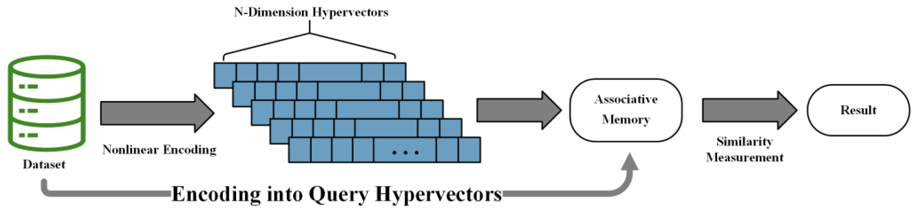
2.2. Hyperdimensional Computing

In a comprehensive evaluation of modern computing technologies, HDC demonstrates significant potential and application prospects through its rapid learning processes, low latency, high efficiency, robustness closely aligned with neuroscientific principles, compact model sizes, and reduced sample requirements. Figure 3 shows the basic block diagram of HDC. First, each real-valued feature in the dataset is encoded into a hyperdimensional vector of dimension N (usually N is thousands or tens of thousands) using a nonlinear coding method and then stored in the associative memory (AM) as a category hypervector after a series of operations (such as addition, multiplication, bundling, etc.). The hypervectors participating in the test form a query hypervector in the same encoding method, and then a series of similarity comparisons are performed in AM, and the result is output based on the difference in similarity. Below, we will introduce some basic theories of HDC, including its unique high-dimensional characteristics, calculation methods, some important indicators, etc.

2.2.1. Hyperdimensional Characteristics of HDC

In HDC, vectors are encoded into hypervectors of thousands, tens of thousands, or even higher dimensions. The incorporation of ultra-wide words inherently embeds redundancy, which shields against noise, thereby enhancing the system’s inherent robustness. In HDC, data representations within hypervectors predominantly fall into two categories: binary and non-binary. For binary vectors, the computational process is simplified, demanding lower computational power from hardware, which effectively leverages the advantages of HDC. On the other hand, non-binary vectors, typically utilizing integer or bipolar data formats, facilitate enhanced precision. Despite the incremental computational costs associated with non-binary representations, these are negligible when compared to the convolutional operations and gradient calculations prevalent in other artificial intelligence algorithms.

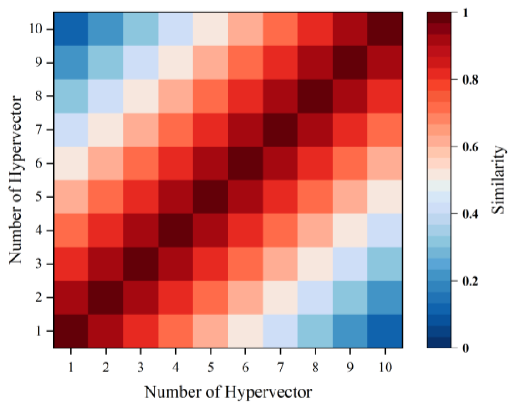
2.2.2. Similarity Criterion

For hypervectors encoded in different manners, various methods are employed to measure similarity. For binary hypervectors, the similarity between vectors is quantified using the Hamming distance, which is defined by (6):

$$\mathit{Ham}(A,B)={\displaystyle \frac{1}{d}}{\sum }_{i=1}^d{1}_{A\left(i\right)\ne B\left(i\right)}$$

(6)

where d represents the dimensionality of the hypervectors. It is evident from the above formula that the Hamming distance between two vectors increases with the number of differing elements at corresponding positions. Consequently, a larger Hamming distance indicates a lower similarity between the two hypervectors.

For hypervectors encoded in non-binary formats, the cosine distance method is utilized to measure their similarity:

$$c\mathrm{os}(A,B)={\displaystyle \frac{A·B}{\left|A\right|\left|B\right|}}$$

(7)

The cosine of the angle between two hypervectors is used as the criterion for determining their similarity. A cosine value closer to 1 indicates a higher degree of similarity between the vectors; conversely, when their angle is orthogonal, resulting in a cosine value of −1, it signifies that the vectors are completely opposite.

When the Hamming distance between two hypervectors is 0.5 or their cosine distance is 0, we consider the hypervectors to be orthogonal to each other. It is noteworthy that when the dimensionality of the hypervectors is sufficiently high (in the thousands or higher), two randomly selected hypervectors from the hyperdimensional space are highly likely to be orthogonal. Statistically, in a hyperdimensional space with 10,000 dimensions, the Hamming distance between a binary-encoded hypervector and any other randomly chosen hypervector has only a one in a million chance of being less than 0.476 or more than 0.524, and a one in a billion chance of being less than 0.470 or more than 0.530 [51]. This indicates that situations where the Hamming distance between two hypervectors is close to 1 or 0 are likely to occur only under artificial manipulation, a phenomenon known as the orthogonality in high dimensions.

2.2.3. Hyperdimensional Vector Operational Method

In HDC, operations on hypervectors involve three fundamental processes: addition, multiplication, and permutation. The following provides an introduction to these operations, illustrated with binary hypervectors as examples:

• Addition: Element-wise addition, also known as bundling operation, functions analogously to a majority vote mechanism. In this operation, when multiple hypervectors are added together, the element at each corresponding position in the newly generated hypervector is determined by the most frequently occurring element among all vectors at that position. The addition operation of three hypervectors using binary encoding is as follows:

$$\frac{\hfill \begin{array}{c}A=(0,0,0,0,1,0,0,1,1,1)\\ B=(1,0,1,1,0,0,0,1,0,1)\\ C=(0,0,1,0,1,0,1,1,0,1)\end{array}}{A+B+C=(0,0,1,0,1,0,0,1,0,1)}$$

(8)

• Multiplication: Element-wise multiplication, also referred to as binding, is primarily employed to establish an association between two hypervectors, such as binding a data value to its corresponding address. In the context of HDC, for hypervectors encoded in binary, element-wise multiplication is equivalent to the bitwise exclusive OR (XOR) operation, denoted by the symbol ⊕. When two vectors undergo multiplication, their corresponding elements are subjected to XOR, resulting in a new hypervector. In (9), we demonstrate the multiplication of two binary-coded hypervectors.

$$\frac{\hfill \begin{array}{c}A=(1,0,0,1,1,0,1,1)\\ B=(0,0,1,1,0,1,1,0)\end{array}}{A\oplus B=(1,0,1,0,1,1,0,1)}$$

(9)

• Permutation: In the realm of HDC, the permutation constitutes a distinctive computational procedure. This operation systematically reorganizes the elements of a hypervector through a predefined transformation schema. To capitalize on the hardware-compatibility benefits intrinsic to HDC, permutations are typically executed via cyclic shifting mechanisms, denoted by the symbol Π. The 8-dimensional binary hypervector A is arranged as follows:

$$\frac{\hfill A=(1,0,0,1,1,0,1,1)}{\mathsf{\Pi }A=(1,1,0,0,1,1,0,1)}$$

(10)

2.3. Encoding

In this section, we will detail the methodology for encoding features extracted from our collected data into hypervectors. In the data collection phase, data including RSSI, phase, and measurement distance were gathered by reading passive RFID tags attached to the back of tags. Utilizing the computational operations discussed above, a combination of different tag parameters is encoded into hypervectors.

We employed an address–data encoding method to process the collected data. For each data point, its corresponding address must remain independent and non-interfering. We randomly generated N hypervectors to serve as the addresses for each data vector. Due to the high-dimensional orthogonality of these hypervectors, they are mutually orthogonal, ensuring no interference during subsequent processing. For the values in each address, we adopt a method of continuous mapping for encoding. The encoding of L values within the range [Min, Max] into hyperdimensional vectors is as follows:

• Randomly generate a binary hypervector as the encoded minimum value, also referred to as the initial hypervector.
• Randomly flip d/2/(L−1) bits of the hypervector corresponding to the previous encoded value to encode the next hypervector, ensuring that each bit is flipped only once and not repeatedly.
• Repeat step 2 until all L values are encoded into hypervectors.

From the above steps, it is evident that upon completing the encoding of L data points, the difference between the first and last hypervectors precisely equals d/2 bits. Meanwhile, the intermediate hypervectors gradually diverge from the initial vector and increasingly approximate the last hypervector, enhancing their orthogonality progressively. The last encoded hypervector represents the maximum value of the dataset. After these operations, the address hypervector and value hypervector are bound through multiplication, forming a hyperdimensional vector for the address–value pair. Subsequently, after encoding all sample values and binding them through addition, we obtain the encoded representation of all samples for that feature.

For example, we encode ten levels of real-valued features in ascending order, where the minimum value corresponds to the hypervector of the first level, and the maximum value corresponds to the hypervector of the tenth level. Figure 4 illustrates the cosine similarity between hypervectors of different levels. It is evident that the greater the difference in real-valued features, the greater the cosine similarity between the encoded hypervectors.

In Figure 5, the data measured for the k-th label are assigned a hypervector $D_k$ randomly, with the ID serving as the address for the label. The measured value is encoded into a hypervector $V_k$ according to the aforementioned encoding method. R represents the result of binding the address hypervector and the value hypervector together for the corresponding data type.

$$R_{\mathit{Phase}}^1=D_1\times V_1$$

(11)

Γ represents the fusion of the three measured data types: phase, RSSI, and measured distance. The final hypervector representing the k-th sample is as follows:

$$C_1=\Gamma (R_{\mathit{Phase}}^1,R_{\mathit{Rssi}}^1,R_{\mathit{Dis}}^1)$$

(12)

We store these class hypervectors in the associative memory (AM). Subsequently, the test samples are encoded in the same manner as described above, and we refer to these as query hypervectors, denoted as Q_k, where k = 1, 2, 3, …, n, and n is the total number of query vectors. Then, for each class hypervector C and query hypervector Q, we calculate the cosine similarity. Finally, the query hypervector with the highest similarity is considered the result for the current sample.

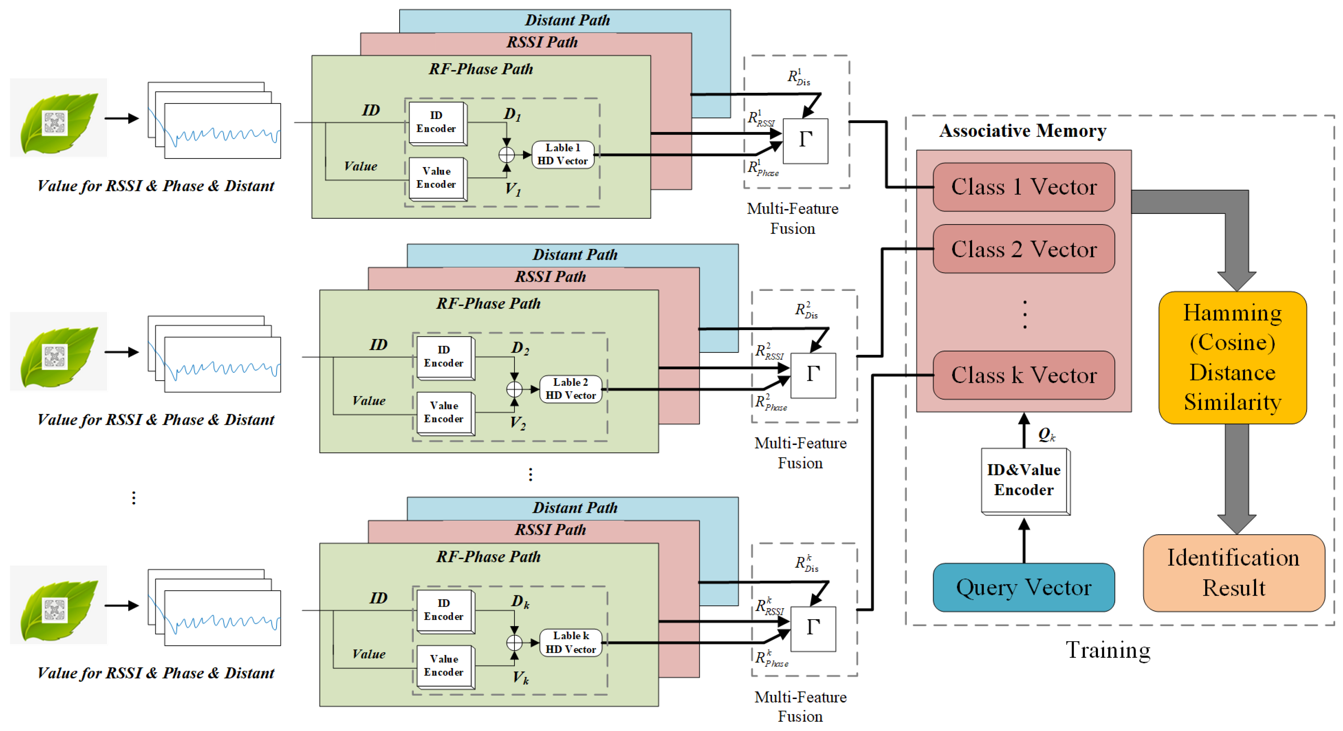
2.4. Multi-Feature Fusion

In preceding sections, we have delineated the application of addition or the bundling operation within the framework of HDC. Notably, this operation proves to be beneficial in scenarios involving samples with multiple attributes. For example, Naftali et al. [42] have successfully leveraged HDC to amalgamate multiple features of samples through addition operation on two distinct datasets related to diabetes, achieving notable accuracy in classification tasks. Nevertheless, the process of vector addition, wherein multiple hypervectors are aggregated bitwise, presents certain limitations. The post-addition process of binarizing the aggregated hypervector into a binary format ostensibly compromises the retention of critical information, potentially detracting from the efficacy of experiment results. Furthermore, this binarization approach introduces ambiguity in cases where an even number of hypervectors are aggregated, particularly when the frequencies of 0 s and 1 s are equivalent, rendering the value of the resultant bit as either 0 or 1 indeterminately.

We are committed to proposing a feature fusion algorithm to solve the above problems. The current mainstream feature fusion methods include Principal Component Analysis (PCA) [52], linear discriminant analysis (LDA) [53,54], etc. In our investigation, it has been observed that correlations exist among certain features of the samples, and a direct additive approach may result in the conflation of features. Consequently, this section is devoted to adapting the feature fusion technique, LDA, innovatively extending it to multi-dimensional feature fusion within our research framework. LDA operates on the principle of projecting features onto a linear axis. It articulates the concepts of between-class and within-class scatter, with the objective of minimizing the proximity of projection centers within the same category whilst maximizing the separation between those of distinct categories.

Given a dataset $D=\left\{\right(x_1,y_1),(x_2,y_2),\dots ,(x_m,y_m\left)\right\}$ comprising samples x_i as n-dimensional feature vectors with corresponding class vectors $y_i\in \{C_1,C_2,\dots ,C_k\}$, let N_j (j = 1, 2, …, k) denote the number of samples belonging to class j and X_j (j = 1, 2, …, k) represent the collection of samples for class j. The mean vector of the samples μ is calculated as follows:

$$\mu ={\displaystyle \frac{1}{n}}{\sum }_{j=1}^k{N}_j{\mu }_j$$

(13)

We define the within-class scatter matrix S_R as follows:

$$S_R=\sum _{j=1}^k{S}_{\mathit{rj}}=\sum _{j=1}^k\sum _{x\in X_j}(x-{\mu }_j\left)\right(x-{\mu }_j{)}^T$$

(14)

The total scatter matrix S_T is defined as follows:

$$S_T=\sum _{i=1}^n\left(x_i-\mu \right){\left(x_i-\mu \right)}^T=\sum _{j=1}^k\sum _{x\in X_j}(x-\mu \left)\right(x-\mu {)}^T$$

(15)

Hence, the between-class scatter matrix S_B is given by the following:

$$S_B=S_T-S_R=\sum _{j=1}^k{N}_j({\mu }_j-\mu ){\left({\mu }_j-\mu \right)}^T$$

(16)

For any sample x_i, its projection onto line r is given by r^Tx_i. Our objective is to minimize the within-class distance while maximizing the between-class distance, leading to the optimization of the following objective function:

$$\mathit{argmax}J\left(w\right)={\displaystyle \frac{{‖w^T{S}_{B}w‖}^2}{{‖w^T{S}_{R}w‖}^2}}=\prod _{i=1}^d{\displaystyle \frac{w_i^T{S}_B{w}_i}{w_i^T{S}_R{w}_i}}$$

(17)

Considering that the solution to the objective function is influenced solely by the direction of ω and not its magnitude, we can impose the constraint: w_i^Tw_i = 1.

Thus,

$$\left\{\begin{array}{c}\mathit{arg}\mathit{max}J(w)={\displaystyle \prod _{i=1}^d}{\displaystyle \frac{w_i^T{S}_B{w}_i}{w_i^T{S}_R{w}_i}}\\ s.t.w_i^T{w}_i=1\end{array}\right.$$

(18)

The problem can be solved by employing the method of Lagrange multipliers. Without delving into detailed operations, solving for the d generalized eigenvalues of the matrix S_R⁻¹S_B yields the hyperplane R as the matrix composed of corresponding eigenvectors. Therefore, the fused sample features can be represented as x_i^′ = w^Tx_i, ultimately achieving feature fusion. Figure 5 illustrates the implementation process of the algorithm, encompassing both the encoding and construction of hyperdimensional vectors, as well as the similarity measurement after the encoding is completed.

2.5. Re-Training

Due to the continuous addition and updating of training samples, it is inevitable that the misclassification of samples may occur. In [45], a retraining method was proposed by Imani et al. based on the following fundamental principle:

$$\left\{\begin{array}{c}{C^{\prime }}_{\mathrm{wrong}}=C_{\mathrm{wrong}}-\alpha Q_i\\ {C^{\prime }}_{\mathrm{correct}}=C_{\mathrm{correct}}+\alpha Q_i\end{array}\right.$$

(19)

In (19), Q_i represents the sample currently undergoing retraining, C is the original category matrix, and C^’ is the updated category matrix. By recalculating the similarity between the sample vector and category vectors, it determines the accuracy of classification. Incorrectly classified categories are then removed from their current category and reassigned to the correct one. Additionally, the article introduces, for the first time, the concept of a learning rate α from machine learning into HDC, proposing a method for the adaptive updating of α. Through iterative processes, the value of the learning rate α gradually decreases until convergence, with the learning rate controlling the extent of updates during each iteration of the model.

In the research conducted by Imani, the AdaptHD method stipulates the minimum value of α as 1, neglecting scenarios where α falls below 1. Additionally, in the pursuit of identifying the optimal value of α, there is a substantial risk of converging to a local optimum, which presents a challenge that necessitates resolution. To address this issue, we use an adaptive algorithm based on cosine annealing. Upon obtaining a minimum value, this algorithm aims to escape local minima by abruptly increasing the value of α, thereby facilitating the discovery of a path towards the global minimum. To solve the problem of getting stuck in local optima, we optimize the learning rate value based on the method of warm restarts. When the minimum value is reached, the learning rate is suddenly increased, and new parameters are determined based on those from the previous iteration cycle. The specific implementation method is as follows:

$${\eta }_t={\eta }_{\mathit{min}}^i+{\displaystyle \frac{1}{2}}\left({\eta }_{\mathit{max}}^i-{\eta }_{\mathit{min}}^i\right)\left(1+\mathit{cos}\left({\displaystyle \frac{T_{\mathit{cur}}}{T_i}}\pi \right)\right)$$

(20)

where η_t represents the current learning rate, η_min is the minimum learning rate, and η_max is the maximum learning rate, these two parameters delineate the range of the learning rate. T_cur denotes the current iteration number, and T_i signifies the total number of iterations.

Figure 6 presents the comprehensive flowchart of our LMC detection system. This diagram outlines the sequential steps and processes involved; first, using the established RFID system, we collected multiple sets of RSSI, phase, and reading distance data from the leaves. These real-valued features were then encoded into hyperdimensional vectors. Using the algorithm framework, we developed (as shown in Figure 5) and built an initial leaf moisture content (LMC) prediction model. The model was further optimized through a retraining process. Finally, the LMC results were predicted. Figure 6 (right side) illustrates the tuning process of the key parameter, α, during retraining.

3. Experiment Methodology

In this section, we discuss our experiments and results section in detail, including our experimental scenarios, equipment, dataset acquisition for the experiments, and analysis of the results. In our experiments, we used a computer device with a 13-th generation Intel Core i7 (14 cores, 4.90 GHz) (Intel, Santa Clara, CA, USA) and a memory of 16 GB. We conducted experiments in the Matlab 2022b environment. The model of the RFID reader was Impinj R420 UHF reader (Impinj, Seattle, WA, USA), the RYT-280 8.5dBi circular polarized antenna (UHF Internet of things Technology, Shenzhen, China) is used, and the tag is a square four-corner JT-IH47 waterproof RFID passive tag (Impinj in USA). The drying instrument used to measure the true moisture content of leaves is BEIYI-50A (Purify Science Instrument in Shanghai, China). Its weight accuracy is 0.001 g, and the maximum range is 50 g.

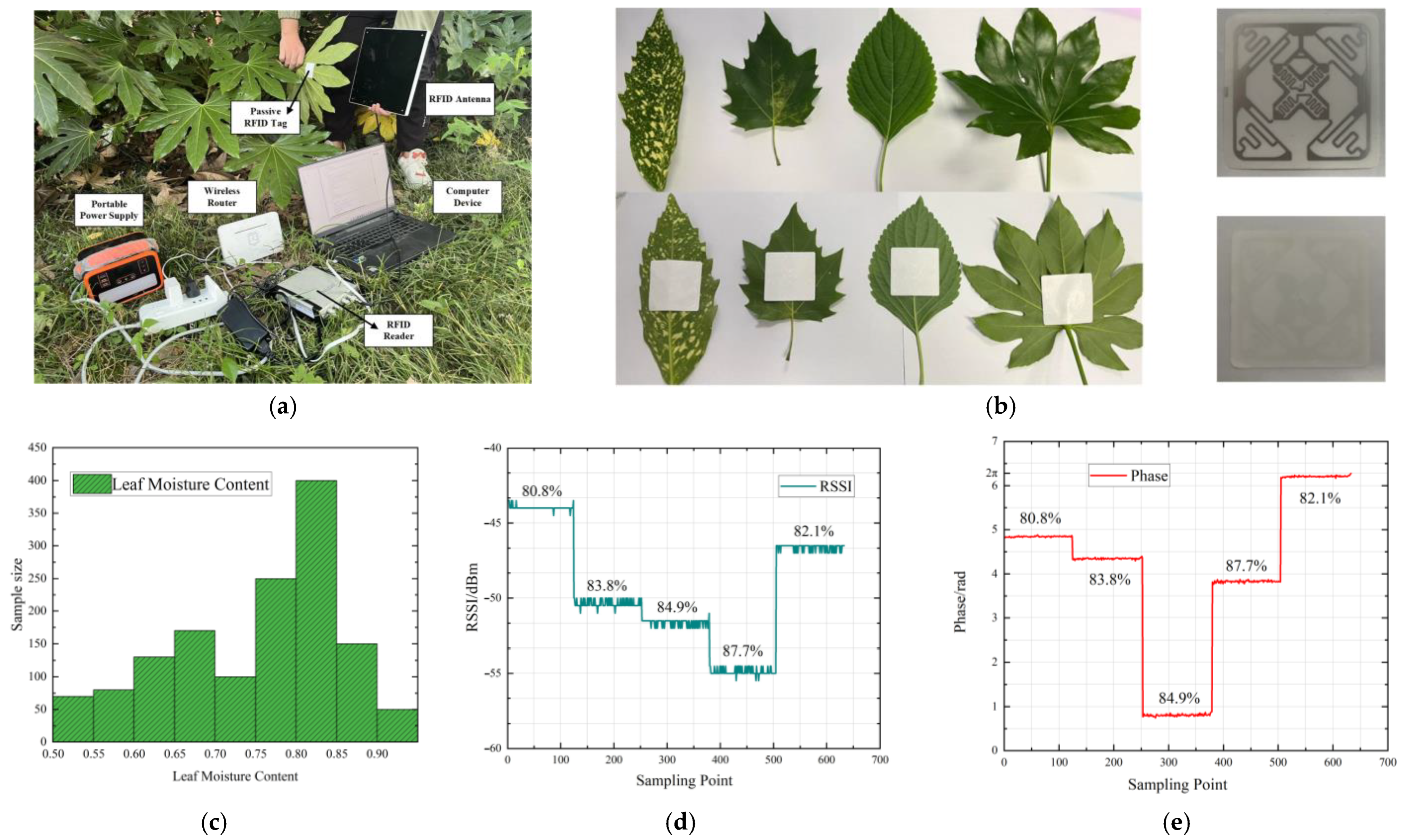
3.1. Leaf Moisture Data Acquisition

In our experimental methodology, we adopt a procedure that involves data collection followed by moisture content measurement, a common approach in the vast majority of plant moisture content detection studies. The data collection was conducted at the experimental forest of Nanjing Forestry University. We collected 1000 sets of valid data from the Experimental Forest Base of Nanjing Forestry University between February 2023 and February 2024, including leaf datasets under various moisture conditions such as fallen leaves, dead leaves, and living leaves. The leaves were harvested and immediately preserved in sealed bags to prevent water loss and then transported to the laboratory for measurement. As illustrated in Figure 7a, the sensor and the leaf were positioned securely to ensure that the RFID tag, attached to the back of the leaf, allows the radio-frequency signal to penetrate the leaf and reach the reader’s antenna. The antenna and the RFID tag were placed facing each other, parallel, with a wireless router serving to provide a local area network.

Figure 7 illustrates different aspects of our field measurement and experimental setup. Figure 7a shows the outdoor field measurement scenario. In Figure 7b, the left image depicts some of the leaf samples used in our experiments. The top part of this image shows the front sides of the leaves, while the bottom part displays the back sides along with the placement of the RFID tags. From left to right, the leaf samples include leaves of Aucuba japonica, Firmiana simplex, Perilla frutescens, and Fatsia japonica. The right image in Figure 7b displays the passive RFID tags used in the experiment. The top part shows the front side of the tags, which can be directly affixed to the surface of the object being measured, and the bottom part shows the back side of the tags.

Table 1. The name and the TSN of the experimental material.

Selected Materials	TSN
Fatsia japonica	505935
Aucuba japonica	565023
Perilla frutescens	32634
Firmiana simplex	21578

shows the names of the materials used in the experiment and their corresponding TSN (Taxonomic Serial Number).

The actual method for moisture content determination employed is the drying method, which involves heating the samples in a moisture drying oven at 110 °C for 3–4 h. After cooling, the samples are heated again until a constant weight is achieved (the difference between two consecutive weights is less than 0.1 g). The moisture content is then calculated using the following formula:

$$W={\displaystyle \frac{m_1-m_0}{m_0}}\times 100\%$$

(21)

where W represents the actual moisture content, m₁ is the initial mass of the leaf, and m₀ is the mass of the leaf after drying. Through the above methods, we collected 1000 sets of data at the experimental site for our research.

Table 2. Overview of the datasets measured during the experiment.

	Maximum	Minimum	Average	Standard Deviation
RSSI (dBm)	−24.0	−75.5	−44.05	5.857
Phase (rad)	6.277	0.006	3.149	2.022
Real Moisture Content (%)	91.28	47.65	80.29	7.138

shows the data we obtained during the study. Figure 7c shows the distribution of LMC. The leaves with a moisture content of 75% to 85% account for a large proportion. There are also a certain number of fallen leaves and dead leaves, whose moisture content is lower than the average level. In the experiment, we continuously measured the tags. Figure 7d,e show the RSSI and phase information of some leaves. Each sampling point represents each time the reader reads the tag.

3.2. Evaluation Metrics

To evaluate the performance of our moisture content detection, we utilize three key metrics: RMSE (Root Mean Square Error), MAE (Mean Absolute Error), and the Coefficient of Determination, denoted as R². RMSE provides a measure of the magnitude of the error by calculating the square root of the average squared differences between the predicted values and the actual values. RMSE is particularly useful because it penalizes larger errors more severely, providing a clear indication of larger discrepancies in prediction. MAE measures the average magnitude of the errors in a set of predictions, without considering their direction. It is the average over the test sample of the absolute differences between prediction and actual observation where all individual differences have equal weight. The formulas of the above three evaluation indicators are as follows:

$$\mathit{MAE}={\displaystyle \frac{1}{m}}{\displaystyle \sum _{i=1}^m\left|h(x_i)-y_i\right|}$$

(22)

$$\mathit{RMSE}(X,h)=\sqrt{{\displaystyle \frac{1}{m}}{\displaystyle \sum _{i=1}^m{\left(h(x_i)-y_i\right)}^2}}$$

(23)

where h(x_i) represents the actual value of the i-th group of data, y_i represents the predicted value in the i-th group of data.

R² provides an indication of the goodness of fit of the predictions. It is a proportion that explains how much of the variability in the outcome can be explained by the model’s inputs. The R² of 1 indicates that the regression predictions perfectly fit the data, while an R² of 0 indicates that the model explains none of the variability of the response data around its mean.

$$R^2={\displaystyle \frac{{\displaystyle \sum _{i=1}^n{\left({\widehat{y}}_i-\overline{y}\right)}^2}}{{\displaystyle \sum _{i=1}^n{\left(y_i-\overline{y}\right)}^2}}}=1-{\displaystyle \frac{{\displaystyle \sum _{i=1}^n{\left(y_i-\widehat{y}\right)}^2}}{{\displaystyle \sum _{i=1}^n{\left(y_i-\overline{y}\right)}^2}}}$$

(24)

where y are the data to be fitted, the mean of y is ӯ, and the fitted data are ŷ.

4. Result and Discussion

In this section, we will apply the algorithm we developed to the dataset we have collected. Initially, we will evaluate the model’s accuracy before and after feature fusion. Subsequently, we will discuss and assess the retraining method proposed. Finally, we will compare our model against several contemporary machine (deep) learning algorithms.

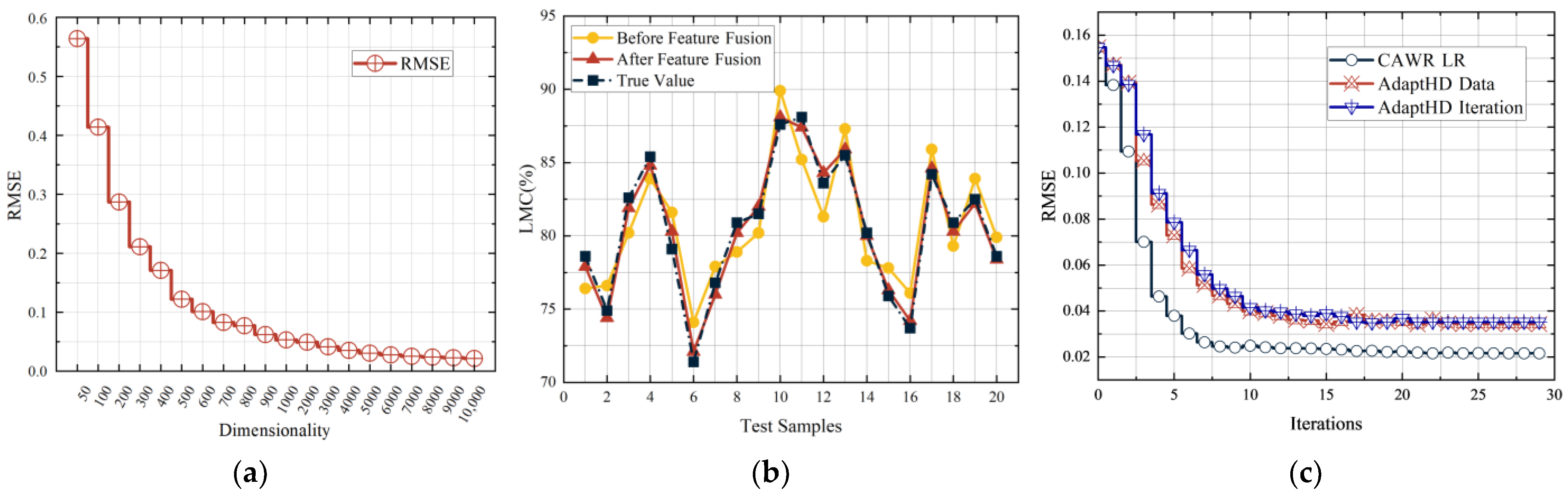
4.1. Paramaters Determined

In HDC, the dimensionality of the hypervectors is a crucial parameter as it directly influences the computational load, encoding complexity, and ultimately the performance of the model. We experimented with dimensions ranging from 50 to 10,000 to determine the most suitable dimensionality for our needs. The results, as shown in Figure 8a, indicate that at very low dimensions, the model exhibits substantial errors. However, as the dimensionality increases, the accuracy of the model progressively improves. Consequently, we opted for a dimensionality of 10,000 for our experiments, which also confirmed the previously mentioned orthogonality properties of hypervectors at higher dimensions.

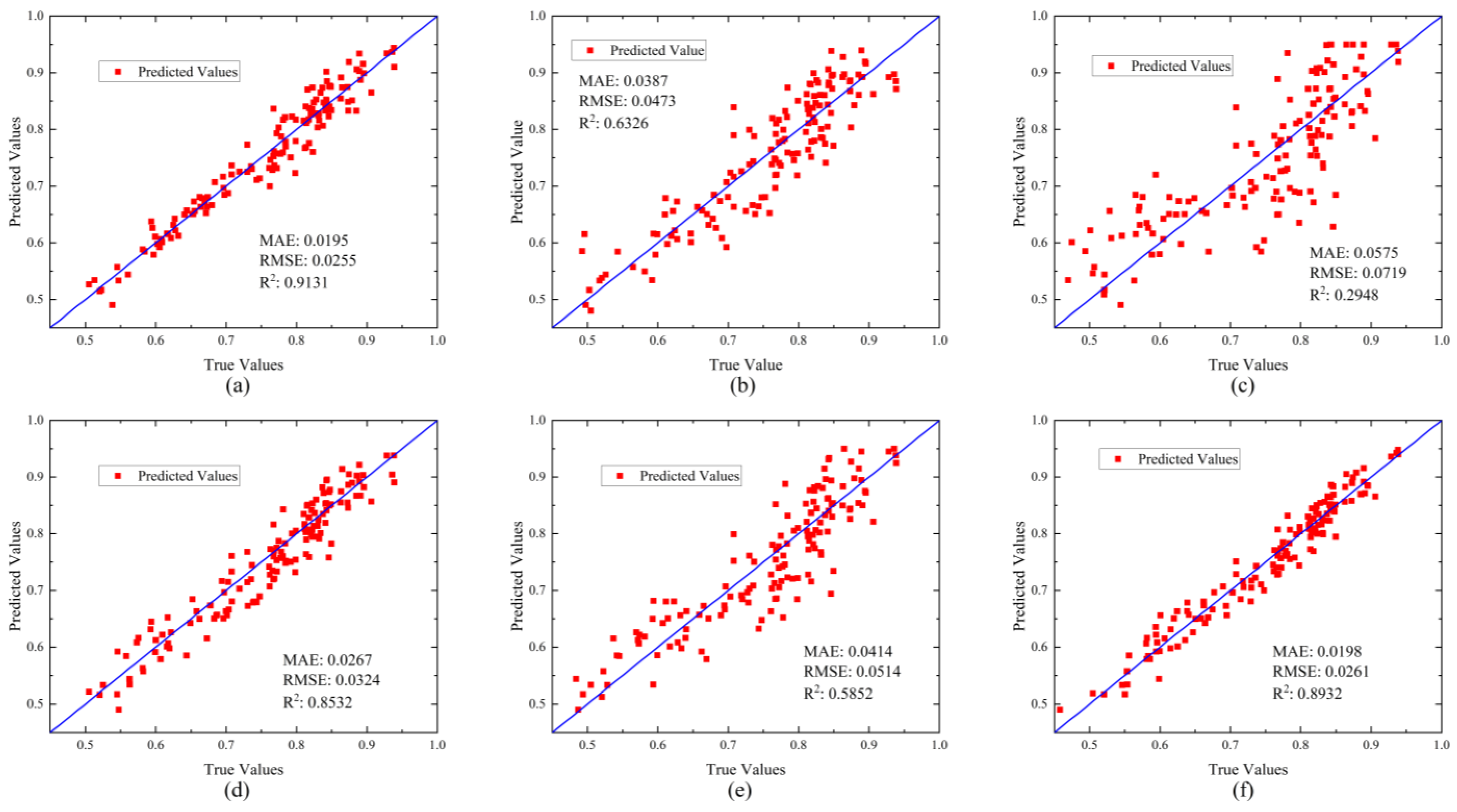
4.2. Experimental Comparison before and after Multi-Feature Fusion

Due to the multifaceted nature of the data collected, which comprises several interrelated features, there is a potential risk of decreased detection accuracy due to feature overlap. In Section 2.4, we introduced the application of LDA within the framework of HDC. In this section, we train the HDC network using the data samples collected before and after feature fusion and subsequently test the model on a test dataset. The dimensionality of the HDC is set to 10,000, the training set, test set, and validation set are divided into 7:2:1. The detection results, pre and post feature fusion, are illustrated in the following Figure 8b. The results indicate a significant improvement in experimental outcomes following feature fusion.

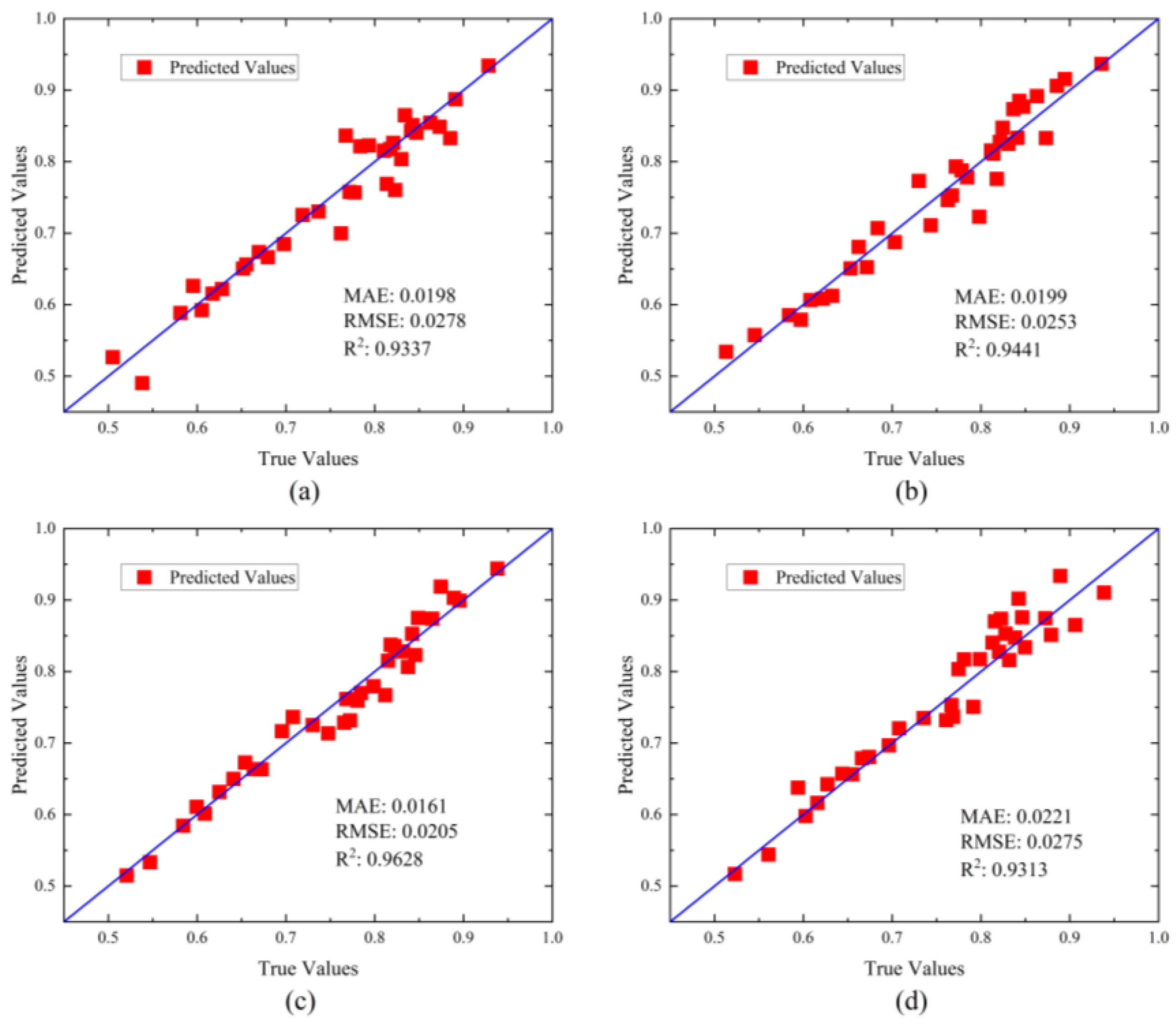
4.3. Re-Training Methods

In traditional HDC algorithms, real-valued features are encoded once and then directly input into the algorithm for similarity comparison, which can lead to decreased accuracy due to misclassification of some hypervectors. To address this issue, we propose a retraining method, inspired by simulated cosine annealing. This method introduces the learning rate α and continuously optimizes its value to refine the model. Compared to the classical AdaptHD approach, our method extends the consideration of learning rates below 1 and effectively resolves the problem of becoming trapped in local optima.

In AdaptHD [45], retraining is divided into two approaches: an iteration-based method and a data-based method. We conducted experiments within a 10,000-dimensional hyperdimensional space using both methods of AdaptHD as well as our proposed method. The results of these experiments are illustrated in Figure 8c below. The results indicate that after multiple iterations, all three methods converge to an optimal solution. Compared to each individual method within AdaptHD, our proposed retraining approach demonstrates superior performance in terms of both the convergence speed and the accuracy of the model.

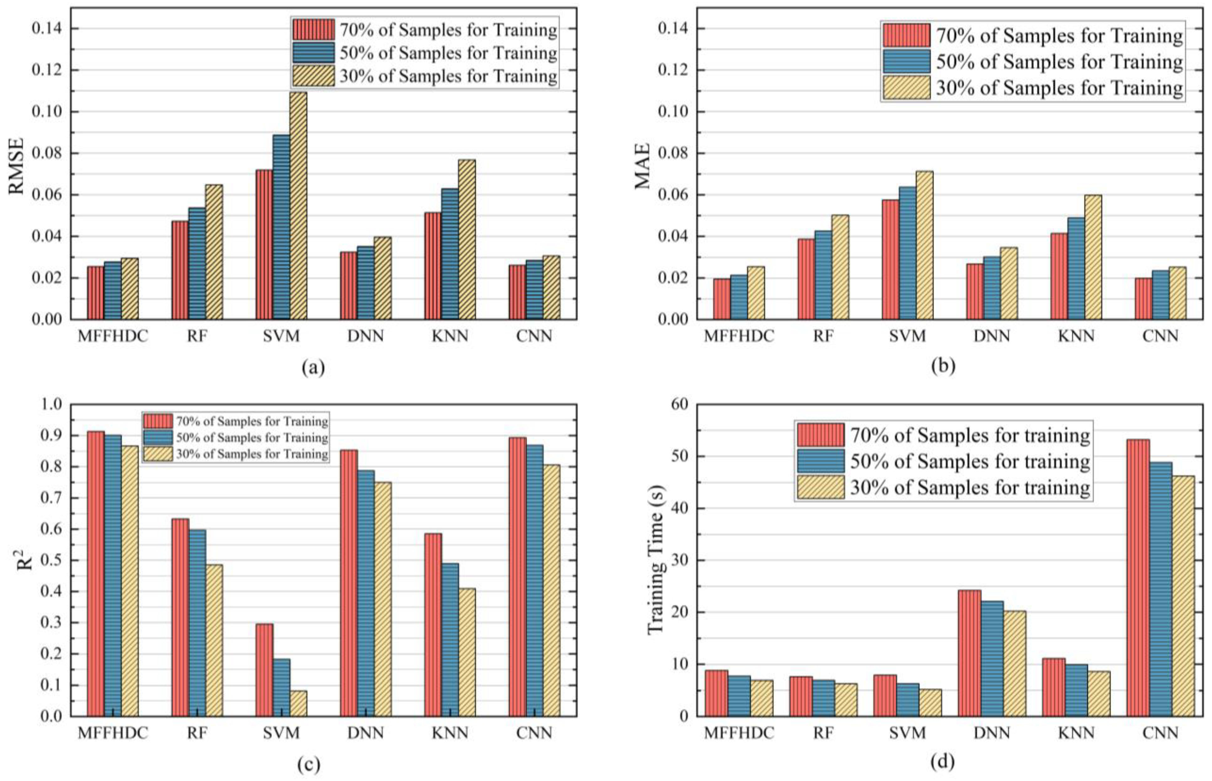
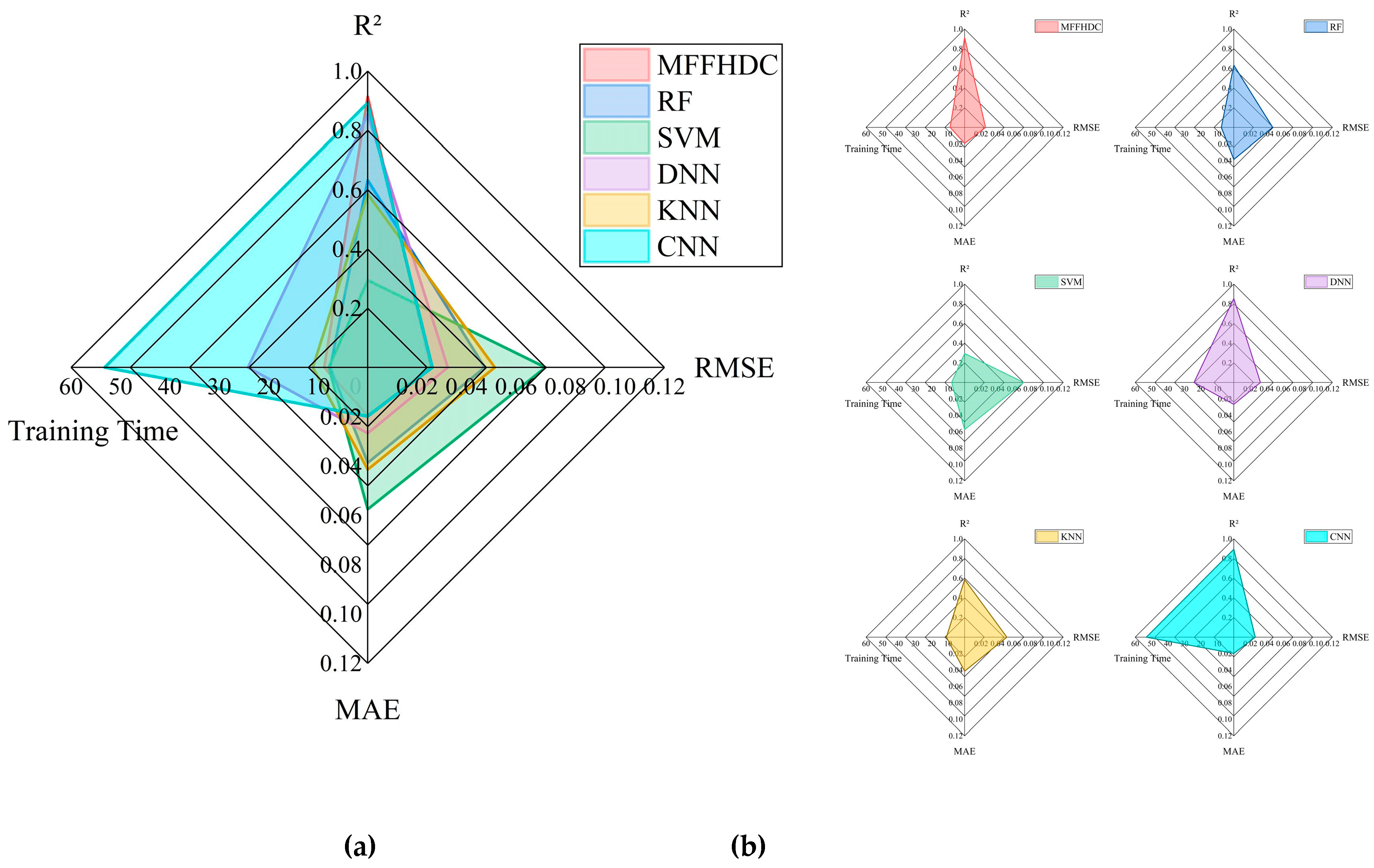
4.4. Performance Evaluation

In this section, we conduct a comparative evaluation of our proposed HDC-based method against several widely used machine (deep) learning algorithms—namely, Random Forest (RF), Support Vector Machine (SVM), Deep Neural Network (DNN), K-Nearest Neighbors (KNN), and Convolutional Neural Network (CNN). The evaluation focuses on metrics including MAE, RMSE, R², and training time. The detailed descriptions are listed in

Table 3. Algorithms used in contrast experiment.

Algorithm Name	Details
MFFHDC	The dimensional of hypervector is 10,000.
Random Forest	The n_estimators is 100, the max_depth is 30, the min_samples_split is 2, and the min_samples_leaf is 1.
Support Vector Machine	The type of kernel function is linear kernel function, and the value of C parameter is 100.
KNN	The number of neighbors is set to 10, the algorithm is set to auto, and the weights select distance.
DNN	There are two fully connected layers, the number of neurons in each layer is 64, the activation function is ReLU, and the loss function is MSE.
CNN	There are 2 convolution layers, 32 convolution kernels, 2 pooling layers, and 2 fully connected layers. The activation function is ReLU, and MSE is the loss function.

.

The parameters of our MFFHDC model were set to 10,000 dimensions. To enhance the credibility of our results, we conducted experiments with varying training-set ratios of 70%, 50%, and 30% within the dataset, and the results are displayed in Figure 9. In terms of experimental error, traditional simple machine learning algorithms such as Random Forest and SVM underperformed. With training-set ratios of 70%, 50%, and 30%, the RMSE values of our proposed MFFHDC method were 0.0255, 0.0276, and 0.0322, respectively, and the MAE values were 0.0195, 0.0224, and 0.0278, respectively. These accuracy metrics significantly surpassed those of Random Forest, SVM, and KNN. Moreover, the computational cost of HDC was much lower than that of CNN, making it a more efficient alternative.

In terms of the R² coefficient, a measure of the proportion of variance for a dependent variable that is explained by an independent variable or variables in a regression model, our proposed HDC model also exhibited strong performance. With training-set ratios of 70%, 50%, and 30%, the HDC model achieved R² values of 0.9131, 0.8966, and 0.8465, respectively, placing it in a favorable position compared to competing models. Regarding training times, with training set proportions of 70%, 50%, and 30%, our proposed HDC model required only 8.8 s, 7.6 s, and 6.8 s, respectively. It is clear that HDC’s training duration is significantly shorter than that required by some deep learning models, such as DNN and CNN, especially considering that the difference in model accuracy is minimal. For instance, at a training-set proportion of 70%, the training time for HDC was 2.75 times faster than DNN and 6.05 times faster than CNN. Compared to KNN, HDC’s training time was also 1.26 times quicker. This efficiency in training time, coupled with competitive accuracy, highlights HDC’s potential as an effective alternative to more computationally demanding models.

Table 4. Performances of different machine (learning) algorithms.

Algorithm Model	MAE	RMSE	R2	Training Time
MFFHDC	0.0195	0.0255	0.9131	8.8
RF	0.0387	0.0473	0.6326	7.6
SVM	0.0575	0.0719	0.2948	7.9
DNN	0.0267	0.0324	0.8532	24.2
KNN	0.0414	0.0514	0.5852	11.1
CNN	0.0198	0.0261	0.8932	53.2

shows the experimental results in the form of tabular data.

We set the ratio of training set, test set, and validation set to 7:2:1 and compared several algorithms in terms of RMSE, MAE, R², and training time. Figure 10; Figure 11 show the experimental results. Under the comprehensive evaluation indicators, our proposed methods all have excellent performance.

Different types of leaves exhibit variations in certain features, such as leaf thickness and leaf density. To verify the reliability of the LMC detection system proposed in this paper, we classified the collected leaf samples into different categories and conducted separate experiments on each category. The experimental results are shown in Figure 12. The system has good prediction results when facing different types of leaves, proving that the prediction model has strong generalization ability and good robustness.

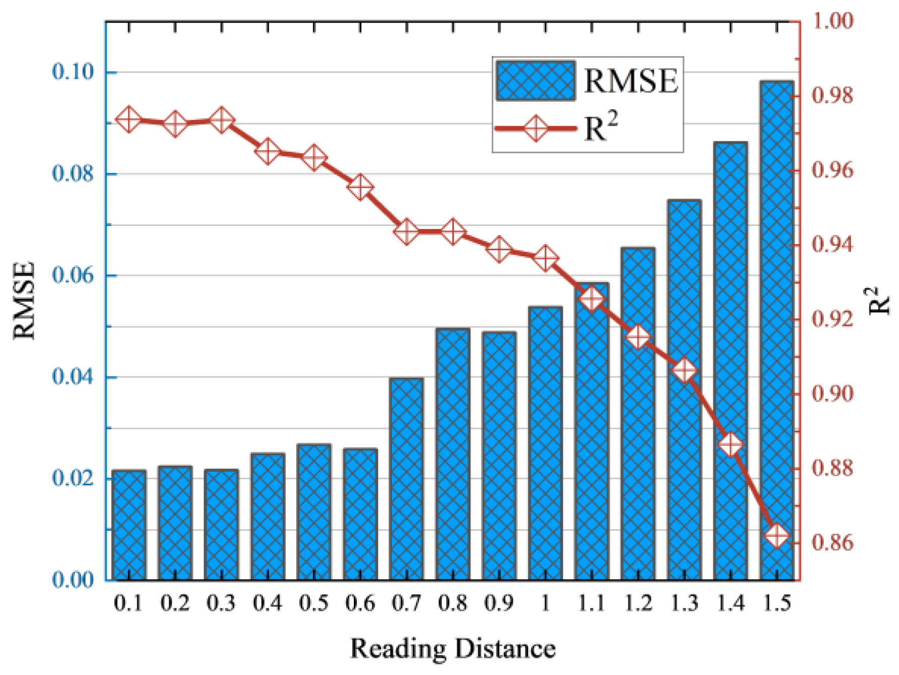
4.5. Farthest Distance Threshold Test

Considering practical applications, we assessed the performance of our model at different distances between the tags and the reader. As illustrated in Figure 13, when the distance between the reader and the tag was 1 m, the RMSE remained low at 0.0538, and the R² was quite strong at 0.9365.

The model exhibited solid performance when the reading distance of the reader was 1 m or less. It is worth noting that environmental factors, such as increased electromagnetic interference from external sources, tend to increase as the distance between the reader and the tag increases. Nonetheless, the results demonstrate that our system performs well in real-world settings.

5. Conclusions

In this paper, we propose a novel LMC detection model based on the UHF RFID and HDC algorithm. First, data such as RSSI, phase, and reading distance were collected using an RFID reader from passive tags attached to the back of the leaves. After data collection, the leaves were immediately harvested, sealed, and transported to the laboratory for drying and precise moisture content measurement. In the proposed HDC algorithm, real-world features were first encoded into hypervectors through linear mapping. To address feature overlap in feature interactions, we introduced a feature fusion method. Finally, to improve detection accuracy, we implemented a retraining method based on cosine annealing. The final model achieved MAE, RMSE, and R² values of 0.0195, 0.0255, and 0.9131, respectively.

This study has validated the initial hypotheses proposed in the introduction through experiments and data analysis. Specifically, (1) different moisture contents caused significant changes in the dielectric constant of the leaves. By analyzing the dielectric properties of the leaves using the proposed MFF-HDC algorithm, we successfully inferred the leaf moisture content, and the results demonstrated that this method has high accuracy and reliability. (2) The experimental results showed that UHF radio-frequency signals are highly sensitive to changes in leaf moisture content. By measuring the phase, RSSI, and reading distance of the signals through the UHF RFID system, we successfully quantified the dielectric properties under different moisture content conditions, further supporting our hypothesis. (3) We demonstrated that our method performed well across different types of leaves, and other characteristics such as salinity and chlorophyll had little to no impact on the results.

In summary, the experimental results support our initial hypotheses and validate the feasibility of predicting leaf moisture content using UHF RFID and HDC.

Since this is the first application of our method to measure LMC, we recognize several temporary issues and propose the following directions for future improvement:

• Noise from environmental factors and the RFID reader can reduce detection accuracy. Future research should develop advanced noise filtering and signal processing algorithms to improve precision.
• Inconsistent alignment between tags and the reader in forest environments affects accuracy. Flexible mounting mechanisms or enhanced antenna systems can mitigate this. To further solve this problem, our next research focus will be on the design of the internal structure of the RFID tag suitable for most LMC detection. We believe that field effect transistors [55] are a good choice for applying them to label design, and we will continue to explore other possible methods to achieve further results in our research.
• Future studies could expand to measure moisture content across entire trees or plant areas, using multi-sensor data fusion for a comprehensive understanding of vegetation moisture and plant health.

We plan to addressing these issues and conducting further in-depth research to improve the accuracy and application scope of LMC detection. This will provide more reliable technical support for vegetation health monitoring.

References

1. Du, Y.L.; Zhao, Q.; Chen, L.R.; Yao, X.D.; Zhang, W.; Zhang, B.; Xie, F.T. Effect of drought stress on sugar metabolism in leaves and roots of soybean seedlings. Plant Physiol. Biochem. 2020, 146, 1–12. [Google Scholar] [CrossRef] [PubMed]
2. Ramzan, R.; Omar, M.; Siddiqui, O.F.; Ksiksi, T.S.; Bastaki, N. Internet of Trees (IoTr) Implemented by Highly Dispersive Electromagnetic Sensors. IEEE Sens. J. 2021, 21, 642–650. [Google Scholar] [CrossRef]
3. Babu, A.K.; Kumaresan, G.; Raj, V.A.A.; Velraj, R. Review of leaf drying: Mechanism and influencing parameters, drying methods, nutrient preservation, and mathematical models. Renew. Sustain. Energy Rev. 2018, 90, 536–556. [Google Scholar] [CrossRef]
4. Shen, S.; Hua, J.J.; Zhu, H.K.; Yang, Y.Q.; Deng, Y.L.; Li, J.; Yuan, H.B.; Wang, J.J.; Zhu, J.Y.; Jiang, Y.W. Rapid and real-time detection of moisture in black tea during withering using micro-near-infrared spectroscopy. LWT-Food Sci. Technol. 2022, 155, 9. [Google Scholar] [CrossRef]
5. Dong, C.W.; An, T.; Yang, M.; Yang, C.S.; Liu, Z.Y.; Li, Y.; Duan, D.D.; Fan, S.X. Quantitative prediction and visual detection of the moisture content of withering leaves in black tea (Camellia sinensis) with hyperspectral image. Infrared Phys. Technol. 2022, 123, 104118. [Google Scholar] [CrossRef]
6. An, T.; Yu, S.Y.; Huang, W.Q.; Li, G.L.; Tian, X.; Fan, S.X.; Dong, C.W.; Zhao, C.J. Robustness and accuracy evaluation of moisture prediction model for black tea withering process using hyperspectral imaging. Spectrochim. Acta Part A-Mol. Biomol. Spectrosc. 2022, 269, 120791. [Google Scholar] [CrossRef]
7. Wei, Y.Z.; Wu, F.Y.; Xu, J.; Sha, J.J.; Zhao, Z.F.; He, Y.; Li, X.L. Visual detection of the moisture content of tea leaves with hyperspectral imaging technology. J. Food Eng. 2019, 248, 89–96. [Google Scholar] [CrossRef]
8. Sun, J.; Zhou, X.; Hu, Y.G.; Wu, X.H.; Zhang, X.D.; Wang, P. Visualizing distribution of moisture content in tea leaves using optimization algorithms and NIR hyperspectral imaging. Comput. Electron. Agric. 2019, 160, 153–159. [Google Scholar] [CrossRef]
9. Liu, Y.; Zhou, X.; Sun, J.; Li, B.; Ji, J.Y. A Method for Non-destructive Detection of Moisture Content in Oilseed Rape Leaves Using Hyperspectral Imaging Technology. J. Nondestruct. Eval. 2024, 43, 32. [Google Scholar] [CrossRef]
10. Li, B.; Zhao, X.T.; Zhang, Y.; Zhang, S.J.; Luo, B. Prediction and monitoring of leaf water content in soybean plants using terahertz time-domain spectroscopy. Comput. Electron. Agric. 2020, 170, 105239. [Google Scholar] [CrossRef]
11. Othman, Y.; Steele, C.; VanLeeuwen, D.; Heerema, R.; Bawazir, S.; St Hilaire, R. Remote sensing used to detect moisture status of pecan orchards grown in a desert environment. Int. J. Remote Sens. 2014, 35, 949–966. [Google Scholar] [CrossRef]
12. Steele-Dunne, S.C.; Friesen, J.; van de Giesen, N. Using Diurnal Variation in Backscatter to Detect Vegetation Water Stress. IEEE Trans. Geosci. Remote Sens. 2012, 50, 2618–2629. [Google Scholar] [CrossRef]
13. Basyigit, I.B. The examination and modeling of moisture content effect of banana leaves on dielectric constant for remote sensing. Microw. Opt. Technol. Lett. 2020, 62, 1087–1092. [Google Scholar] [CrossRef]
14. Tang, L.; Gao, S.D.; Wang, W.; Xiong, X.F.; Han, W.T.; Li, X.S. Moisture Content Detection of Tomato Leaves Based on Electrical Impedance Spectroscopy. Commun. Soil Sci. Plant Anal. 2024, 55, 609–623. [Google Scholar] [CrossRef]
15. Jabbar, A.; Omar, M.; Ramzan, R.; Siddiqui, O.F. Internet of Trees (IoTr): A Low-Cost Single Stub Lorentz Resonator For Plant Moisture Sensing. In Proceedings of the 18th International Bhurban Conference on Applied Sciences and Technologies (IBCAST), Islamabad, Pakistan, 12–16 January 2021; pp. 979–982. [Google Scholar] [CrossRef]
16. Han, W.T.; Yu, S.; Xu, T.F.; Chen, X.W.; Ooi, S.K. Detecting maize leaf water status by using digital RGB images. Int. J. Agric. Biol. Eng. 2014, 7, 45–53. [Google Scholar] [CrossRef]
17. Yang, Z.Y.; He, W.Y.; Fan, X.J.; Tjahjadi, T. PlantNet: Transfer learning-based fine-grained network for high-throughput plants recognition. Soft Comput. 2022, 26, 10581–10590. [Google Scholar] [CrossRef]
18. Zhu, Y.X.; Sun, W.M.; Cao, X.Y.; Wang, C.Y.; Wu, D.Y.; Yang, Y.; Ye, N. TA-CNN: Two-way attention models in deep convolutional neural network for plant recognition. Neurocomputing 2019, 365, 191–200. [Google Scholar] [CrossRef]
19. Rong, Q.J.; Hu, C.H.; Hu, X.D.; Xu, M.X. Picking point recognition for ripe tomatoes using semantic segmentation and morphological processing. Comput. Electron. Agric. 2023, 210, 107923. [Google Scholar] [CrossRef]
20. Yu, Y.F.; Fu, L.Y.; Cheng, Y.W.; Ye, Q.L. Multi-view distance metric learning via independent and shared feature subspace with applications to face and forest fire recognition, and remote sensing classification. Knowl.-Based Syst. 2022, 243, 108350. [Google Scholar] [CrossRef]
21. Lin, H.F.; Liu, X.Y.; Wang, X.Y.; Liu, Y.F. A fuzzy inference and big data analysis algorithm for the prediction of forest fire based on rechargeable wireless sensor networks. Sustain. Comput.-Inform. Syst. 2018, 18, 101–111. [Google Scholar] [CrossRef]
22. Cheng, Y.W.; Fu, L.Y.; Luo, P.; Ye, Q.L.; Liu, F.; Zhu, W. Multi-view generalized support vector machine via mining the inherent relationship between views with applications to face and fire smoke recognition. Knowl.-Based Syst. 2020, 210, 106488. [Google Scholar] [CrossRef]
23. Fan, X.J.; Luo, P.; Mu, Y.; Zhou, R.; Tjahjadi, T.; Ren, Y. Leaf image based plant disease identification using transfer learning and feature fusion. Comput. Electron. Agric. 2022, 196, 106892. [Google Scholar] [CrossRef]
24. Shivling, V.D.; Singh, A.; Bansod, B.K.; Nag, U.; Meena, D.L. Feasibility study of patch antenna for monitoring moisture content of made tea. J. Microw. Power Electromagn. Energy 2022, 56, 192–200. [Google Scholar] [CrossRef]
25. Colak, B. Moisture content effect of banana leaves to radio frequency absorbing. Microw. Opt. Technol. Lett. 2019, 61, 2591–2595. [Google Scholar] [CrossRef]
26. Tein, S.Y.; Then, Y.L.; You, K.Y. Tea Leaves Moisture Measurement and Prediction Using RF Waveguide Antenna. In Proceedings of the 2017 IEEE Asia Pacific Microwave Conference (APMC), Kuala Lumpur, Malaysia, 13–16 November 2017; pp. 670–673. [Google Scholar] [CrossRef]
27. Peng, B.; Liu, X.X.; Yao, Y.; Ping, J.F.; Ying, Y.B. A wearable and capacitive sensor for leaf moisture status monitoring. Biosens. Bioelectron. 2024, 245, 115804. [Google Scholar] [CrossRef]
28. Colella, R.; Catarinucci, L.; Grassi, G. Battery-less RF-powered circuits for non-contact voltage monitoring of electric systems: Circuit modeling and SPICE analysis. Int. J. Circuit Theory Appl. 2024. (Early Access). [Google Scholar] [CrossRef]
29. Daskalakis, S.N.; Assimonis, S.D.; Goussetis, G.; Tentzeris, M.M.; Georgiadis, A. The Future of Backscatter in Precision Agriculture. In Proceedings of the USNC-URSI Radio Science Meeting/IEEE International Symposium on Antennas and Propagation (AP-S), Atlanta, GA, USA, 7–12 July 2019; IEEE: Piscataway, NJ, USA, 2019; pp. 647–648. [Google Scholar]
30. Costa, F.; Genovesi, S.; Borgese, M.; Michel, A.; Dicandia, F.A.; Manara, G. A Review of RFID Sensors, the New Frontier of Internet of Things. Sensors 2021, 21, 3138. [Google Scholar] [CrossRef]
31. Daskalakis, S.N.; Goussetis, G.; Assimonis, S.D.; Tentzeris, M.M.; Georgiadis, A. A uW Backscatter-Morse-Leaf Sensor for Low-Power Agricultural Wireless Sensor Networks. IEEE Sens. J. 2018, 18, 7889–7898. [Google Scholar] [CrossRef]
32. Melià-Segní, J.; Vilajosana, X. Ubiquitous moisture sensing in automaker industry based on standard UHF RFID tags. In Proceedings of the IEEE International Conference on RFID (IEEE RFID), Phoenix, AZ, USA, 2–4 April 2019; IEEE: Piscataway, NJ, USA, 2019. [Google Scholar] [CrossRef]
33. Wu, Y.; Zhang, C.W.; Liu, W.B. Living Tree Moisture Content Detection Method Based on Intelligent UHF RFID Sensors and OS-PELM. Sensors 2022, 22, 6287. [Google Scholar] [CrossRef]
34. Thomas, A.; Dasgupta, S.; Rosing, T. A Theoretical Perspective on Hyperdimensional Computing. J. Artif. Intell. Res. 2021, 72, 215–249. [Google Scholar] [CrossRef]
35. Kanerva, P. Hyperdimensional Computing: An Introduction to Computing in Distributed Representation with High-Dimensional Random Vectors. Cogn. Comput. 2009, 1, 139–159. [Google Scholar] [CrossRef]
36. Imani, M.; Kong, D.Q.; Rahimi, A.; Rosing, T. VoiceHD: Hyperdimensional Computing for Efficient Speech Recognition. In Proceedings of the IEEE International Conference on Rebooting Computing (ICRC), Washington, DC, USA, 8–9 November 2017; IEEE: Piscataway, NJ, USA, 2017; pp. 97–104. [Google Scholar] [CrossRef]
37. Imani, M.; Hwang, J.; Rosing, T.; Rahimi, A.; Rabaey, J.M. Low-Power Sparse Hyperdimensional Encoder for Language Recognition. IEEE Des. Test 2017, 34, 94–101. [Google Scholar] [CrossRef]
38. Li, H.T.; Wu, T.F.; Rahimi, A.; Li, K.S.; Rusch, M.; Lin, C.H.; Hsu, J.L.; Sabry, M.M.; Eryilmaz, S.B.; Sohn, J.; et al. Hyperdimensional Computing with 3D VRRAM In-Memory Kernels: Device-Architecture Co-Design for Energy-Efficient, Error-Resilient Language Recognition. In Proceedings of the 62nd Annual IEEE International Electron Devices Meeting (IEDM), San Francisco, CA, USA, 3–7 December 2016. [Google Scholar] [CrossRef]
39. Chang, E.J.; Rahimi, A.; Benini, L.; Wu, A.Y. Hyperdimensional Computing-based Multimodality Emotion Recognition with Physiological Signals. In Proceedings of the 1st IEEE International Conference on Artificial Intelligence Circuits and Systems (AICAS), Hsinchu, Taiwan, 18–20 March 2019; IEEE: Piscataway, NJ, USA, 2019; pp. 137–141. [Google Scholar] [CrossRef]
40. Rahimi, A.; Kanerva, P.; Benini, L.; Rabaey, J.M. Efficient Biosignal Processing Using Hyperdimensional Computing: Network Templates for Combined Learning and Classification of ExG Signals. Proc. IEEE 2019, 107, 123–143. [Google Scholar] [CrossRef]
41. Burrello, A.; Benatti, S.; Schindler, K.; Benini, L.; Rahimi, A. An Ensemble of Hyperdimensional Classifiers: Hardware-Friendly Short-Latency Seizure Detection With Automatic iEEG Electrode Selection. IEEE J. Biomed. Health Inform. 2021, 25, 935–946. [Google Scholar] [CrossRef]
42. Watkinson, N.; Devineni, D.; Joe, V.; Givargis, T.; Nicolau, A.; Veidenbaum, A. Using Hyperdimensional Computing to Extract Features for the Detection of Type 2 Diabetes. In Proceedings of the 37th IEEE International Parallel and Distributed Processing Symposium (IPDPS), St. Petersburg, FL, USA, 15–19 May 2023; IEEE: Piscataway, NJ, USA, 2023; pp. 149–156. [Google Scholar] [CrossRef]
43. Yao, Y.R.; Liu, W.B.; Zhang, G.; Hu, W. Radar-Based Human Activity Recognition Using Hyperdimensional Computing. IEEE Trans. Microw. Theory Tech. 2022, 70, 1605–1619. [Google Scholar] [CrossRef]
44. Wang, X.L.; Flores, R.; Brouwer, J.; Papaefthymiou, M. Real-time detection of electrical load anomalies through hyperdimensional computing. Energy 2022, 261, 125042. [Google Scholar] [CrossRef]
45. Imani, M.; Morris, J.; Bosch, S.; Shu, H.; De Micheli, G.; Rosing, T. AdaptHD: Adaptive Efficient Training for Brain-Inspired Hyperdimensional Computing. In Proceedings of the IEEE Biomedical Circuits and Systems Conference (BioCAS), Nara, Japan, 17–19 October 2019; IEEE: Piscataway, NJ, USA, 2019. [Google Scholar] [CrossRef]
46. Taheri, F.; Bayat-Sarmadi, S.; Rastaghi, H. PartialHD: Toward Efficient Hyperdimensional Computing by Partial Processing. IEEE Internet Things J. 2024, 11, 987–994. [Google Scholar] [CrossRef]
47. Karunaratne, G.; Le Gallo, M.; Cherubini, G.; Benini, L.; Rahimi, A.; Sebastian, A. In-memory hyperdimensional computing. Nat. Electron. 2020, 3, 327. [Google Scholar] [CrossRef]
48. Salamat, S.; Imani, M.; Rosing, T. Accelerating Hyperdimensional Computing on FPGAs by Exploiting Computational Reuse. IEEE Trans. Comput. 2020, 69, 1159–1171. [Google Scholar] [CrossRef]
49. Rahimi, A.; Tchouprina, A.; Kanerva, P.; Millan, J.D.; Rabaey, J.M. Hyperdimensional Computing for Blind and One-Shot Classification of EEG Error-Related Potentials. Mob. Netw. Appl. 2020, 25, 1958–1969. [Google Scholar] [CrossRef]
50. Räsänen, O.J.; Saarinen, J.P. Sequence Prediction with Sparse Distributed Hyperdimensional Coding Applied to the Analysis of Mobile Phone Use Patterns. IEEE Trans. Neural Netw. Learn. Syst. 2016, 27, 1878–1889. [Google Scholar] [CrossRef] [PubMed]
51. Ge, L.L.; Parhi, K.K. Classification Using Hyperdimensional Computing: A Review. IEEE Circuits Syst. Mag. 2020, 20, 30–47. [Google Scholar] [CrossRef]
52. Huang, P.; Ye, Q.L.; Zhang, F.L.; Yang, G.W.; Zhu, W.; Yang, Z.J. Double L2,p- norm based PCA for feature extraction. Inf. Sci. 2021, 573, 345–359. [Google Scholar] [CrossRef]
53. Ye, Q.L.; Fu, L.Y.; Zhang, Z.; Zhao, H.H.; Naiem, M. Lp- and Ls-Norm Distance Based Robust Linear Discriminant Analysis. Neural Netw. 2018, 105, 393–404. [Google Scholar] [CrossRef]
54. Fu, L.Y.; Li, Z.C.; Ye, Q.L.; Yin, H.; Liu, Q.W.; Chen, X.B.; Fan, X.J.; Yang, W.K.; Yang, G.W. Learning Robust Discriminant Subspace Based on Joint L2,p- and L2,s- Norm Distance Metrics. Ieee Trans. Neural Netw. Learn. Syst. 2022, 33, 130–144. [Google Scholar] [CrossRef]
55. Nawaz, A.; Merces, L.; Ferro, L.M.M.; Sonar, P.; Bufon, C.C.B. Impact of Planar and Vertical Organic Field-Effect Transistors on Flexible Electronics. Adv. Mater. 2023, 35, e2204804. [Google Scholar] [CrossRef]
Figure 1. Schematic diagram of UHF RFID detection system for LMC.
Forests 15 01798 g001
Figure 2. The transmission principle of UHF RFID.
Forests 15 01798 g002
Figure 3. The basic structure of HDC.
Forests 15 01798 g003
Figure 4. Similarity correlation after different levels of real-valued features are encoded into hypervectors.
Forests 15 01798 g004
Figure 5. Encoding of real-valued features and fusion of hypervectors, similarity comparison, and training process.
Forests 15 01798 g005
Figure 6. System structure diagram of LMC detection based on HDC and RFID.
Forests 15 01798 g006
Figure 7. Leaf sample data collected during the experiment: (a) describes the field experiment scene. (b) describes the front of some leaf samples (upper left), the back of the sample and the label pasting method and position (lower left), the front of the selected label (upper right), and the back of the selected label (lower right) moisture content distribution (c), actual moisture content of some experimental samples and the corresponding measured RSSI (d) and phase (e).
Forests 15 01798 g007
Figure 8. The change of RMSE with different dimensions (a), comparison of measured values before and after feature fusion and actual LMC values (b) and model accuracy after different retraining methods (c).
Forests 15 01798 g008
Figure 9. Comparison of results between different algorithms with different training-set ratios, MAE (a), RMSE (b), R2 (c), and training time (d).
Forests 15 01798 g009
Figure 10. The detection performance with different aspects, overall comparison (a), module comparison (b).
Forests 15 01798 g010
Figure 11. Comparison of the detection results between different algorithms: MFFHDC (a), RF (b), SVM (c), DNN (d), KNN (e), and CNN (f).
Forests 15 01798 g011
Figure 12. Prediction effect of MFFHDC on four different types of leaves: Fatsia japonica (a), Aucuba japonica (b), Perilla, frutescens (c), and Firmiana simplex (d).
Forests 15 01798 g012
Figure 13. Model performance changes as the reading distance of the antenna changes.
Forests 15 01798 g013