Abstract
There is a need to convert fire danger indices into operational estimates of fire activity to support strategic fire management, particularly under climate change. Few studies have evaluated multiple accumulation times for indices that combine both dead and remotely sensed estimates of live fuel moisture, and relatively few studies have aimed at predicting fire activity from both such fuel moisture estimates and autoregressive terms of previous fires. The current study aimed at developing models to forecast the 10-day number of fires by state in Mexico, from an accumulated Fuel Dryness Index (FDI) and an autoregressive term from the previous 10-day observed number of fires. A period of 50 days of accumulated FDI (FDI50) provided the best results to forecast the 10-day number of fires from each state. The best predictions (R2 > 0.6–0.75) were obtained in the largest states, with higher fire activity, and the lower correlations were found in small or very dry states. Autoregressive models showed good skill (R2 of 0.99–0.81) to forecast FDI50 for the next 10 days based on previous fuel dryness observations. Maps of the expected number of fires showed potential to reproduce fire activity. Fire predictions might be enhanced with gridded weather forecasts in future studies.
1. Introduction
Temporal predictions of fire occurrence from fuel dryness (e.g., [1,2,3,4]) are fundamental to support fire management planning (e.g., [5,6,7]). For example, fire activity forecasts can enable effective resource pre-positioning [8]. This is even more relevant under expected higher vegetation stress from climate change, which is expected to alter the number of fires or burned area [9,10] and increase fire season length [11,12].
The majority of the literature on fire occurrence forecasting has relied on weather variables such as temperature (e.g., [13,14]) or precipitation (e.g., [1,2]), or on the use of fire danger indices calculated from observed or forecasted weather (e.g., [15,16,17,18]). The most widely used weather-based fire danger indices include those from the Canadian Forest Fire Danger Rating System, (CFFDRS) (e.g., [14,15,16,17]) or the fire danger indices of the National Forest Fire Danger Rating System (NFFDRS) of the USA (e.g., [2,4,19]), but several challenges in fire prediction from those metrics of fuel dryness still remain [2]. In particular, several studies have concluded that the relationships between weather indices of fuel dryness and fire activity can largely vary between regions within the areas of the USA and Canada for which those fire danger indices were developed (e.g., [20,21]). These uncertainties are more evident when attempting to apply those fire weather indices in other countries that may have different biophysical and social conditions to those where they were developed (e.g., [22,23]). Thus, it is worth stressing that the majority of the analysis of fire occurrence against fire weather indices has been performed in data-abundant countries, e.g., the United States, Canada, Australia, China, and some European countries (e.g., [24]). Comparatively, fewer studies are available for global hotspots of fire activity in countries with great biodiversity, e.g., Mexico (e.g., [25,26]) or Latin American countries (e.g., [27,28]).
Furthermore, there is a need in the literature to better understand the mechanisms by which various timescales of drought are empirically related to fire occurrence [2]. While some studies have documented relationships of fire activity against weather-based indices of short-term drought (e.g., [29,30,31]), others have found the value of metrics of accumulated fuel dryness that account for the effect of accumulated soil and vegetation stress for weeks, or even months, to predict fire occurrence and behavior (e.g., [32,33,34,35]). In this regard, there is still a relative scarcity of studies that have compared fire danger indices at different time scales to predict fire activity (e.g., [3,36,37]). For example, Abatzoglou et al. [3] evaluated the temporal averaging of weather-based fire danger indices at periods of 1–150 days. They observed that biophysical variables tied to the depletion of fuel and soil moisture and prolonged periods of elevated fire danger had stronger correlations to areas burned in forested systems. Riley et al. [2] found that metrics based on the previous 1–3 months of weather data had strong correlations with both the total burned area and the number of large fires. Gudmundsson et al. [36] and Turco et al. [36] evaluated different periods of the Standardized Precipitation Index (SPI) index to predict burned area. They found the highest correlations for 2- and 3-month SPI, respectively. An improved understanding of the time scales through which weather influences fire occurrence could be beneficial to support operational fire management, particularly under climate change [2].
Weather-based fire indices do not explicitly include vegetation vulnerability to fires due to drought. Nevertheless, the flammability of live fuels depends not only on weather variability, but also on plant and soil response to it, which is species- and landscape-specific (e.g., [38,39,40]). Although live fuel moisture has been shown to be crucial in predicting fire behavior and fire severity (e.g., [39,40,41,42]), its role is not explicitly accounted for by current fire danger models [43]. In this sense, in spite of an emerging body of literature that has demonstrated a correlation of remotely sensed estimates of live moisture (e.g., [44,45]) with fire occurrence and behavior (e.g., [46,47,48]), there are still uncertainties for incorporating such remotely sensed fuel moisture estimates into operational fire prediction modeling (e.g., [38,39,42]).
Further, some studies have proposed an integration of MODIS relative greenness and dead fuel moisture on a Fire Potential Index [49] at 1 km resolution, with promising results in the USA (e.g., [50,51]), Europe ([52,53,54]), and, more recently, Mexico [26]. Even though FPI has shown a good potential to predict fire occurrence (e.g., [51]), further research evaluating this index at different time lags is lacking. In particular, we are not aware of studies that have compared different accumulation times (e.g., within the range of 10 to 90 days) for the FPI index.
Moreover, except for the studies of Huesca et al. [53,54], the use of autoregressive models to forecast the FPI index has received little attention in the literature, in spite of its potential to estimate future fuel greenness conditions based on previously observed remotely sensed fuel moisture.
Finally, beyond considering the effects of fuel moisture in allowing fire initiation, the occurrence of forest fires is largely conditioned by the occurrence of an ignition (e.g., [8]). In the case of natural-caused fires, ignitions can be caused by lightning (e.g., [14,55,56]). Human-caused fires, on the other hand, can be related to spatial and temporal patterns of human activities such as escaped agricultural burns or urban or agricultural expansion (e.g., [57,58,59,60]). Regarding the latter, several studies have documented that anthropogenic factors can largely influence fire occurrence (e.g., [61,62]), particularly in regions with frequent conversion to agricultural lands (e.g., [63]). In the case of Mexico, the statistics by the National Forest Commission (CONAFOR) [64] show that more than 90% of suppressed fires are related to human activities.
In this regard, in order to account for the important role of human-based temporal patterns on fire activity, some studies have suggested a good potential for autoregressive techniques (e.g., [65,66]). Compared to a vast majority of studies predicting fire activity from fuel dryness only, this promising autoregressive approach for temporal fire forecasting has nevertheless received relatively less attention in the literature (e.g., [67,68]) and demands further research. In particular, there is a relative knowledge gap in studies aiming at predicting fire activity from both autoregressive fire activity and fuel moisture (e.g., [69,70,71]).
Consequently, the aim of this study is to develop models to forecast the number of fires by state in Mexico from both autoregressive fire activity and accumulated fuel moisture. In particular, the specific objectives of the study were as follows:
- (1)
- To develop models to predict the number of fires by state in Mexico for the next 10 days from an accumulated Fuel Dryness Index (AcFDI) and autoregressive terms from the number of fires observed in the previous 10 days;
- (2)
- To develop autoregressive models to forecast the AcFDI for the next 10 days by state in Mexico.
2. Materials and Methods
2.1. Study Area and Fire Suppression Records
The study area was the entire country of Mexico (Figure 1). Main vegetation types range from desert shrublands and temperate forests in the states of the north to tropical forests in the south of the country [72]. Precipitation ranges from <500 mm in the more arid states of the north to >1000 mm in the tropical southern region [73].
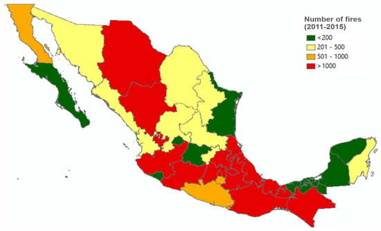
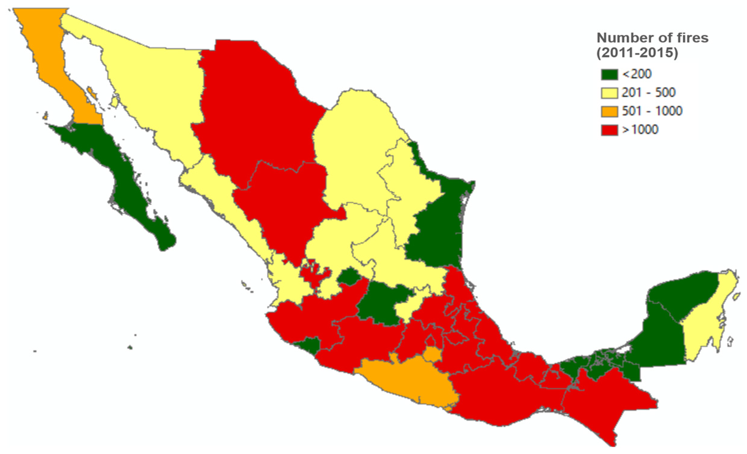
Figure 1.
Number of suppressed fires by state in the study period (2011–2015).
We analyzed fire suppression records from CONAFOR [64] from 2011 to 2015 for every state of Mexico. The database contains the start and end date of each fire, based on fire suppression records, their coordinates, and the corresponding state of Mexico. The total number of fire suppression records in the study period was 38,715. The states with a higher number of fire records included State of Mexico, Chihuahua, Durango, Michoacan, Ciudad de Mexico, Jalisco, Puebla, Chiapas, and Oaxaca, with more than 1000 fire suppression records for the study period (Figure 1). Conversely, the states with the lower number of fire registers were Aguascalientes, Baja California Sur, Colima, Campeche, Guanajuato, Tamaulipas, Tabasco, and Yucatan (Figure 1).
2.2. Fuel Dryness Index
2.2.1. Inputs for the Fuel Dryness Index (FDI) Calculation
The two inputs for FDI calculation, moisture content of dead fuels of 100 h (H100) and 10-day NDVI composites, were supplied by the National Commission for the Knowledge and Use of Biodiversity (CONABIO), as detailed by Cruz-Lopez et al. [74]. H100 composites at 1 km pixel were calculated by CONABIO using the methodology of Cervera-Tavoada [75] to implement the NFDRS of dead fuel moisture content calculation [76] from MODIS temperature and relative humidity and TRMM precipitation [74]. The period of study was 2011–2015, defined by the availability of H100 data from CONABIO at the time of analysis.
The 10-day cloud-free NDVI composite images, with a pixel of 1 km, were calculated from MODIS by CONABIO [74]. The process of gap filling to reconstruct cloud-free NDVI composites was performed by CONABIO using the HANTS (Harmonic Analysis of Time Series) algorithm [77]. HANTS is a widely used algorithm to reconstruct time series for seasonal stationary variables such as NDVI [78]. The algorithm was applied to a time series of 9 years of MODIS NDVI to obtain a fitted time series (using a superposition of periodic functions [77]) to reconstruct the temporal gaps for each pixel.
2.2.2. Fuel Dryness Index (FDI) Calculation
The Fuel Dryness Index (FDI) was calculated using the procedure described by [26] to calibrate the Fire Potential Index (FPI) from Burgan et al. [49] for Mexican ecosystems:
where:
FDI = (1 − LR)·(1 − MR)·100
LR: Live ratio calculated using Equations (2)–(4).
MR: Dead fuels moisture ratio calculated using Equation (5).
FDI is an integrated index that combines both estimates of live fuel moisture (LR) (Equation (1) through (4)) and dead fuel Moisture Ratio (MR) (Equations (1) and (5)), with a spatial resolution of 1 km. It reaches values close to 100 when the pixel reaches its maximum fuel dryness (minimum dead and fuel moisture). Conversely, its lowest values are reached when both live and dead fuels have high moisture [49].
The first component, Live Ratio (LR), was calculated using Equations (2) and (3):
where: RG is Relative Greenness, estimated as:
where: NDVI is the observed 10-day NDVI for each pixel, NDVImin and NDVImax are the minimum and maximum NDVI values for each pixel from the period of study.
LR = RG·LRmax/100
RG = (NDVI − NDVImin)/(NDVImax − NDVImin)·100
LRmax is the maximum Live Ratio value for each pixel, calculated using Equation (4):
where: NDVImax = maximum NDVI for every pixel.
LRmax = 30 + 30·(NDVImax − 125)/(255 − 125)
The values of NDVI were scaled from 0 to 255 to permit data compression, as detailed in [79]. The map of the maximum NDVI observed for each pixel in the study period ranged from 125 to 255 [26]. Following [79], the absolute minimum (125) and maximum (255) values of the maximum NDVI were included in Equation (4).
The value of 30, at the intercept of Equation (4), represents the minimum LRmax value, as established by [79]. Following Equation (4), a maximum LRmax value of 60 is reached for the pixels where the maximum NDVI value reaches its absolute observed value for the study area. Consequently, as proposed for FPI [61,79], areas with a lower maximum NDVI (e.g., desert shrublands) have a lower maximum live ratio (fraction of fuels that is estimated to be alive) and the contrary occurs in areas with higher NDVImax.
Finally, the dead fuel Moisture Ratio (MR) was calculated following Equation (5):
where: H100: observed 100 h dead fuel moisture; Hmax, Hmin: maximum and minimum historical H100 values for each pixel.
MR = (H100 − Hmin)/(Hmax − Hmin)
2.2.3. Accumulated FDI
We tested accumulated FDI (AcFDIi), calculated as the average FDI value for the evaluated i periods of 10, 20, 30, 40, 50, 60, 70, 80, and 90 days, for every Mexico state. Evaluated periods of 10–90 days for the AcFDIi were selected based on the more common range of accumulated periods for fire danger indices considered in the literature (e.g., [17,18]). The index AcFDI was assumed to be zero when the FDI value at the corresponding 10-day period was below a threshold FDI99. For each state, FDI99 thresholds were calculated as the FDI value above which 99% of the fire suppression registers were registered. The average AcFDI was calculated for each state for every period of 10 days in the study period.
2.3. Models for Prediction of Number of Fires for Each State
We evaluated linear and non-linear models to predict the observed number of fires for 10 days for each state from AcFDI and the observed number of fires in the last 10 days. For the non-linear models, we fitted the following expression [26]:
where: NFt: Observed number of fires for each state for each 10-day period t of the study period; AcFDIit: Accumulated Fuel Dryness Index at each 10-day period t of the study period for the evaluated accumulated period i (Section 2.2.3); NFt − 1: Observed number of fires for each state for the previous 10-day period t − 1; a, b, are model coefficients for the role of AcFDI, fitted using non-linear quantile regression at a 95% percentile, and c is a model coefficient to account for the temporal autocorrelation of NF, which was estimated as the calculated correlation coefficient between observed values of NFt and NFt − 1 for each state following [26].
NFt = a·AcFDIit b + c·NFt − 1
For obtaining the a and b model coefficients of AcFDI for each state, we fitted the models from Equation (6) using non-linear quantile regression at a 95% percentile using the R package nlrq [80]. Candidate models were evaluated by means of the coefficient of determination for non-linear regression (R2) (e.g., [81]), defined as the squared correlation coefficient between the measured and estimated values, together with the Root Mean Square Error (RMSE) and model bias.
2.4. Autoregressive Integrated Moving Average (ARIMA) Models to Forecast AcFDI
For the selected AcFDIi index, we evaluated seasonal AutoRegressive (AR) Integrated (I) Moving Average (MA) models (ARIMA) to forecast the AcFDIi for the next 10 days for each state, based on previously observed lags of the same index. Seasonal ARIMAs are frequently used to forecast time series of remotely sensed estimates of fuel moisture such as NDVI (e.g., [82]). They have been previously used to model FPI temporal dynamics by Huesca et al. [53,54].
A generic notation of ARIMA models can be written as:
where: ar = non-seasonal AR lag order, dif = non-seasonal differencing, ma = non-seasonal MA lag order, sar = seasonal AR lag order, sdif = seasonal differencing, sma = seasonal MA lag order, and S = time span of repeating seasonal pattern.
ARIMA (ar, dif, ma) × (sar, sdif, sma)S,
Lag order and components of ARIMA models were identified by an exploratory analysis using auto.arima [53] in R ([83,84]). The most suitable model was selected based on Standard AIC [85], together with the evaluation of model R2, RMSE, and bias. Selected models were fitted using auto.arima in the library forecasting in R ([83,84]). The adequacies of selected models were further evaluated by means of the Ljung–Box Q-statistic [53,86].
For example, if auto.arima selected a (2, 0, 0) × (0, 0, 0)S as the best model, which is an autoregressive model to predict AcFDI from the two previous lags, the corresponding AR model can be written as:
where AR1 and AR2 are the autoregressive AcFDI observed values for lag 1 (i.e., previous 10 days) and lag 2 (previous 11–20 days), respectively, and a0, a1, and a2 are fitted model coefficients using auto.arima ([83,84]).
AcFDI = a0 + a1·AR1 + a2·AR2
3. Results
3.1. FDI99 Thresholds by State
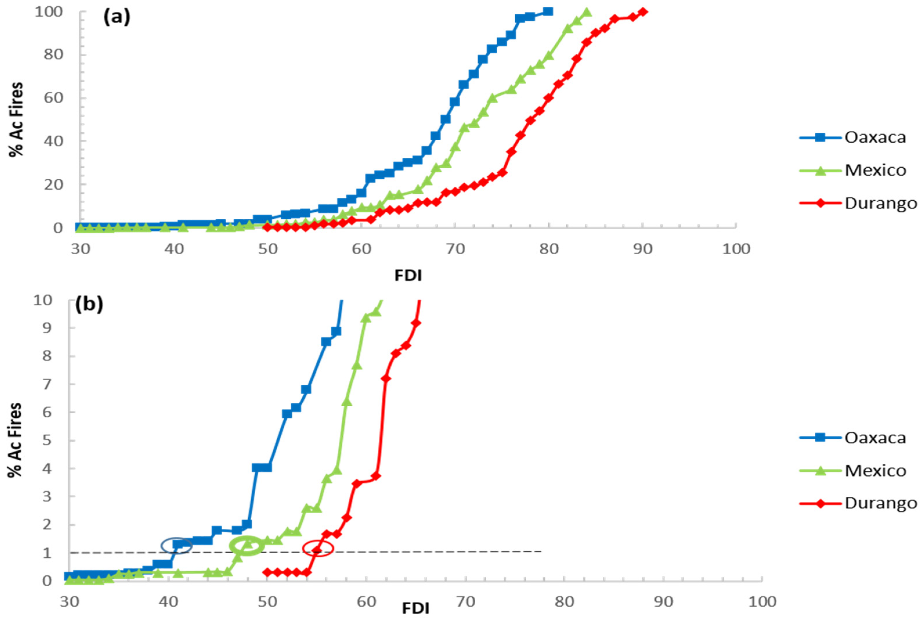
An example of the process of calculation of FDI99 is illustrated in Figure 2. The upper Figure 2a shows the curves of the accumulated percentage of the number of suppressed fires against FDI values. For illustration purposes, we show a selected example for the states of Oaxaca, Durango, and state of Mexico. A detail of the same curves, for the accumulated percentages of fires below 10%, is shown in Figure 2b. FDI99 values, obtained as the nearest FDI integer for the accumulated % fires for the first 1% (i.e., 99% of fires occur above this FDI), are marked in circles for each curve in Figure 2b. FDI99 values of 40, 48, and 55 were obtained for the states of Oaxaca, Mexico, and Durango, respectively (Figure 2b).
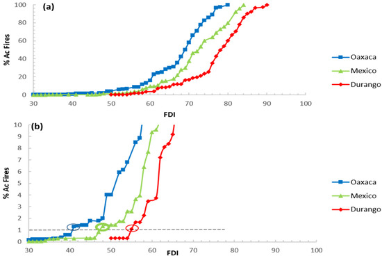
Figure 2.
Accumulated percentage of fires (% Ac Fires) against Fuel Dryness Index (FDI) values for the states of Oaxaca (blue), Durango (red), and State of Mexico (green) (a) and detail of the same curves for the % Ac Fires below 10% (b). FDI99 values (FDI values corresponding to a % Ac Fires of 1) are marked as circles for each curve.
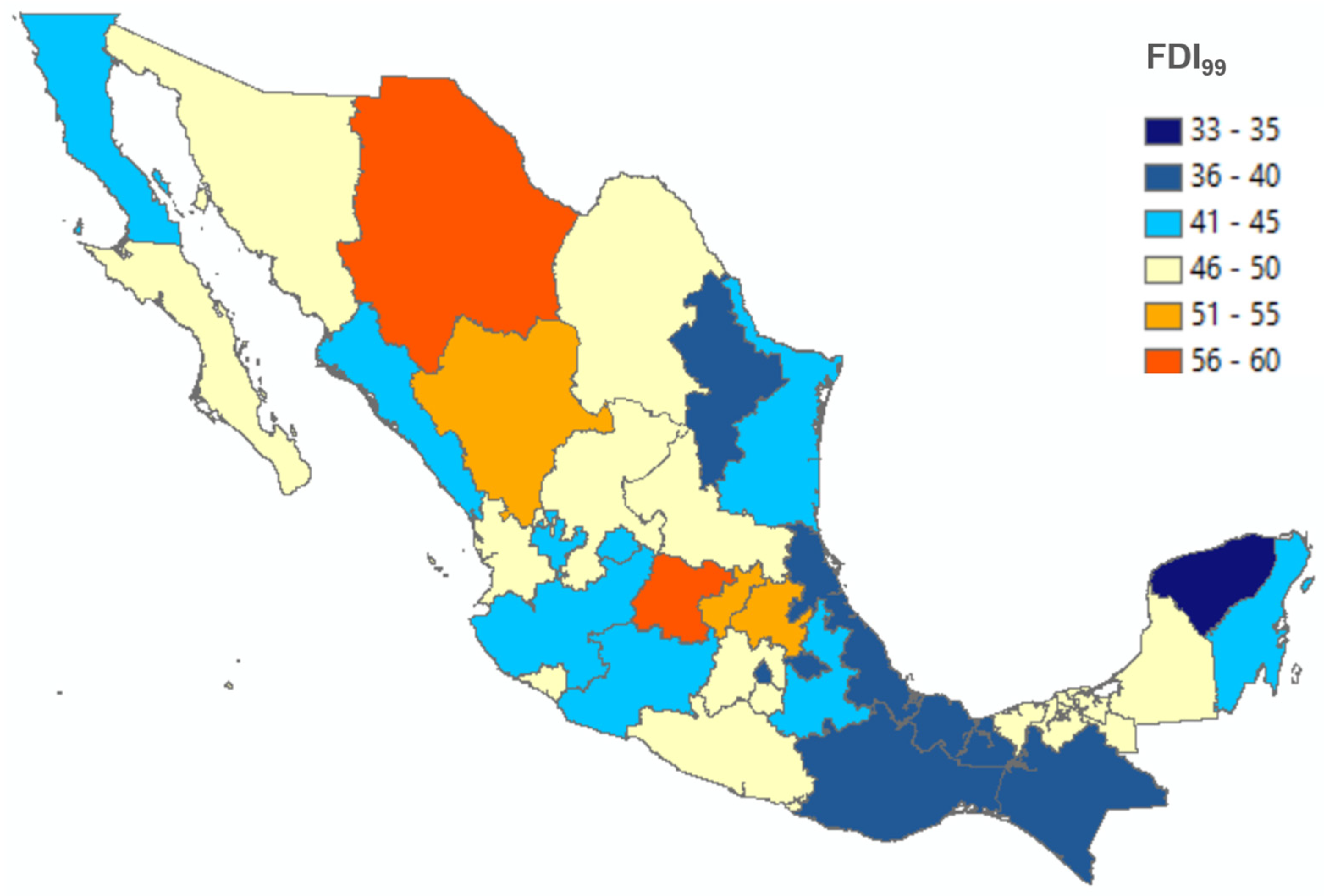
The observed FDI99 values for all the states ranged from 33 to 60 (Figure 3, Table 1). The lowest FDI99 values (<40) were observed in some of the wetter states of the southeast, such as Yucatan, Chiapas, or Oaxaca. On the contrary, higher FDI99 values (>50) were observed for the driest states in the Northern region (e.g., Durango, Chihuahua), or Center (e.g., Hidalgo, Guanajuato, San Luis Potosi).
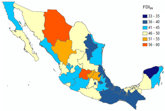
Figure 3.
Map of FDI99 values by state of Mexico.

Table 1.
Coefficient and goodness of fit of models to predict number of fires in 10 days by state.
3.2. Models to Predict Number of Fires by State
Based on a preliminary correlation analysis between the candidate accumulated FDI for the evaluated periods of 10–90 days and the observed number of fires, a period of 50 days was selected for the accumulated Fuel Dryness Index (FDI50) based on an observed higher correlation to predict fire activity for the majority of the analyzed states. The best fits were obtained using non-linear models (Equation (6)). The coefficients and goodness of fit for the models to predict the number of fires from FDI50 using Equation (6) are shown in Table 1. For 19 of the 32 evaluated states, values of R2 higher than 0.4 were observed (Table 1).
In general, the best performance (R2 of up 0.6–0.75) was observed in states with higher fire activity (states with >1000 fires in the study period, Figure 1), such as Chihuahua, Ciudad de Mexico, Jalisco, Michoacan, or the state of Mexico. Conversely, the lowest goodness of fit was observed for states with a low number of fire suppression records (<200 fires in Figure 1), such as Colima, Guanajuato, Tamaulipas, or Yucatan (Table 1). For the two states with very low fire activity, Southern Baja California and Aguascalientes, R2 values lower than 0.1 (models not shown) were obtained. The fitted models from the nearest states (Baja California and Zacatecas, respectively), scaled by the corresponding forest land surface, were applied for those two states. Because of the use of percentile regression, all models showed negative bias values (i.e., the models rarely provide underestimations, as required for risk assessment).
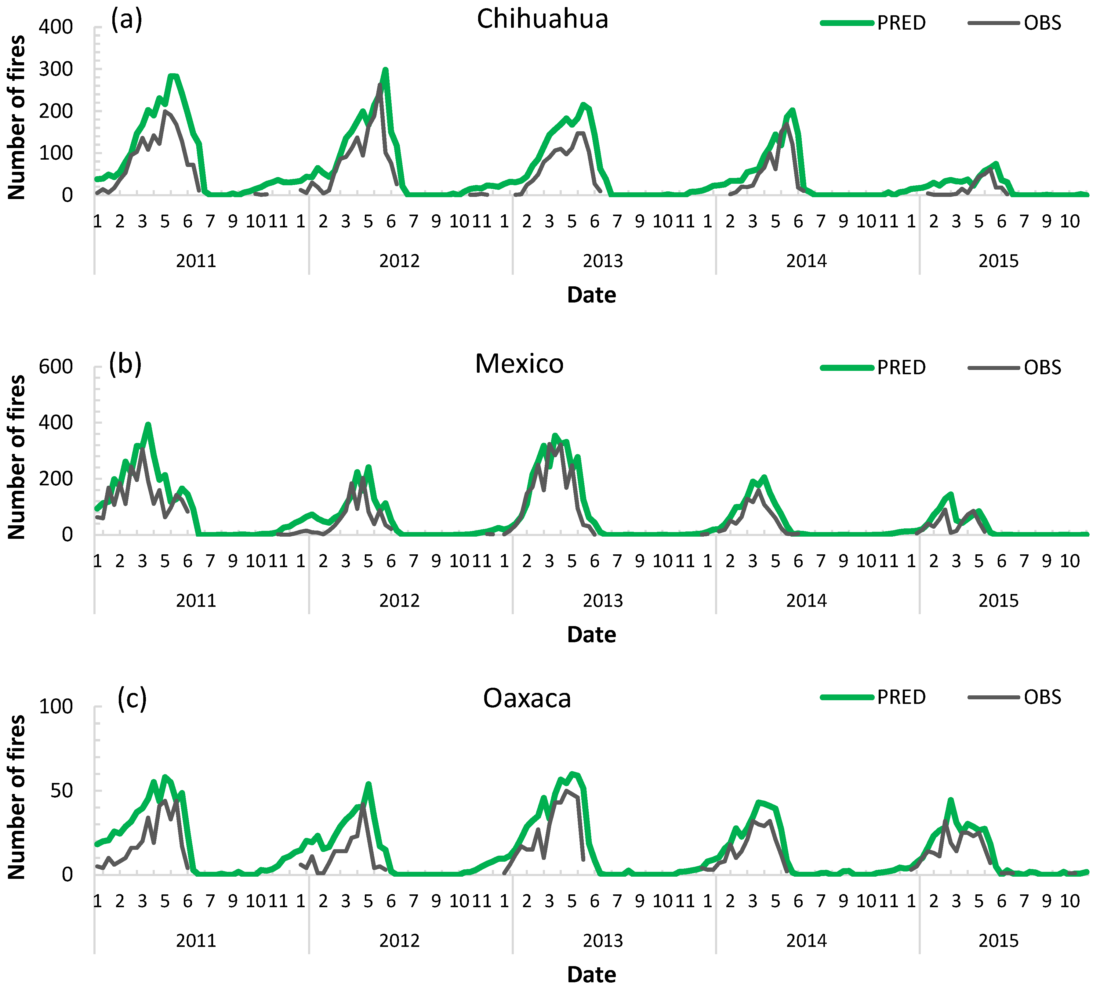
Selected examples of predicted against the observed number of fires in 10 days are shown in Figure 4 for the states of Chihuahua (North region), Mexico (Centre), and Oaxaca (South region). In general, the models provide conservative predictions, with relatively few underestimates, because of the use of percentile regression (to represent “worst case scenarios”), combined with the consideration of autocorrelation, that corrects for unexpected punctual events (i.e., high observed fire activity under relatively wet conditions), that are considered in the prediction for the next 10 days. Additional examples of predicted against observed number of fires are shown in Supplementary Figures S1–S5.
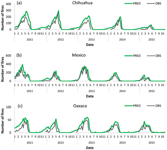
Figure 4.
Selected examples of observed and predicted number of fires in 10 days for the states of Chihuahua (a), State of Mexico (b), and Oaxaca (c). Where PRED: predicted with models from Table 1; OBS: observed.
3.3. Autoregressive Models to Forecast Accumulated Fuel Dryness
Based on the exploratory analysis using autoarima, autoregressive models of order 2, i.e., (2, 0, 0) × (0, 0, 0)S (Equation (8)), were selected. The coefficients for the selected models using Equation (8) to forecast FDI50 are shown in Table 2. R2 ranged from 0.989 to 0.813 and RMSE from 1.70 to 7.54. For 29 out of the 32 evaluated states, R2 values were higher than 0.95 and RMSE values were lower than 2.5. In addition, all the fitted models demonstrated a lack of autocorrelation in the residues based on the Box–Ljung test.
Table 2.
Coefficient and goodness of fit of autoregressive models to forecast accumulated fuel dryness FDI50.
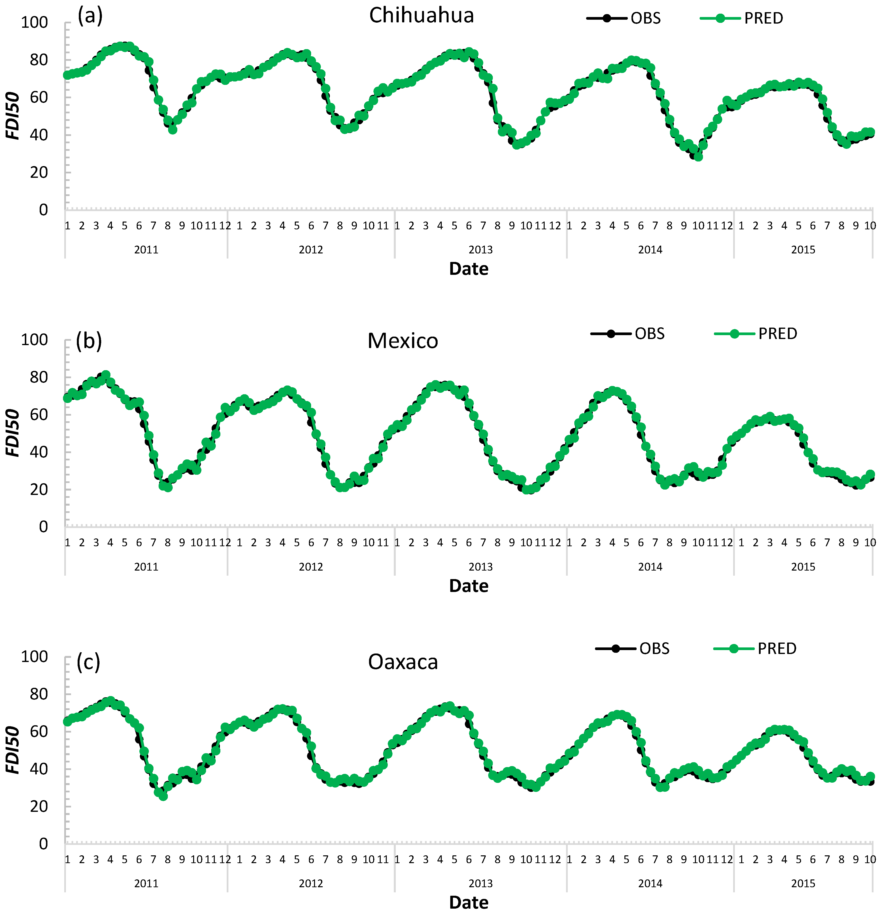
Selected examples of observed against predicted FDI50 values using the fitted autoregressive models are shown in Figure 5, where a close agreement between forecasted and observed fuel dryness can be observed. Plots of observed against predicted FDI50 values for all the evaluated states are shown in Supplementary Figures S6–S10.
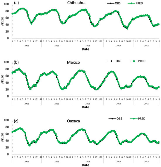
Figure 5.
Selected examples of observed and predicted accumulated fuel dryness FDI50 for the states of Chihuahua (a), State of Mexico (b), and Oaxaca (c).
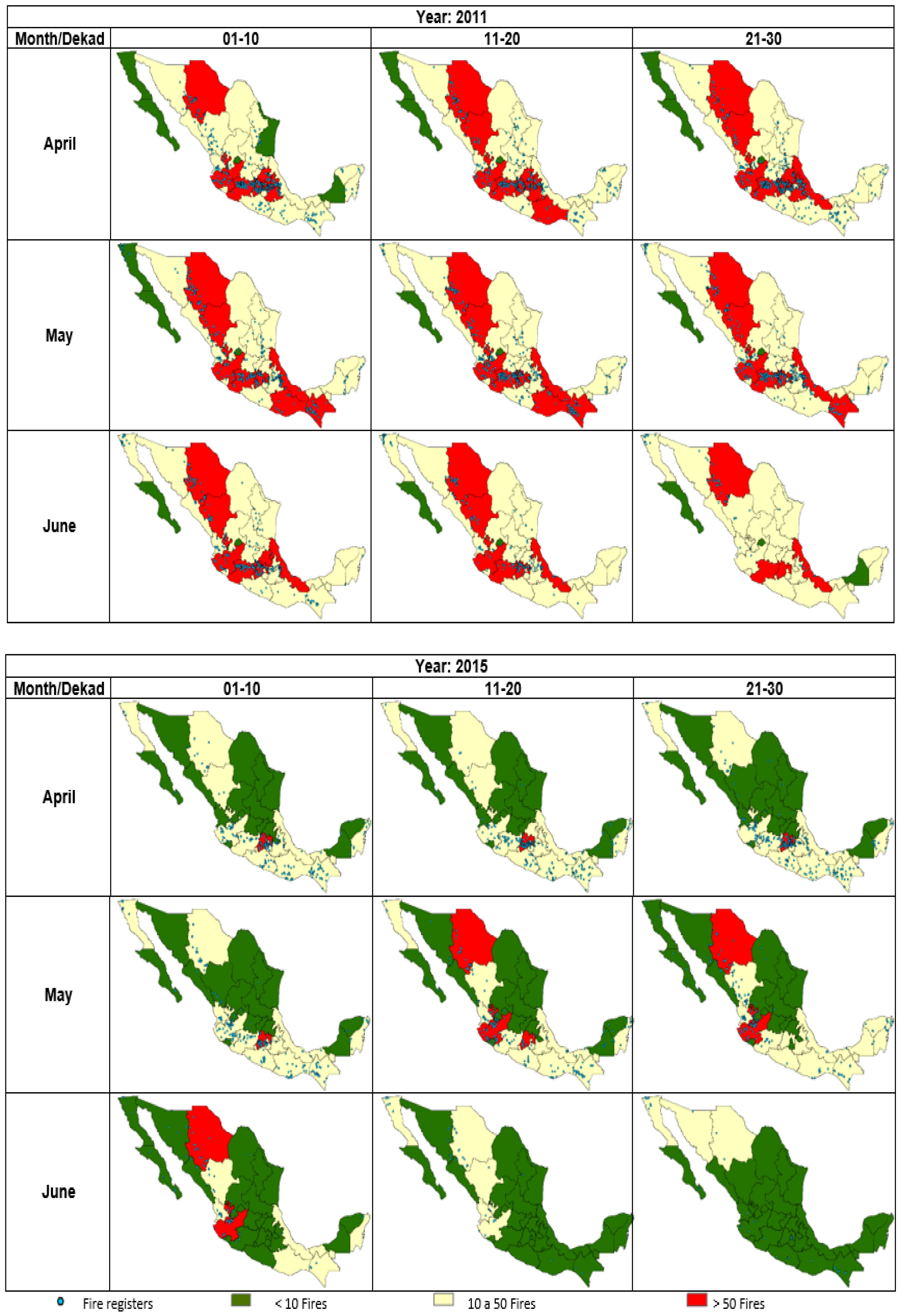
The developed models allow us to map the estimated number of fires by state for every 10-day period, based on the forecasted accumulated fuel dryness FDI50 and on the observed number of fires from the previous 10 days. An example of the forecasted number of fires for two contrasting years (dry year 2011 and wet year 2015) is shown in Figure 6. The forecasted number of fires shows sensitivity to both years and time periods within years of contrasting fuel dryness and previous fire activity, generally matching with observed fire suppression registers (shown as blue dots in Figure 6).

Figure 6.
Predicted number of fires by state for the period April–June of 2011 (three upper rows) and 2015 (three lower rows). Observed fire suppression registers are shown as blue dots in each figure.
4. Discussion
This study demonstrated the potential of the combination of forecasts of remotely sensed fuel moisture, together with autoregressive models that account for human-caused temporal variations in fire activity, to predict fire occurrence at temporal (10 days) and spatial units relevant for fire management planning.
Regarding the analyzed effect of fuel dryness, the observed variations between states in the FDI99 thresholds (Figure 2) in the current study support previous observations that fuel dryness thresholds for fire occurrence can vary between geographical regions (e.g., [87]). Furthermore, the generally lower thresholds for fire occurrence observed in wetter states and, conversely, higher FDI99 found for drier states, support similar previous observations for FPI by [60], who documented the highest FPI thresholds for the drier bioclimatic regions in Southern Europe. This also agrees with previous observations of higher thresholds of live fuel moisture for fire occurrence in drier ecosystems than in wetter, more productive forests (e.g., [40,43,88]).
For several states, the developed models showed some skill in relating the higher observed fire activity (e.g., years 2011–2013 for Chihuahua, Figure 4a) to corresponding higher accumulated fuel dryness in those periods (corresponding years and state in Figure 4a) and, conversely, in explaining the lower fire activity observed in wetter years (e.g., year 2015 for Chihuahua or Mexico, Figure 4a and Figure 5a). This interannual variability in fire activity has been previously documented to be related to annual ENSO indices for Mexico (e.g., [89,90,91]) and other countries (e.g., [92,93,94]), although the country- and region-specific effects of Niño/Niña are still not fully understood for many areas of Mexico (e.g., [95,96,97]). The temporal patterns of observed fire activity (Figure 4 and Supplementary Figures S1–S5) and fuel dryness (Figure 5 and Supplementary Figures S6–S10) point that, for several states in the analysis, particularly in the North of Mexico, higher fire activity is observed for La Niña years, such as 2011, which had been documented to be a record for both number of fires and burned area in Mexico [64].
Our selection of an accumulated fuel dryness index for prediction of fire occurrence seems to agree with studies that have observed higher correlations of fire activity with longer time lag fire weather indices (e.g., [35,98,99]), reinforcing the hypothesis that antecedent water balance and accumulated drought can influence fire activity (e.g., [3,32,33,100]). Interestingly, the selected period of 50 days, out of the candidate 10–90 days evaluated, corresponds directly with the time lag of some frequently used indices that have been found to be related to fire activity, such as Drought Code (DC) (with a time lag of 52 days) ([35,99,101]), 1000 h dead fuel moisture ([17,18]), or 2-month SPI [36]. Furthermore, some of the shorter time lag widely used fire danger indices that have been frequently related to fire activity such as FWI (e.g., [31,37,102]) or ERC (e.g., [4,8]) integrate those longer time lag codes into their weighted calculation (e.g., [2,15]). For example, the 52-day time lag index Drought Code is weighted with 15-day DMC in the FWI calculation through its contribution to the Build-Up Index (BUI) [15]. BUI and DC are commonly used indicators of potential fuel available for surface fuel consumption, allowing fire managers to evaluate the difficulty in finally extinguishing all areas where the fire is smoldering (e.g., [15]). The index ERC is generally calculated for fuel model G (e.g., [2,4,8]), which, owing to a heavy weighting of large dead fuels (100 and 1000 h), is mainly driven by weather conditions during the previous 1.5 months [2].
Beyond a potential influence on coarse dead fuel moisture or on deep soil layers, it is likely that the apparent advantage of the selection of a 50-day period might be related to live fuel moisture dynamics, which are known to influence fire occurrence and spread (e.g., [39,43,103]), although its mathematical contribution to fire modeling remains still as an open research question (e.g., [38,42,43]). In this sense, unlike short-term fire danger indices and dead fuel moisture codes that are driven mainly by short-term weather conditions, live fuel moisture depends not just on recent hydrometeorology [38]. Accumulated vegetation stress is also driven by dynamic and non-linear interactions between weather conditions, soil properties, and plant physiological processes (e.g., [40,42,43]). Plant responses to drought and dry mass changes associated with phenology are particularly critical ([38,42,104]).
This study offers useful information for a hybrid index that, unlike studies that have focused on weather-driven fire danger indices only (e.g., [22,23,37]]) or only on remotely sensed estimates of live fuel moisture (e.g., [39,43,46]), combines both moisture components. This is, to our best knowledge, the first study analyzing several accumulation periods from 10 to 90 days for FPI, one of the few operational fire danger indices integrating both weather-driven dead fuel moisture and remotely sensed live fuel moisture estimates.
Other studies have found the benefit of using time lags beyond 2 months, such as the Monte Alegre formula [105,106], the Telicyn Logarithmic Index [107], and the Nesterov index [108], that use the consecutive number of days without rainfall at longer time periods. Also, the Risco do Fogo index, which considers precipitation over a period of 120 days [109]. However, we did not observe gains using longer accumulation times in our study, with correlations generally decreasing for the 90-day interval period.
In addition, our observed non-linearity in the relationship between accumulated FDI and fire activity from our study supports similar observations for FPI in Europe by [52]. This response has also been observed for other fire weather indices (e.g., [2,102,110]) or for live fuel moisture (e.g., [103]). Consequently, as stated by Koh et al. [111], the common practice of using fire weather indices directly as a proxy for wildfire activity, without a non-linear region-specific calibration to observed fire data, can have limitations in predicting fire occurrence.
This furthermore highlights the need to develop regionally specific calibrated models to convert fire weather indices into estimates of fire activity (e.g., [8,51]). Our high variability in the coefficients to predict fire occurrence might be related to the ample variations in ecosystem types, climate, and human factors between the analyzed states. This corroborates previous observations of variations in such relationships between different regions (e.g., [23,102,112]).
The observed best performance (R2 of >0.6–0.75) in larger states with higher fire activity such as Chihuahua, Ciudad de Mexico, Jalisco, Michoacan, or the State of Mexico, seems to support similar previous observations of stronger relationships at larger areas of study [105]. In general, the range of R2 for the percentile regression models from our study was similar to that found in studies predicting the number of fires in other regions, such as the range of R2 of 0.26–0.46 by [113] or R2 of 0.37–0.60 by [114].
Our observed lower relationship between fuel dryness and fire activity in some of the drier states (e.g., Southern Baja California, Aguascalientes, Sonora, San Luis Potosi, Queretaro, or Guanajuato) agrees with previous studies reporting weaker fuel be related to the observations from previous studies that have similarly documented weaker fuel dryness–fire activity correlations for drier climate regions (e.g., [23,31,37,105]). This might support the hypothesis of varying constraints of fire occurrence (e.g., [115,116]). In addition, weaker weather-fire relationships may arise in regions where fire occurrence is strongly determined by episodic wind-driven fires, such as in Baja California, where Santa Ana winds are known to influence fire activity [117]. Current ongoing research aimed at developing a windy FPI for Mexico, similar to what recently developed for a revised FPI index including wind in the USA [118] or other countries [119] might contribute to improving our capacity to predict fire occurrence in future studies. This could provide information at finer temporal scales than the periods of 10 days evaluated in the current study. In this regard, different time lags of fuel moisture than the ones selected for 10-day fire occurrence here, together with the consideration of wind, might be useful for future analyses aiming at predicting daily fire spread. In addition, future studies could expand the period of study, based on the future availability of FDI data.
Beyond observing the effect of fuel dryness in promoting fire activity, for many of the analyzed states, a large effect of temporal autocorrelation was also documented. For example, in spite of lower observed accumulated fuel dryness in 2015 for the state of Oaxaca (Figure 4c), the relatively large fire observed activity could be generally predicted, even under wetter conditions, because of the consideration of autocorrelation terms. This approach predicts a higher number of fires as a response to observed fire activity from the previous 10 days (Figure 4c). In this sense, many of the states with the largest c coefficient in the predictive equation to account for temporal autocorrelation of previous fire activity (Table 1), such as Oaxaca, Chiapas, Michoacan, Jalisco, or Nayarit, correspond to areas in the center and southeast of Mexico where fires are most likely a result of the spread of frequent agricultural burns (e.g., [120,121]). These observations support the notion that anthropogenic factors can effectively mask or have an influence beyond weather–fire relationships in some regions due to extensive and regular intentional human ignitions where conversion to agricultural lands and greater land fragmentation occurs (e.g., [23,61,62,63]).
Our use of an autoregressive term of 1 lag, allowing us to forecast the number of fires based on the observed number from the previous 10 days, agrees with the observations of [65] who found a temporal correlation of up to 11 days to predict daily arson ignition counts in Florida. Nevertheless, our study, unlike the univariate autoregressive approach of Prestemon et al. [66] or other authors [67,68], or unlike the majority of literature that have used fire danger indices only (e.g., [23,37,102]), included a combination of both fuel dryness and autoregressive terms of previous fire activity, to forecast fire activity of the next 10 days.
In our study, on the one hand, autocorrelation alone explained a relatively large variability of the observed number of fires for the majority of the evaluated states, as noted by a correlation coefficient (c, Table 1) of up to 0.8, being >0.5 for 20 of the analyzed states. On the other hand, adding fuel dryness in addition to autocorrelation improved the correlation for the large majority of the analyzed states (Table 1). For example, in the Campeche state, considering only autocorrelation resulted in an R2 (squared correlation coefficient of 0.40) of 0.16 (Table 1). Conversely, including fuel dryness in addition to autocorrelation increased the R2 for this state to 0.45 (Table 1). Furthermore, using previous fires only, would not allow us to anticipate either (1) the beginning of the fire season (when previous days show few or no fire activity), nor (2) sudden peaks of fire activity when weather conditions aggravate, after previous days of moderate fire activity. This can be observed in the plots of predicted fire activity (Figure 1). For example, for Chihuahua (Figure 4a), at the beginning of the fire season of the year 2012, the previously observed number of fires from the previous month of December 2011 was 0. Using only an extrapolation of the previous fires, one would assume 0 fires for the first 10 days of January, underestimating the observed start of the fire season on this date. Instead, because the model provides a conservative (percentile-fitted) estimate of fire activity based on accumulated fuel dryness, the observed number at the beginning of the fire season is not underestimated (Figure 4a). Also, the sudden increases in fire activity at the end of January 2012 and the start of March 2012 in this state (Figure 4a), which would have otherwise been underestimated based on previously observed fire activity, were successfully anticipated in the predictions because of the consideration of accumulated fuel dryness. This suggests that considering a percentile fit of fire activity against fire weather can provide conservative estimates of fire activity, anticipating sudden peaks of fire occurrence in dry seasons before they have occurred (Figure 4), as desired for a safe fire hazard decision support tool.
Autoregressive terms were also used to forecast the accumulated fuel dryness of the next 10 days. Our approach agrees with the results of Huesca et al. [53] who used autoregressive models of the previous 2 lags to predict FPI in Spain. Although the autoregressive models developed in this study showed good skill (R2 of 0.989 to 0.813) in forecasting the accumulated fuel dryness of the next 10 days, future studies could further explore the use of weather forecasts (e.g., [4,122]). Such approaches could be valuable to predict fire occurrence under potentially changing climate conditions [9,10,11,12], including expanded fire seasons, or changes in the timing of precipitation, that might be better captured with such more detailed weather forecasts.
The current study aimed at forecasting the total number of fires by state. Nevertheless, considering that large fires can represent a large fraction of the fire suppression budget (e.g., [5,123,124,125]), future studies could aim at predicting a number of large fires (e.g., [8]). Furthermore, beyond developing temporal forecasts of large fire activity based on the average (or percentile) fuel dryness value by state, more detailed spatio-temporal approaches to predict fire occurrence, such as those demonstrated by Preisler et al. [8,19]), should be explored in future studies. Such approaches could allow both mapping fire or large fire occurrence probability and simultaneously estimating the number of fires or the number of large fires for a particular region and period of time by summing the estimated probability values of individual voxels (e.g., [51]). This would further contribute to support decision-making not only between but also within states, potentially improving fire suppression and fire management planning.
5. Conclusions
The main conclusions of the study can be summarized as:
- (1)
- This study evaluated for the first time the effect of different accumulation time periods on the capability of a modified version of the FPI fire danger index to forecast the number of fires.
- (2)
- Our results suggest that a period of 50 days, provided the best results to forecast fire activity in a variety of geographical areas with different ecosystems and climates in Mexico. These results indicate a potential effect of the selected time period in capturing live fuel moisture dynamics effects in fire occurrence for the study area analyzed, that could be tested for accumulated FPI in other research areas using the methodology presented here.
- (3)
- In addition, the use of autoregressive terms, in combination with the accumulated fuel dryness, reveals its usefulness for predicting fire activity for several states. This approach could be tested elsewhere based on FPI or other fire indices to forecast fire activity.
- (4)
- Finally, autoregressive models showed good performance in forecasting Accumulated Fuel Dryness (AcFDI) based on previously observed AcFDI values, allowing the development of forecasts of the expected number of fires by state for the next 10 days.
- (5)
- Future studies might enhance the potential of these initial models by exploring weather forecasts of both predicted fuel dryness and wind. Furthermore, spatio-temporal approaches should be also tested to further support fire management planning at different time and spatial scales.
Supplementary Materials
The following supporting information can be downloaded at: https://www.mdpi.com/article/10.3390/f15010042/s1, Figures S1–S5: Observed and predicted number of fires per dekad for the states of Chiapas, Ciudad de Mexico, Durango and Guerrero (S1), Hidalgo, Jalisco, Michoacan and Morelos (S2), Puebla, Nayarit, Queretaro and San Luis Potosi (S3), Sinaloa, Sonora, Tlaxcala, and Veracruz (S4) and Zacatecas, Coahuila, Campeche and Yucatan (S5). Figures S6–S10: Observed and predicted accumulated fuel dryness FDI50 for the states of Chiapas, Ciudad de Mexico, Durango and Guerrero (S6), Hidalgo, Jalisco, Michoacan and Morelos (S7), Puebla, Nayarit, Queretaro and San Luis Potosi (S8), Sinaloa, Sonora, Tlaxcala, and Veracruz (S9) and Zacatecas, Coahuila, Campeche and Yucatan (S10).
Author Contributions
D.J.V.-N., P.-M.L.-S. and J.B.-R. performed the statistical analysis; J.B.-R. programmed the code for the daily Fuel Dryness Index automated calculation and for the extraction of FDI values to the daily fire hotspots; R.E.B. provided the Fire Potential Index algorithm, upon which much of this research is based; M.I.C.-L., M.C. and R.R. calculated daily H100 and 10-day NDVI composites from satellite information from CONABIO; D.J.V.-N., writing—original draft preparation; J.J.C.-R., M.P.-G. and E.A.-C., writing—review and editing. All authors have read and agreed to the published version of the manuscript.
Funding
Funding for this study was provided by CONAFOR/CONACYT Project “CO-2018-2-A3-S-131553, Reforzamiento al Sistema Nacional de Predicción de Peligro de Incendios Forestales de México para el pronóstico de conglomerados y área quemada (2019–2022)”, for the enhancement of the Forest Fire Danger Prediction System of Mexico to map and forecast active fire perimeters and burned area, and by the project CONAFOR/CONACYT Project C0-3-2014 “Development of a Forest Fire Danger Prediction System for Mexico (2015–2017)” for the development of a Forest Fire Danger Prediction System for Mexico, funded by the Sectorial Fund for forest research, development and technological innovation “Fondo Sectorial para la investigación, el desarrollo y la innovación tecnológica forestal”.
Data Availability Statement
Fire suppression registers from CONAFOR can be downloaded from the section “Incendios” of the Forest Fire Danger Forecast System of Mexico, “Sistema de Predicción de Peligro de Incendios Forestales de México” (SPPIF): http://forestales.ujed.mx/incendios2/Fuel (accessed on 20 December 2023) dryness indexes can be visualized in SPPIF and are available upon request to the authors.
Acknowledgments
We want to thank CONAFOR personnel for providing the fire suppression registers analyzed in the study. We also want to thank CONABIO’s personnel for providing us access to the satellite daily data of fire hotspots, 10-day NDVI composites, and daily dead fuel moisture images for Mexico for the period of study.
Conflicts of Interest
The authors declare no conflicts of interest. The founding sponsors had no role in the design of the study; in the collection, analyses, or interpretation of data; in the writing of the manuscript, and in the decision to publish the results.
References
- Littell, J.S.; McKenzie, D.; Peterson, D.L.; Westerling, A.L. Climate and Wildfire Area Burned in Western U.S. Ecoprovinces, 1916–2003. Ecol. Appl. 2009, 19, 1003–1021. [Google Scholar] [CrossRef]
- Riley, K.L.; Abatzoglou, J.T.; Grenfell, I.C.; Klene, A.E.; Heinsch, F.A. The Relationship of Large Fire Occurrence with Drought and Fire Danger Indices in the Western USA, 1984–2008, the Role of Temporal Scale. Int. J. Wildland Fire 2013, 22, 894–909. [Google Scholar] [CrossRef]
- Abatzoglou, J.T.; Kolden, C.A. Relationships between Climate and Macroscale Area Burned in the Western United States. Int. J. Wildland Fire 2013, 22, 1003. [Google Scholar] [CrossRef]
- Jolly, W.M.; Freeborn, P.H.; Page, W.G.; Butler, B.W. Severe fire danger index: A forecastable metric to inform firefighter and community wildfire risk Management. Fire 2019, 2, 47. [Google Scholar] [CrossRef]
- Preisler, H.K.; Westerling, A.L.; Gebert, K.M.; Munoz-Arriola, F.; Holmes, T.P. Spatially Explicit Forecasts of Large Wildland Fire Probability and Suppression Costs for California. Int. J. Wildland Fire 2011, 20, 508–517. [Google Scholar] [CrossRef]
- Rodríguez y Silva, F.; Molina Martínez, J.R.; González-Cabán, A. A Methodology for Determining Operational Priorities for Prevention and Suppression of Wildland Fires. Int. J. Wildland Fire 2014, 243, 544–554. [Google Scholar] [CrossRef]
- Jolly, W.M.; Freeborn, P.H. Towards Improving Wildland Firefighter Situational Awareness through Daily Fire Behaviour Risk Assessments in the US Northern Rockies and Northern Great Basin. Int. J. Wildland Fire 2017, 26, 574–586. [Google Scholar] [CrossRef]
- Preisler, H.K.; Riley, K.L.; Stonesifer, C.S.; Calkin, D.E.; Jolly, W.M. Near-Term Probabilistic Forecast of Significant Wildfire Events for the Western United States. Int. J. Wildland Fire 2016, 25, 1169–1180. [Google Scholar] [CrossRef]
- Dupuy, J.; Fargeon, H.; Martin-StPaul, N.; Pimont, F.; Ruffault, J.; Guijarro, M.; Hernando, C.; Madrigal, J.; Fernandes, P. Climate Change Impact on Future Wildfire Danger and Activity in Southern Europe: A Review. Ann. For. Sci. 2020, 77, 35. [Google Scholar] [CrossRef]
- Coop, J.D.; Parks, S.A.; Stevens-Rumann, C.S.; Ritter, S.M.; Hofman, C.M. Extreme Fire Spread Events and Area Burned under Recent and Future Climate in the Western USA. Glob. Ecol. Biogeogr. 2022, 31, 1949–1959. [Google Scholar] [CrossRef]
- Jolly, W.; Cochrane, M.; Freeborn, P.; Holden, Z.A.; Brown, T.J.; Williamson, G.J.; Bowman, D.M. Climate-Induced Variations in Global Wildfire Danger from 1979 to 2013. Nat. Commun. 2015, 6, 7537. [Google Scholar] [CrossRef]
- Jain, P.; Wang, X.; Flannigan, M.D. Trend analysis of fire season length and extreme fire weather in North America between 1979 and 2015. Int. J. Wildland Fire 2017, 26, 1009. [Google Scholar] [CrossRef]
- Collins, B.M.; Omi, P.N.; Chapman, P.L. Regional Relationships between Climate and Wildfire-Burned Area in the Interior West, USA. Can. J. For. Res. 2006, 36, 699–709. [Google Scholar] [CrossRef]
- Woolford, D.G.; Dean, C.B.; Martell, D.L.; Cao, J.; Wotton, B.M. Lightning-Caused Forest Fire Risk in Northwestern Ontario, Canada Is Increasing and Associated with Anomalies in Fire-Weather. Environmetrics 2014, 25, 406–416. [Google Scholar] [CrossRef]
- Wotton, B.M. Interpreting and Using Outputs from the Canadian Forest Fire Danger Rating System in Research Applications. Environ. Ecol. Stat. 2009, 16, 107–131. [Google Scholar] [CrossRef]
- Johnston, L.M.; Wang, X.; Erni, S.; Taylor, S.W.; McFayden, C.B.; Oliver, J.A.; Stockdale, C.; Christianson, A.; Boulanger, Y.; Gauthier, S.; et al. Wildland fire risk research in Canada. Environ. Rev. 2020, 28, 164–186. [Google Scholar] [CrossRef]
- Zacharakis, I.; Tsihrintzis, V.A. Environmental Forest Fire Danger Rating Systems and Indices around the Globe: A Review. Land 2023, 12, 194. [Google Scholar] [CrossRef]
- Zacharakis, I.; Tsihrintzis, V.A. Integrated Wildfire Danger Models and Factors: A Review. Sci. Total Environ. 2023, 899, 165704. [Google Scholar] [CrossRef]
- Preisler, H.K.; Westerling, A.L. Statistical Model for Forecasting Monthly Large Wildfire Events in Western United States. J. Appl. Meteorol. Clim. 2007, 46, 1020–1030. [Google Scholar] [CrossRef]
- Andrews, P.L.; Loftsgaarden, D.O.; Bradshaw, L.S. Evaluation of Fire Danger Rating Indexes Using Logistic Regression and Percentile Analysis. Int. J. Wildland Fire 2003, 12, 213–226. [Google Scholar] [CrossRef]
- Littell, J.S.; Peterson, D.L.; Riley, K.L.; Liu, Y.; Luce, C.H. A Review of the Relationships Between Drought and Forest Fire in the United States. Glob. Chang. Biol. 2016, 22, 2352–2369. [Google Scholar] [CrossRef]
- Urbieta, I.R.; Zavala, G.; Bedia, J.; Gutiérrez, J.M.; San Miguel-Ayanz, J.; Camia, A.; Keeley, J.E.; Moreno, J.M. Fire Activity as a Function of Fire-Weather Seasonal Severity and Antecedent Climate across Spatial Scales across spatial scales in southern Europe and Pacific western USA. Environ. Res. Lett. 2015, 10, 114013. [Google Scholar] [CrossRef]
- Abatzoglou, J.T.; Williams, A.P.; Boschetti, L.; Zubkova, M.; Kolden, C.A. Global Patterns of Interannual Climate–Fire Relationships. Glob. Chang. Biol. 2018, 24, 5164–5175. [Google Scholar] [CrossRef]
- Cadena Zamudio, D.A.; Guerra, B.R.; Arispe Vázquez, J.L.A.; Flores Garnica, J.G.; Avilés, L.C.; Aguilar, R.T.; Cantú, N.; Bautista, A.A.; Mayo Hernandez, J.; Castillo Quiroz, D.; et al. Trends in Global and Mexico Research in Wildfires: A Bibliometric Perspective. Open J. For. 2023, 13, 182–199. [Google Scholar]
- Manzo-Delgado, L.; Sánchez-Colón, S.; Álvarez, R. Assessment of seasonal forest fire risk using NOAA-AVHRR: A case study in central Mexico. Int. J. Remote Sens. 2009, 30, 4991–5013. [Google Scholar] [CrossRef]
- Vega-Nieva, D.J.; Briseño-Reyes, J.; Nava-Miranda, M.G.; Calleros-Flores, E.; López-Serrano, P.M.; Corral-Rivas, J.J.; Montiel-Antuna, E.; Cruz-López, M.I.; Cuahutle, M.; Ressl, R.; et al. Developing Models to Predict the Number of Fire Hotspots from an Accumulated Fuel Dryness Index by Vegetation Type and Region in Mexico. Forests 2018, 9, 190. [Google Scholar] [CrossRef]
- White, L.A.S.; White, B.L.A.; Ribeiro, G.T. Evaluation of Forest Fire Danger Indexes for Eucalypt Plantations in Bahia, Brazil. Int. J. For. Res. 2015, 2015, 613736. [Google Scholar] [CrossRef]
- Anderson, L.O.; Burton, C.; dos Reis, J.B.; Pessôa, A.C.M.; Bett, P.; Carvalho, N.S.; Junior, C.H.S.; Williams, K.; Selaya, G.; Armenteras, D.; et al. An Alert System for Seasonal Fire Probability Forecast for South American Protected Areas. Clim. Resil. Sustain. 2022, 1, e19. [Google Scholar] [CrossRef]
- Flannigan, M.D.; Logan, K.A.; Amiro, B.D.; Skinner, W.R.; Stocks, B.J. Future Area Burned in Canada. Clim. Chang. 2005, 72, 1–16. [Google Scholar] [CrossRef]
- Magnussen, S.; Taylor, S.W. Prediction of Daily Lightning- and Human-Caused Fires in British Columbia. Int. J. Wildland Fire 2012, 21, 342. [Google Scholar] [CrossRef]
- Jones, M.W.; Abatzoglou, J.T.; Veraverbeke, S.; Andela, N.; Lasslop, G.; Forkel, M.; Smith, A.J.; Burton, C.; Betts, R.A.; van der Werf, G.R.; et al. Global and Regional Trends and Drivers of Fire under Climate Change. Rev. Geophys. 2022, 60, e2020RG000726. [Google Scholar] [CrossRef]
- Keeley, J.E. Impact of Antecedent Climate on Fire Regimes in Coastal California. Int. J. Wildland Fire 2004, 13, 173–182. [Google Scholar] [CrossRef]
- Gedalof, Z.; Peterson, D.L.; Mantua, N.J. Atmospheric, Climatic, and Ecological Controls on Extreme Wildfire Years in the Northwestern United States. Ecol. Appl. 2005, 15, 154–174. [Google Scholar] [CrossRef]
- Girardin, M.P.; Wotton, B.M. Summer moisture and wildfire risks across Canada. J. Appl. Met. Clim. 2009, 48, 517–533. [Google Scholar] [CrossRef]
- Rodrigues, M.; Trigo, R.M.; Vega-García, C.; Cardil, A. Identifying Large Fire Weather Typologies in the Iberian Peninsula. Agric. For. Meteorol. 2020, 280, 107789. [Google Scholar] [CrossRef]
- Gudmundsson, L.; Rego, F.C.; Rocha, M.; Seneviratne, S.I. Predicting above-normal wildfire activity in southern Europe as a function of meteorological drought. Environ. Res. Lett. 2014, 9, 084008. [Google Scholar] [CrossRef]
- Turco, M.; von Hardenberg, J.; AghaKouchak, A.; Llasat, M.C.; Provenzale, A.; Trigo, R.M. On the Key Role of Droughts in the Dynamics of Summer Fires in Mediterranean Europe. Sci. Rep. 2017, 7, 81. [Google Scholar] [CrossRef]
- Ruffault, J.; Martin-StPaul, N.; Pimont, F.; Dupuy, J.-L. How Well Do Meteorological Drought Indices Predict Live Fuel Moisture Content (LFMC)? An Assessment for Wildfire Research and Operations in Mediterranean Ecosystems. Agric. For. Meteorol. 2018, 262, 391–401. [Google Scholar] [CrossRef]
- Maffei, C.; Menenti, M. Predicting Forest Fires Burned Area and Rate of Spread from Pre-Fire Multispectral Satellite Measurements. ISPRS J. Photogramm. Remote Sens. 2019, 158, 263–278. [Google Scholar] [CrossRef]
- Nolan, R.H.; Foster, B.; Griebel, A.; Choat, B.; Medlyn, B.E.; Yebra, M.; Younes, N.; Boer, M.M. Drought-Related Leaf Functional Traits Control Spatial and Temporal Dynamics of Live Fuel Moisture Content. Agric. For. Meteorol. 2022, 319, 108941. [Google Scholar] [CrossRef]
- Rossa, C.G.; Fernandes, P.M. On the Effect of Live Fuel Moisture Content on Firespread Rate. For. Syst. 2017, 26, eSC08. [Google Scholar] [CrossRef]
- Jolly, W.M.; Johnson, D.M. Pyro-ecophysiology: Shifting the Paradigm of Live Wildland Fuel Research. Fire 2018, 1, 8. [Google Scholar] [CrossRef]
- Rao, K.; Williams, A.P.; Diffenbaugh, N.S.; Yebra, M.; Bryant, C.; Konings, A.G. Dry Live Fuels Increase the Likelihood of Lightning-Caused Fires. Geophys. Res. Lett. 2023, 50, e2022GL100975. [Google Scholar] [CrossRef]
- Yebra, D.P.; Chuvieco, E.; Riaño, D.; Zylstra, P.; Hunt, R.; Danson, F.M.; Qi, Y.; Jurdao, S. A Global Review of Remote Sensing of Live Fuel Moisture Content for Fire Danger Assessment, Moving towards Operational Products. Remote Sens. Environ. 2013, 136, 455–468. [Google Scholar] [CrossRef]
- Marino, E.; Yebra, M.; Guillén-Climent, M.; Algeet, N.; Tomé, J.L.; Madrigal, J.; Guijarro, M.; Hernando, C. Investigating Live Fuel Moisture Content Estimation in Fire-Prone Shrubland from Remote Sensing Using Empirical Modelling and RTM Simulations. Remote Sens. 2020, 12, 2251. [Google Scholar] [CrossRef]
- Jurdao, S.; Chuvieco, E.; Arevalillo, J.M. Modelling Fire Ignition Probability from Satellite Estimates of Live Fuel Moisture Content. Fire Ecol. 2012, 8, 77–97. [Google Scholar] [CrossRef]
- Manzo-Delgado, L.; Aguirre-Gómez, R.; Álvarez, R. Multitemporal analysis of land surface temperature using NOAA-AVHRR: Preliminary relationships between climatic anomalies and forest fires. Int. J. Remote Sens. 2004, 25, 4417–4424. [Google Scholar] [CrossRef]
- Abdollahi, M.; Islam, T.; Gupta, A.; Hassan, Q. An Advanced Forest Fire Danger Forecasting System: Integration of Remote Sensing and Historical Sources of Ignition Data. Remote Sens. 2018, 10, 923. [Google Scholar] [CrossRef]
- Burgan, R.E.; Klaver, R.W.; Klaver, J.M. Fuel Models and Fire Potential from Satellite and Surface Observations. Int. J. Wildland Fire 1998, 83, 159–170. [Google Scholar] [CrossRef]
- Schneider, P.; Roberts, D.A.; Kyriakidis, P.C. A VARI-Based Relative Greenness from MODIS Data for Computing the Fire Potential Index. Remote Sens. Environ. 2008, 112, 1151–1167. [Google Scholar] [CrossRef]
- Preisler, H.K.; Burgan, R.E.; Eidenshink, J.C.; Klaver, J.M.; Klaver, R.W. Forecasting Distributions of Large Federal-Lands Fires Utilizing Satellite and Gridded Weather Information. Int. J. Wildland Fire 2009, 18, 508–516. [Google Scholar] [CrossRef]
- Sebastián López, A.; Burgan, R.E.; Calle, A.; Palacios-Orueta, A. Calibration of the Fire Potential Index in Different Seasons and Bioclimatic Regions of Southern Europe. In Proceedings of the 4th Wildland Fire International Conference, Sevilla, Spain, 14–17 May 2007. [Google Scholar]
- Huesca, M.; Litago, J.; Palacios-Orueta, A.; Montes, F.; Sebastián-López, A.; Escribano, P. Assessment of forest fire seasonality using MODIS fire potential: A timeseries approach. Agric. Forest Meteorol. 2009, 149, 1946–1955. [Google Scholar] [CrossRef]
- Huesca, M.; Litago, J.; Merino-de-Miguel, S.; Cicuendez-López-Ocaña, V.; Palacios-Orueta, A. Modeling and forecasting MODIS-based Fire Potential Index on a pixel basis using time series models. Int. J. Appl. Earth Obs. Geoinf. 2014, 26, 363–376. [Google Scholar] [CrossRef]
- Podur, J.; Martell, D.L.; Csillag, F. Spatial patterns of lightning-caused forest fires in Ontario, 1976–1998. Ecol. Model. 2003, 164, 1–20. [Google Scholar] [CrossRef]
- Narayanaraj, G.; Wimberly, M.C. Influence of forest roads on the spatial patterns of human- and lightning- caused wildfire ignition. Appl. Geogr. 2012, 32, 878–888. [Google Scholar] [CrossRef]
- Costafreda-Aumedes, S.; Comas, C.; Vega-García, C. Human-caused fire occurrence odelling in perspective: A review. Int. J. Wildland Fire 2017, 26, 983–998. [Google Scholar] [CrossRef]
- Syphard, A.D.; Brennan, T.J.; Keeley, J.E. Chaparral landscape conversion in southern California. In Valuing Chaparral; Underwood, E.C., Safford, H.D., Molinari, N.A., Keeley, J.E., Eds.; Springer International Publishing: Basel, Switzerland, 2018; pp. 311–334. [Google Scholar]
- Parisien, M.A.; Miller, C.; Parks, S.A.; DeLancey, E.R.; Robinne, F.-N.; Flannigan, M.D. The spatially varying influence of human on fire probability in North America. Environ. Res. Lett. 2016, 11, 075005. [Google Scholar] [CrossRef]
- Tariq, A.; Shu, H.; Siddiqui, S.; Munir, I.; Sharifi, A.; Li, Q.; Lu, L. Spatio-temporal analysis of forest fire events in the Margalla Hills, Islamabad, Pakistan using socio-economic and environmental variable data with machine learning methods. J. For. Res. 2021, 13, 12. [Google Scholar] [CrossRef]
- Andela, N.; Morton, D.C.; Giglio, L.; Chen, Y.; van der Werf, G.R.; Kasibhatla, P.S.; DeFries, R.S.; Collatz, G.J.; Hantson, S.; Kloster, S.; et al. A Human-Driven Decline in Global Burned Area. Science 2017, 356, 1356–1362. [Google Scholar] [CrossRef]
- Syphard, A.D.; Keeley, J.E.; Pfaff, A.H.; Ferschweiler, K. Human Presence Diminishes the Importance of Climate in Driving Fire Activity across the United States. Proc. Natl. Acad. Sci. USA 2017, 114, 13750–13755. [Google Scholar] [CrossRef]
- Pausas, J.G.; Keeley, J.E. Abrupt Climate-Independent Fire Regime Changes. Ecosystems 2014, 17, 1109–1120. [Google Scholar] [CrossRef]
- CONAFOR (Comisión Nacional Forestal). Sistema Nacional de Información Forestal. Available online: https://snif.cnf.gob.mx/incendios/ (accessed on 12 December 2023).
- Prestemon, J.P.; Butry, D.T. Time to Burn: Modeling Wildland Arson as an Autoregressive Crime Function. Am. J. Agric. Econ. 2005, 87, 756–770. [Google Scholar] [CrossRef]
- Prestemon, J.F.; Chas-Amil, M.L.; Touza, J.M.; Goodrick, S.L. Forecasting Intentional Wildfires Using Temporal and Spatiotemporal Autocorrelations. Int. J. Wildland Fire 2012, 21, 743–754. [Google Scholar] [CrossRef]
- Slavia, A.P.; Sutoyo, E.; Witarsyah, D. Hotspots Forecasting Using Autoregressive Integrated Moving Average (ARIMA) for Detecting Forest Fires. In Proceedings of the IEEE International Conference on Internet of Things and Intelligence System (IoTaIS), Bali, Indonesia, 5–7 November 2019. [Google Scholar] [CrossRef]
- Kadir, E.A.; Dayana, N.E.; Rosa, S.L.; Othman, M.; Saian, R. Prediction of Hotspots in Riau Province, Indonesia Using the Autoregressive Integrated Moving Average (ARIMA) Model. SAR J. 2020, 3, 101–110. [Google Scholar] [CrossRef]
- Shabbir, A.H.; Zhang, J.; Liu, X.; Lutz, J.A.; Valencia, C.; Johnston, J.D. Determining the Sensitivity of Grassland Area Burned to Climate Variation in Xilingol, China, with an Autoregressive Distributed Lag Approach. Int. J. Wildland Fire 2019, 28, 628–639. [Google Scholar] [CrossRef]
- Shabbir, A.H.; Zhang, J.; Johnston, J.D.; Sarkodie, S.A.; Lutz, J.A.; Liu, X. Predicting the Influence of Climate on Grassland Area Burned in Xilingol, China with Dynamic Simulations of Autoregressive Distributed Lag Models. PLoS ONE 2020, 15, e0229894. [Google Scholar] [CrossRef]
- Kale, M.P.; Mishra, A.; Pardeshi, S.; Ghosh, S.; Pai, D.S.; Roy, P.S. Forecasting Wildfires in Major Forest Types of India. Front. For. Glob. Chang. 2022, 5, 882685. [Google Scholar] [CrossRef]
- INEGI (Instituto Nacional de Estadística y Geografía-México). Guía Para la Interpretación de Cartografía: Uso del Suelo y Vegetación. Escala 1,250,000; Serie VI; Instituto Nacional de Estadística y Geografía: Ciudad de México, Mexico, 2014. [Google Scholar]
- Aguilar-Barajas, I.; Sisto, N.P.; Magaña-Rueda, V.; Ramírez, A.I.; Mahlknecht, J. Drought policy in Mexico: A long, slow march toward an integrated and preventive management model. Water Policy 2016, 18, 107–121. [Google Scholar] [CrossRef]
- Cruz-Lopez, M.I. The National System for Satellite based real-time wildfire monitoring. In Latin America Geospatial Forum; INEGI: México City, Mexico, 2014. [Google Scholar]
- Cervera-Taboada, A. Implementación de un modelo para estimar la humedad en el combustible muerto, basado en datos de sensores remotos. In Reporte de Investigación Grado de Licenciatura; UNAM: México City, Mexico, 2009. [Google Scholar]
- Fosberg, M.A. Moisture Content Calculations for the 100-Hour Timelag Fuel in Fire Danger Rating; Research Note RM-199; USDA Forest Service, Rocky Mountain Forest and Range Experimental Station: Fort Collins, CO, USA, 1971. [Google Scholar]
- Zhou, J.; Jia, L.; Menenti, M. Reconstruction of global MODIS NDVI time series: Performance of Harmonic ANalysis of Time Series (HANTS). Rem. Sens. Environ. 2015, 163, 217–228. [Google Scholar] [CrossRef]
- Roerink, G.J.; Menenti, M.; Verhoef, W. Reconstructing cloudfree NDVI composites using Fourier analysis of time series. Int. J. Rem. Sens. 2000, 21, 1911–1917. [Google Scholar] [CrossRef]
- Sudiana, D.; Kuze, H.; Takeuchi, N.; Burgan, R.E. Assessing forest fire potential in Kalimantan Island, Indonesia, using satellite and surface weather data. Int. J. Wildland Fire 2003, 12, 175–184. [Google Scholar] [CrossRef]
- Koenker, R.; Park, B.J. An Interior Point Algorithm for Nonlinear Quantile Regression. J. Econom. 1994, 71, 265–283. [Google Scholar] [CrossRef]
- Ryan, T.P. Modern Regression Methods; Wiley Series in Probability and Statistics; John Wiley and Sons: New York, NY, USA, 1997; 515p. [Google Scholar]
- Fernández-Manso, A.; Quintano, C.; Fernández-Manso, O. Forecast of NDVI in coniferous areas using temporal ARIMA analysis and climatic data at a regional scale. Int. J. Rem. Sens. 2011, 32, 1595–1617. [Google Scholar] [CrossRef]
- Hyndman, R. Package “Forecast”. Forecasting Functions for Time Series and Linear Models. Version 8.21.1. 31 August 2023. Available online: https://cran.r-project.org/web/packages/forecast/forecast.pdf (accessed on 14 November 2023).
- R Core Team. R: A Language and Environment for Statistical Computing; R Foundation for Statistical Computing: Vienna, Austria, 2017; Available online: https://www.R-project.org/ (accessed on 16 November 2023).
- Hamilton, J.D. Time Series Analysis; Princeton University Press: Princeton, NJ, USA, 1994. [Google Scholar]
- Ljung, G.; Box, G. On a Measure of Lack of Fit in Time Series Models. Biometrika 1978, 65, 297–303. [Google Scholar] [CrossRef]
- Júnior, J.S.S.; Paulo, J.R.; Mendes, J.; Alves, D.; Ribeiro, L.M.; Viegas, C. Automatic Forest Fire Danger Rating Calibration: Exploring Clustering Techniques for Regionally Customizable Fire Danger Classification. Expert Syst. Appl. 2022, 193, 116380. [Google Scholar] [CrossRef]
- Nolan, R.H.; Blackman, C.J.; de Dios, V.R.; Choat, B.; Medlyn, B.E.; Li, X.; Bradstock, R.A.; Boer, M.M. Linking forest flammability and plant vulnerability to drought. Forests 2020, 11, 779. [Google Scholar] [CrossRef]
- Román-Cuesta, R.M.; Gracia, M.; Retana, J. Environmental and Human Factors Influencing Fire Trends in ENSO and Non-ENSO Years in Tropical Mexico. Ecol. Appl. 2003, 13, 1177–1192. [Google Scholar] [CrossRef]
- Yocom, L.L.; Fulè, P.Z. Human and Climate Influences on Frequent Fire in a High-Elevation Tropical Forest. J. Appl. Ecol. 2012, 49, 1356–1364. [Google Scholar] [CrossRef]
- Velasco, H.G. Mexican Forest Fires and Their Decadal Variations. Adv. Space Res. 2016, 58, 2104–2115. [Google Scholar] [CrossRef]
- Farfán, M.; Dominguez, C.; Espinoza, A.; Jaramillo, A.; Alcántara, C.; Maldonado, V.; Tovar, I.; Flamenco, A. Forest fire probability under ENSO conditions in a semi-arid region: A case study in Guanajuato. Env. Mon. Assess. 2021, 193, 684. [Google Scholar] [CrossRef]
- Barbero, R.; Abatzoglou, J.T.; Brown, T.J. Seasonal Reversal of the Influence of El Niño-Southern Oscillation on Very Large Wildfire Occurrence in the Interior Northwestern United States. Geophys. Res. Lett. 2015, 42, 3538–3545. [Google Scholar] [CrossRef]
- Urrutia-Jalabert, R.; González, M.; González Reyes, A.; Lara, A.; Garreaud, E.R. Climate variability and forest fires in central and south-central Chile. Ecosphere 2018, 9, e02171. [Google Scholar] [CrossRef]
- Seager, R.; Ting, M.; Davis, M.; Cane, M.; Naik, N.; Nakamura, J.; Li, C.; Cook, E.; Stahle, D.W. Mexican Drought: An Observational Modeling and Tree Ring Study of Variability and Climate Change. Atmosfera 2009, 22, 1–31. [Google Scholar]
- Yocom, L.L.; Fulé, P.Z.; Falk, D.; Garcia-Dominguez, C.; Cornejo-Oviedo, E.; Brown, P.M.; Villanueva-Díaz, J.; Cerano, J.; Cortés Montaño, C. Fine-Scale Factors Influence Fire Regimes in Mixed-Conifer Forests on Three High Mountains in México. Int. J. Wildland Fire 2014, 23, 959–968. [Google Scholar] [CrossRef]
- Yocom, L.L.; Fulè, P.Z.; Brown, P.M.; Cerano-Paredes, J.; Villanueva, J.; Cornejo Oviedo, E.; Falk, D.A. El Nino–Southern Oscillation Effect on a Fire Regime in Northeastern Mexico Has Changed Over Time. Ecology 2010, 91, 1660–1671. [Google Scholar] [CrossRef]
- Amiro, B.D.; Logan, K.A.; Wotton, B.M.; Flannigan, M.D.; Todd, J.B.; Stocks, B.J.; Martell, D.L. Fire Weather Index System Components for Large Fires in the Canadian Boreal Forest. Int. J. Wildland Fire 2004, 13, 391–400. [Google Scholar] [CrossRef]
- Carvalho, A.; Flannigan, M.D.; Logan, K.; Miranda, A.I.; Borrego, C. Fire activity in Portugal and its relationship to weather and the Canadian Fire Weather Index System. Int. J. Wildland Fire 2008, 17, 328–338. [Google Scholar] [CrossRef]
- Trigo, R.M.; Sousa, P.M.; Pereira, M.G.; Rasilla, D.; Gouveia, C.M. Modelling Wildfire Activity in Iberia with Different Atmospheric Circulation Weather Types. Int. J. Climatol. 2016, 36, 2761–2778. [Google Scholar] [CrossRef]
- Girardin, M.-P.; Mudelsee, M. Past and future changes in Canadian boreal wildfire activity. Ecol. Appl. 2008, 18, 391–406. [Google Scholar] [CrossRef]
- Bedia, J.; Herrera, S.; Gutiérrez, J.M.; Benali, A.; Brands, S.; Mota, B.; Moreno, J.M. Global Patterns in the Sensitivity of Burned Area to Fire-Weather: Implications for Climate Change. Agric. For. Meteorol. 2015, 214–215, 369–379. [Google Scholar] [CrossRef]
- Schoenberg, F.P.; Peng, R.; Huang, Z.; Rundel, P. Detection of Non-Linearities in the Dependence of Burn Area on Fuel Age and Climatic Variables. Int. J. Wildland Fire 2003, 12, 1–6. [Google Scholar] [CrossRef]
- Brown, T.P.; Hoylman, Z.H.; Conrad, E.; Holden, Z.; Jencso, K.; Jolly, W.M. Decoupling between Soil Moisture and Biomass Drives Seasonal Variations in Live Fuel Moisture across Co-occurring Plant Functional Types. Fire Ecol. 2022, 18, 1–14. [Google Scholar] [CrossRef]
- Nunes, J.R.S.; Soares, R.V.; Batista, A.C. FMA+-Um Novo Índice de Perigo de Incêndios Florestais para o Estado do Paraná, Brasil. Floresta 2006, 36. [Google Scholar] [CrossRef]
- Eugenio, F.C.; Santos, A.R.; Duguy Pedra, B.; Pezzopane, J.E.M.; Thiengo, C.C.; Saito, N.S. Methodology for Determining Classes of Forest Fire Risk Using the Modified Monte Alegre Formula. Ciência Florest. 2020, 30, 1085–1102. [Google Scholar] [CrossRef]
- Telicyn, G.P. Logarithmic Index of Fire Weather Danger for Forests. Lesn. Khozyaistvo 1970, 11, 58–59. [Google Scholar]
- Nesterov, V.G. Combustibility of the Forest and Methods for Its Determination; Goslesbumizdat: Moscow, Russia, 1949; 76p. (In Russian) [Google Scholar]
- Setzer, A.W.; Sismanoglu, R.A. Risco de Fogo: Metodologia do Cálculo—Descrição Sucinta da Versão 9; INPE Report; INPE: São José dos Campos, Brazil, 2012. [Google Scholar]
- Fox, D.M.; Carrega, P.; Ren, Y.; Caillouet, P.; Bouillon, C.; Robert, S. How Wildfire Risk Is Related to Urban Planning and Fire Weather Index in SE France (1990–2013). Sci. Total Environ. 2018, 621, 120–129. [Google Scholar] [CrossRef]
- Koh, J.; Pimont, F.; Dupuy, J.L.; Opitz, T. Spatiotemporal Wildfire Modeling through Point Processes with Moderate and Extreme Marks. Ann. Appl. Stat. 2023, 17, 560–582. [Google Scholar] [CrossRef]
- Sousa, P.M.; Trigo, R.M.; Pereira, M.G.; Bedia, J.; Gutiérrez, J.M. Different Approaches to Model Future Burnt Area in the Iberian Peninsula. Agric. For. Meteorol. 2015, 202, 11–25. [Google Scholar] [CrossRef]
- Masala, F.; Bacciu, V.; Sirca, C.; Spano, D. Fire-Weather Relationship in the Italian Peninsula. In Modelling Fire Behaviour and Risk; Spano, D., Bacciu, V., Salis, M., Sirca, C., Eds.; Department of Science for Nature and Environmental Resources (DipNeT), University of Sassari, Italy and Euro-Mediterranean Center for Climate Changes (CMCC), IAFENT Division: Sassari, Italy, 2012; pp. 56–62. [Google Scholar]
- Miller, J.D.; Skinner, C.N.; Safford, H.D.; Knapp, E.E.; Ramirez, C.M. Trends and Causes of Severity, Size, and Number of Fires in Northwestern California, USA. Ecol. Appl. 2012, 22, 184–203. [Google Scholar] [CrossRef]
- Krawchuk, M.A.; Moritz, M.A. Constraints on Global Fire Activity Vary Across a Resource Gradient. Ecology 2011, 92, 121–132. [Google Scholar] [CrossRef]
- Parks, S.A.; Parisien, M.A.; Miller, C.; Dobrowski, S.Z. Fire Activity and Severity in the Western US Vary Along Proxy Gradients Representing Fuel Amount and Fuel Moisture. PLoS ONE 2014, 9, e99699. [Google Scholar] [CrossRef]
- Keeley, J.E.; Safford, H.; Fotheringham, C.J.; Franklin, J.; Moritz, M. The 2007 Southern California Wildfires: Lessons in Complexity. J. For. 2009, 107, 287–296. [Google Scholar]
- Burgan, B.; Preisler, H.; Woody, C. Revised Fire Potential Index and Large Fire Probability Maps. The Fire Lab Seminar Series. Missoula Fire Sciences Laboratory. Rocky Mountain Research Station. Fire, Fuel, and Smoke Science Program. US Forest Service. 2022. Available online: https://www.firelab.org/event/1103 (accessed on 20 December 2023).
- Laneve, G.; Pampanoni, V.; Uddien Shaik, R. The Daily Fire Hazard Index: A Fire Danger Rating Method for Mediterranean Areas. Remote Sens. 2020, 12, 2356. [Google Scholar] [CrossRef]
- Rodríguez-Trejo, D.A.; Fulé, P.Z. Fire Ecology of Mexican Pines and Fire Management Proposal. Int. J. Wildland Fire 2003, 12, 23–37. [Google Scholar] [CrossRef]
- Flores-Garnica, J.G.; Reyes-Alvarado, A.; Reyes-Cárdenas, O. Relación Espaciotemporal de Puntos de Calor con Superficies Agropecuarias y Forestales en San Luis Potosí, México. Rev. Mex. Cienc. For. 2021, 12, 64. [Google Scholar] [CrossRef]
- Preisler, H.K.; Chen, S.C.; Fujioka, F.; Benoit, J.W.; Westerling, A.L. Wildland Fire Probabilities Estimated from Weather Model-Deduced Monthly Mean Fire Danger Indices. Int. J. Wildland Fire 2008, 17, 305–316. [Google Scholar] [CrossRef]
- Gebert, K.M.; Calkin, D.E.; Yoder, J. Estimating Suppression Expenditures for Individual Large Wildland Fires. West. J. Appl. For. 2007, 22, 188–196. [Google Scholar] [CrossRef]
- Liang, J.; Calkin, D.E.; Gebert, K.M.; Venn, T.J.; Silverstein, R.P. Factors Influencing Large Wildland Fire Suppression Expenditures. Int. J. Wildland Fire 2008, 17, 650–659. [Google Scholar] [CrossRef]
- Fernandes, P.M.; Pacheco, A.P.; Almeida, R.; Claro, J. The role of fire-suppression force in limiting the spread of extremely large forest fires in Portugal. Eur. J. For. Res. 2016, 135, 253–262. [Google Scholar] [CrossRef]
Disclaimer/Publisher’s Note: The statements, opinions and data contained in all publications are solely those of the individual author(s) and contributor(s) and not of MDPI and/or the editor(s). MDPI and/or the editor(s) disclaim responsibility for any injury to people or property resulting from any ideas, methods, instructions or products referred to in the content. |
© 2023 by the authors. Licensee MDPI, Basel, Switzerland. This article is an open access article distributed under the terms and conditions of the Creative Commons Attribution (CC BY) license (https://creativecommons.org/licenses/by/4.0/).