A Compatible Estimation Method for Biomass Factors Based on Allometric Relationship: A Case Study on Pinus densata Natural Forest in Yunnan Province of Southwest China

Abstract

Using various biomass factors, such as biomass expansion factor (BEF) and biomass conversion and expansion factor (BCEF), yields different results for estimating forest biomass. Therefore, ensuring compatibility between total biomass and its components when employing different biomass factors is crucial for developing a set of rapid and efficient models for large-scale biomass calculation. In this study, allometric equations were utilized to construct independent models and the proportional values (root-to-shoot ratio (R_ra), crown-to-stem ratio (R_cs), bark-to-wood ratio (R_bw), foliage-to-bark ratio (R_fb), and wood biomass-to-wood volume (ρ)) by using the mean height (H_m) and the mean diameter at breast height (D_g) of 98 Pinus densata plots in Shangri-La, Yunnan province, China. The compatible methods were applied to reveal the compatibility between the total biomass and each component’s biomass. The results showed the following: (1) Both the independent model and compatible model had a higher accuracy. The values were greater than 0.7 overall, but the foliage biomass accuracy was only 0.2. The total biomass and the component biomass showed compatibility. (2) The accuracy of BEF and BCEF exceeded 0.87 and the total error was less than 0.1 for most components. (3) The mean BEF (1.6) was greater than that of the Intergovernmental Panel on Climate Change (IPCC) (M = 1.3), and the mean BCEF was smaller than that of the IPCC; the values were 0.6 and 0.7, respectively. The range of BEF (1.4–2.1) and BCEF (0.44–0.89) were all within the range of the IPCC (1.15–3.2, 0.4–1.0). This study provides a more convenient and accurate method for calculating conversion coefficients (BEF and BCEF), especially when only R_cs data is available.

1. Introduction

Estimating forest biomass accurately is critical for predicting carbon sinks and addressing climate change activity [1,2]. Generally, stand biomass estimation methods can be categorized into two groups: one obtains biomass directly from inventory data and the other uses prediction, combining remote sensing images with survey data [3,4]. However, both methodologies require a carbon conversion coefficient to convert the volume of plant material (e.g., wood, branches, foliage, bark, and roots) into forest biomass. Thus, to acquire a more precise estimate of forest biomass, it is important to obtain an accurate conversion coefficient, such as the biomass expansion factor (BEF) [5,6,7] or the biomass conversion and expansion factor (BCEF) [8,9].

BEF and BCEF are typically provided by the Intergovernmental Panel on Climate Change (IPCC). These are constant conversion coefficients derived from the factors specific to a species or a particular forest [10]. However, it is challenging to obtain a biomass conversion coefficient for different tree components (branches, foliage, trunks, and roots), as it requires a lot of investigation data. As a result, there is a need to explore a simple, accurate, and more convenient method of determining BEF and BCEF to ultimately calculate forest biomass.

The prerequisite for calculating accurate BEF and BCEF values is the compatibility between the component models and aggregate models [11]. When there is incompatibility between the biomass models of various components, the sum of the dry weight for each part does not equal the total dry weight of the whole tree. For example, the dry weight of the stem and the crown would not equal the total dry weight of the aboveground, the dry weight of the bark and the wood would not equal the dry weight of the stem, and the dry weight of the branches and the foliage would not equal the dry weight of the crown. As a result, the estimated results of biomass may be very different [12,13]. In other words, the biomass equation should ensure that the sum of the predictions for the tree components equals the prediction for the whole tree [14].

The methods commonly employed to address compatibility issues in biomass models include nonlinear likelihood-based regression and nonlinear joint-generalized regression with parameter restrictions methods [15,16]. These methods ensure the additivity of wood, bark, and crown biomass. Zhang et al. [17] applied nonlinear error-in-variable models and, “controlling directly under total biomass by proportion function”, realized the process of additivity. In this work, both aggregative and segregated approaches were used to create additive nonlinear biomass equations. The aggregative method involved combining expectations from component biomass models and estimating parameters through weighted, nonlinear, seemingly unrelated regression. In the segregated approach, biomass component proportions were modeled using Dirichlet regression, and the estimated total tree biomass was determined based on these proportions. The two systems provided more accurate predictions than previously published equations [18].

However, the compatibility between the total biomass and the underground biomass (UGB) is usually a great challenge since a root biomass estimation survey is hard to carry out, given the wide distribution of roots belowground [19,20]. Nonetheless, accurately calculating the forest UGB is crucial for determining the total biomass, which is necessary for precisely calculating the conversion coefficient [21]. Compatibility biomass equations are typically constructed based on the allometric biomass functions of various components [22,23]. Although the proportions of total biomass allocated to individual components may vary, there exists a stable proportional relationship between total biomass and the biomass of individual components [24]. Therefore, estimating the biomass of relatively challenging-to-measure components by utilizing the ratio between total biomass and easily accessible components is a feasible and reliable approach. Among the components, the biomass of the stem and crown are the most important and are relatively easier to measure than other components [25,26]. Hence, the biomass of other components can be estimated using the biomass ratios of the crown and stem. Few studies have focused on using the biomass ratio of each component to construct a compatible model to infer the BEF and BCEF of different components.

In the current study, 98 sample plots of Pinus densata forests in Shangri-La, Yunnan Province, were taken as the study objective. Allometric growth equations ($\mathrm{y}=b_0\cdot X_{}^{b_1}$) were utilized to construct the compatibility models of total biomass and each component. The purposes of the study are as follows:

(1)

To validate the compatibility between the total biomass and each component’s biomass;

(2)

To explore a more convenient and accurate method to calculate forest biomass via conversion coefficients.

2. Materials and Methods

2.1. Study Site

Shangri-La City is located in the northwest of Yunnan Province, within the Hengduan Mountain region of the Qinghai-Tibet Plateau. Shangri-La has a total area of 11,613 square kilometers and a general topographical trend of higher elevation in the northwest and lower elevation in the southeast, with a vertical difference of 4042 m and an average altitude of 3459 m. It has a temperate and alpine climate, abundant water resources, and diverse biological resources [27]. The distribution of the sample plots is shown in Figure 1. Pinus densata is a tree species unique to the high mountain regions (2600–3500 m) of western China [28]. It is a light-demanding and drought-tolerant species with poor soil adaptability [29,30].

2.2. Date Investigation

In this study, we examined the Pinus densata natural forests in Shangri-La, drawing upon data from systematically selected sample plots. Recognizing the critical influence of factors like age, elevation, slope, and aspect on arboreal growth, we utilized a detailed spatial map of the pine forest. This map was instrumental in delineating forest sections with homogeneity in age, species, canopy structure, elevation, slope, and aspect, as determined through refined visual interpretation techniques. We meticulously surveyed 98 sample plots with a size of 30 m × 30 m via a thorough tally method. Within each plot, essential parameters such as coordinates, elevation, slope, and aspect were meticulously recorded. Furthermore, we measured each tree’s diameter at breast height (DBH) and height (H). These comprehensive measurements enabled the calculation of the mean tree height of the forest stand (Hm) and mean diameter at breast height (1.3 m) (Dg), thereby providing valuable insights into the structural characteristics of Pinus densata natural forest.

In this study, 100 trees were selectively harvested from sample plots exhibiting diverse forest characteristics. Alongside recording the DBH and H, we determined biomass components with wood, bark, twigs, and leaves by using Wang’s method [23]. The trunks were segmented into 2 m lengths for weighing. At the end of each segment, a 3 cm thick disk was severed, weighed, and later analyzed in the lab for moisture content, undergoing drying at 105 °C until it reached a constant mass. Wood and bark density were ascertained via the displacement method. Branches were segmented into 20 cm lengths for weighing, and the fresh weights of branches and foliage were recorded. Samples from each component were randomly selected for moisture content analysis, following the same procedure as for the trunk discs. The root system was meticulously excavated; main root lengths and basal diameters were noted. The primary roots were sectionally weighed and sampled, while lateral roots were entirely weighed and sampled. The moisture content for these samples was determined identically to that for the trunk discs. Then, volume and moisture content were calculated using Equations (1) and (2), respectively. Wood and bark biomass was quantified through volume and density methods [31], detailed in Equation (3). The biomass of branches, leaves, and roots was calculated using Equation (4). The total biomass of a single tree was computed by summing the biomass of wood, bark, branches, foliage, and roots. This sum, comprising wood, bark, branches, and foliage biomass, was classified as AGB, while root biomass was designated as AUB.

$$V_s=\sum _{i=1}^n{g}_i{l}_i+\frac{1}{3}gl$$

(1)

$$P=\frac{(B_{fr}-B_{dr})}{B_{fr}}\times 100\mathrm{\%}$$

(2)

$$B_s=V_w\times {\rho }_w+V_{ba}\times {\rho }_{ba}$$

(3)

$$B_i=B_{fr}·\left(1-P\right)$$

(4)

where V_s is the partial volume of wood; g_i is the section area near the base of section i stem; l_i is the length of section i stem; g is the area near the base of the treetop; l is the treetop length; P is the moisture content; B_fr is the fresh matter weight of each component; B_dr is the dry matter weight of each component; B_s is stem biomass (including wood and bark biomass); V_w is the volume of wood part; ρ_w is the basic density of wood; V_ba is bark volume; ρ_ba is the basic density of bark; B_i is the biomass of roots, branches, foliage, and other components.

To develop a biomass model for each component of Pinus densata and accurately determine the model parameters, we established a biomass model employing a power function. This model used the DBH and the H of 100 individual trees as independent variables. To mitigate the effects of heteroscedasticity, a weighted regression approach was employed, and the fitted parameters (a, b, and c) for each component are presented in

Table 1. Biomass model of 100 sample trees fitting parameters for branches, foliage, bark, wood, and roots.

Components	Model Forms	Fitting			Test
		n	R2	RMSE	n	MRE	MAE
Wood	Bw = 0.030 × DBH1.746 × H1.021	75	0.990	28.921	25	−2.701	12.067
Bark	Bb = 0.0034 × DBH1.222 × H1.640	75	0.898	11.175	25	−9.796	31.204
Foliage	Bf = 0.045 × DBH2.498 × H−1.143	75	0.674	4.389	25	13.115	41.071
Branches	Bbr = 0.170 × DBH2.007 × H−0.386	75	0.831	18.989	25	−18.635	42.069
Roots	Br = 0.025 × DBH2.221 × H0.082	75	0.999	2.495	25	−2.357	6.368

. Then, we calculated the component biomass (encompassing bark, wood, branches, foliage, and roots) for each tree, and summarized the whole component biomass as the total biomass of individual trees. The aggregate biomass of the sample plot was obtained by summing the total biomass of all individual trees. Furthermore, the BEF and BCEF values for each component were calculated with Equations (5) and (6) provided by the IPCC. We utilized ArcGIS (Esri (Environmental Systems Research Institute), Redlands, CA, USA) software (version 10.8.1) for geospatial analysis and mapping. Additionally, R (Murray Hill, NJ, USA) software (version 4.3.1) was employed for statistical computations and data visualization in our study.

2.3. Biomass and Biomass Factors

According to the IPCC [10], the BEF values of each component per plot are calculated using the proportions of the biomass of each component (wood, bark, foliage, branches, crown, roots, aboveground, and total biomass) to the stem biomass. The BCEF values are calculated by taking the ratios of the biomass of each component to the stand volume. The BEF, BCEF, and other biomass factors (BFs) are calculated using Equations (5)–(11).

$$BE{F}_i=\frac{B_i}{B_s}$$

(5)

$$BCE{F}_i=\frac{B_i}{V_w}$$

(6)

$$R_{ra}=\frac{B_r}{B_a}$$

(7)

$$R_{bw}=\frac{B_b}{B_w}$$

(8)

$$R_{fb}=\frac{B_f}{B_{br}}$$

(9)

$$R_{cs}=\frac{B_c}{B_s}$$

(10)

$$\rho =\frac{B_w}{V_w}$$

(11)

where BEF_i is the biomass expansion factor of various components, ECEF_i is the biomass conversion and expansion factor of various components. B_i is the biomass of various components in the stand, B_s is the biomass of the stem, V_w is the wood volume, R_ra is the root-to-shoot ratio, B_r is the root biomass, B_a is the aboveground biomass, R_bw is the ratio of bark biomass to wood biomass, B_b is the bark biomass, B_w is the wood biomass, R_fb is the ratio of foliage biomass to branch biomass, B_f is the foliage biomass, B_br is the branch biomass, R_cs is the ratio of crown biomass to stem biomass, B_c is the crown biomass, and ρ is the ratio of wood biomass to wood volume.

We developed distinct models for the stand biomass, the stand biomass factor, and the stand R model to facilitate a comparative analysis with the biomass compatibility model, and these models were specifically tailored for various components of the stand, incorporating the Dg and the Hm as their independent variables. Then, 80% of the 98 sample plots were randomly selected as modeling data and the other 20% were examined as validation data. The statistical information can be found in

Table 2. Min, max, mean, and standard deviation (SD) of diameter at breast height (D_g), tree height (H_m), and wood volume (V_w) of sample plots.

Components	Fitting (n = 79)				Test (n = 19)
	Min	Max	Mean	SD	Min	Max	Mean	SD
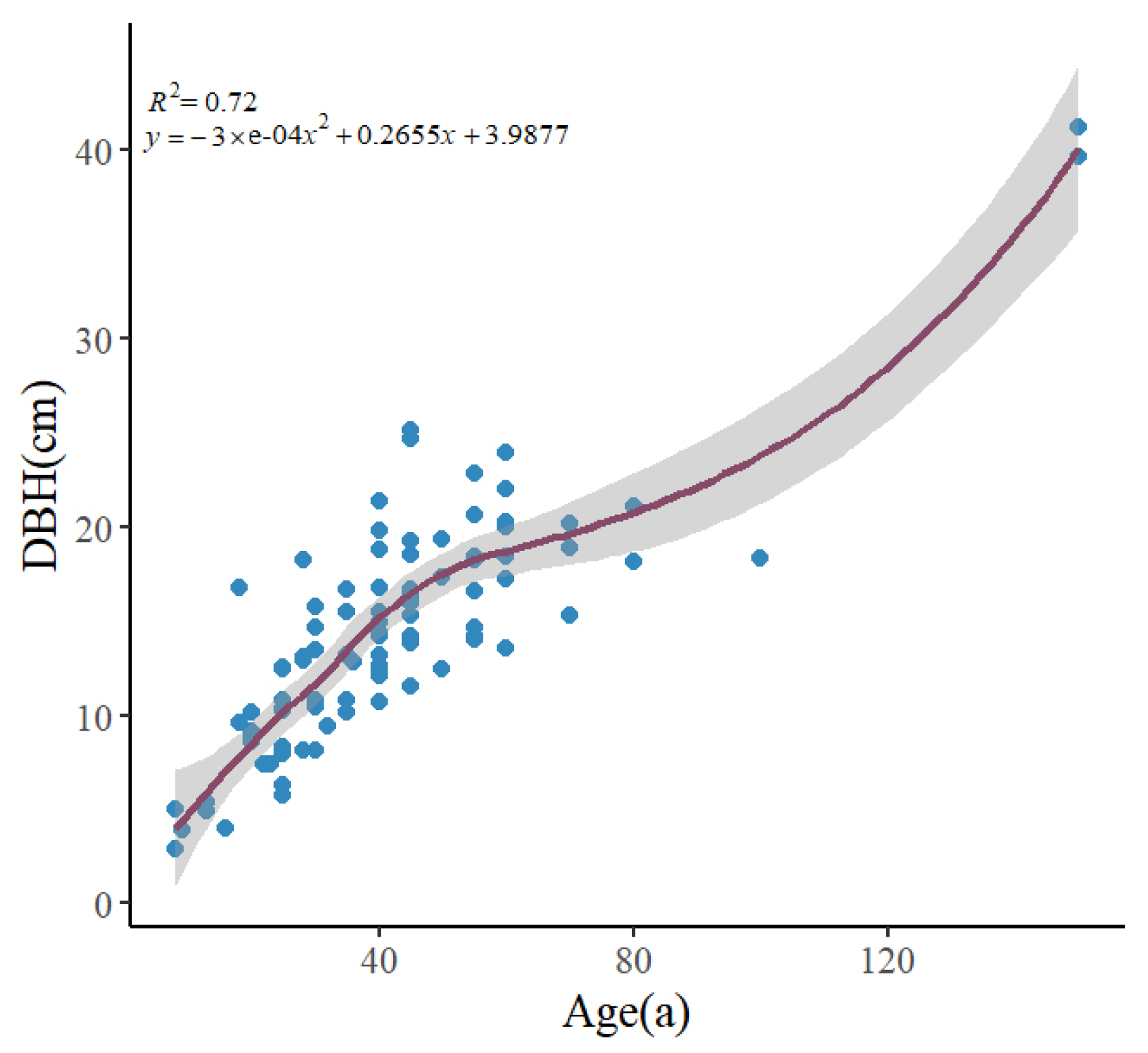
Dg (cm)	2.854	41.272	14.486	6.405	3.990	24.722	14.581	5.611
Hm (m)	2.200	24.296	10.610	4.453	2.821	15.515	10.178	3.490
Vw (m3 ha−1)	1.058	719.049	259.727	168.406	19.031	701.766	251.792	171.119

, and the basic form of model fitting is shown in Equation (12).

$$W_i=a\cdot {D_g}^b\cdot {H_m}^c$$

(12)

where W_i is the biomass, BCEF, and BEF of forest stands of each component, and R_i (R_ra, R_bw, R_fb, R_cs, and ρ) of forest stands; a, b, and c are the parameters (each component has the specific a, b, and c parameters).

2.4. Biomass and Biomass Factor Compatibility Model

During the growth of trees, the proportions of their biomass allocated to different components constantly change, exhibiting a relative growth relationship. There is also a certain regularity in the biomass distribution among different components. Therefore, stable biomass proportion relationships among various components can be established based on easily obtainable data and can then be used to estimate the biomass of other components. A compatibility model system has been constructed based on the relative growth relationship and algebraic sum relationship of trees. Considering the additivity condition, compatibility formulas for each component’s biomass and the total biomass were derived based on the algebraic sum of the biomass. The algebraic and relational expressions for the growing relationship between the biomass of each component and the total biomass of the tree are shown in Equations (13)–(16):

$${\mathrm{B}}_{\mathrm{t}}=B_a+B_r$$

(13)

$${\mathrm{B}}_{\mathrm{a}}=B_c+B_s$$

(14)

$$B_c=B_{br}+B_f$$

(15)

$$B_s=B_W+B_b$$

(16)

The wood biomass and the stable proportional relationships (R_ra, R_cs, R_bw, and R_fb) among the easily accessible data components were used to derive compatible biomass equations for each component. For instance, the calculation of branch biomass is intricately linked to leaf biomass. Considering that leaf biomass constitutes the difference between crown biomass and branch biomass, and also recognizing that leaf biomass is equivalent to branch biomass scaled by the ratio of branch to leaf biomass (R_fb), we can establish a compatibility equation for branch biomass. Similarly, bark biomass is defined as the difference between stem biomass and wood biomass. Additionally, bark biomass can be expressed as wood biomass multiplied by the ratio of wood to bark biomass (R_bw). From this, we infer that bark biomass equals wood biomass scaled by R_bw. Utilizing analogous reasoning, we formulated additivity equations for the biomass of other components, as detailed in Equations (17)–(23).

$$B_b=B_w\cdot R_{bw}$$

(17)

$$B_s=B_{{}_w}\cdot \left(1+R_{bw}\right)$$

(18)

$$B_{br}=\frac{B_w\cdot \left(1+R_{bw}\right)\cdot R_{cs}}{\left(1+R_{fb}\right)}$$

(19)

$$B_f=\frac{B_w\cdot \left(1+R_{bw}\right)\cdot R_{cs}\cdot R_{fb}}{\left(1+R_{fb}\right)}$$

(20)

$$B_c=B_{br}+B_f=B_w\cdot \left(1+R_{bw}\right)\cdot R_{cs}$$

(21)

$$B_a=B_c+B_s=B_w\cdot \left(1+R_{bw}\right)\cdot \left(1+R_{cs}\right)$$

(22)

$$B_t=B_a+B_r=B_w\cdot \left(1+R_{bw}\right)\cdot \left(1+R_{cs}\right)\cdot \left(1+R_{ra}\right)$$

(23)

The compatibility formulas for the BEF of each component were derived according to the definition of BEF, using the biomass relationship and combined with the above equation of biomass compatibility of each component. This is shown in Equations (24)–(31):

$$BE{F}_c=\frac{B_c}{B_s}=R_{cs}$$

(24)

$$BE{F}_b=\frac{B_b}{B_s}=\frac{R_{bw}}{\left(1+R_{bw}\right)}$$

(25)

$$BE{F}_w=\frac{B_w}{B_s}=\frac{1}{\left(1+R_{bw}\right)}$$

(26)

$$BE{F}_{br}=\frac{B_{br}}{B_s}=\frac{R_{cs}}{\left(1+R_{fb}\right)}$$

(27)

$$BE{F}_f=\frac{B_f}{B_s}=\frac{R_{cs}\cdot R_{fb}}{\left(1+R_{fb}\right)}$$

(28)

$$BE{F}_a=\frac{B_a}{B_s}=1+R_{cs}$$

(29)

$$BE{F}_r=\frac{B_r}{B_s}=R_{ra}\cdot \left(1+R_{cs}\right)$$

(30)

$$BE{F}_t=\frac{B_t}{B_s}=\left(1+R_{cs}\right)\cdot \left(1+R_{ra}\right)$$

(31)

Adhering to the definition of BCEF, combining the compatibility biomass equation of each component and the ρ factor, we derive the compatibility BCEF equations for each component. The compatibility equations of BCEF are shown in (32) to (39):

$$BCE{F}_w=\frac{B_w}{V_w}=\rho$$

(32)

$$BCE{F}_c=\frac{B_w\cdot \left(1+R_{bw}\right)\cdot R_{cs}}{V_w}=\rho \cdot \left(1+R_{bw}\right)\cdot R_{cs}$$

(33)

$$BCE{F}_b=\frac{B_w\cdot R_{bw}}{V_w}=\rho \cdot R_{bw}$$

(34)

$$BCE{F}_{br}=\frac{B_w\cdot \left(1+R_{bw}\right)\cdot R_{cs}}{V_w\cdot \left(1+R_{fb}\right)}=\rho \cdot \frac{\left(1+R_{bw}\right)\cdot R_{cs}}{\left(1+R_{fb}\right)}$$

(35)

$$BCE{F}_f=\frac{B_w\cdot \left(1+R_{bw}\right)\cdot R_{cs}\cdot R_{fb}}{V_w\cdot \left(1+R_{fb}\right)}=\rho \cdot \frac{\left(1+R_{bw}\right)\cdot R_{cs}\cdot R_{fb}}{\left(1+R_{fb}\right)}$$

(36)

$$BCE{F}_a=\frac{B_w\cdot \left(1+R_{bw}\right)\cdot \left(1+R_{cs}\right)}{V_w}=\rho \cdot \left(1+R_{bw}\right)\cdot \left(1+R_{cs}\right)$$

(37)

$$BCE{F}_r=\frac{B_w\cdot \left(1+R_{bw}\right)\cdot \left(1+R_{cs}\right)\cdot R_{ra}}{V_w}=\rho \cdot \left(1+R_{bw}\right)\cdot \left(1+R_{cs}\right)\cdot R_{ra}$$

(38)

$$BCE{F}_t=\frac{B_w\cdot \left(1+R_{bw}\right)\cdot \left(1+R_{cs}\right)\cdot \left(1+R_{ra}\right)}{V_w}=\rho \cdot \left(1+R_{bw}\right)\cdot \left(1+R_{cs}\right)\cdot \left(1+R_{ra}\right)$$

(39)

The biomass, BEF, and BCEF values were calculated according to the biomass compatibility models, BEF compatibility models, and BCEF compatibility models by introducing the R_i obtained from independent models. The calculated biomass values of each component are added to verify whether they are equal to the values calculated by the total biomass compatibility model.

2.5. Model Evaluation and Validation

The coefficient of determination (R²) and the mean square error (MSE) were used to validate model fit and performance [32]. The performance of the model was evaluated using four statistical metrics: relative error (RE), mean relative error (MRE), mean absolute error (MAE), and prediction accuracy (P). The calculations for these indicators are provided in Equations (40)–(43).

$$RE=\frac{{\displaystyle \sum y_i-{\displaystyle \sum {\widehat{y}}_i}}}{{\displaystyle \sum {\widehat{y}}_i}}\times 100\%$$

(40)

$$MRE=\frac{1}{N}\sum (\frac{y_i-{\widehat{y}}_i}{{\widehat{y}}_i})\times 100\%$$

(41)

$$MAE=\frac{1}{N}{\displaystyle \sum |\frac{y_i-{\widehat{y}}_i}{{\widehat{y}}_i}}|\times 100\%$$

(42)

$$P=\left[1-\frac{t_a\sqrt{{\displaystyle \sum {\left(y_i-{\widehat{y}}_i\right)}^2}}}{\widehat{\overline{y}}\sqrt{N\left(N-T\right)}}\right]\times 100\%$$

(43)

where y_i is true values; ${\widehat{y}}_i$ is estimated values; ${\widehat{\overline{y}}}_i$ is mean of estimated values; t_a is the t-distribution value at a confidence level of α = 0.05 depending on the degrees of freedom; N is the sample size of the test sample; T is the number of parameters in the model.

3. Results

3.1. Biomass Models for Pinus Densata Forest

As shown in

Table 3. The fitting results of the allometric biomass model for components of Pinus densata forest.

Components	Number of Samples	Model Parameter Estimates			R2	MSE
		a	b	c
Bw	79	6.1035	−0.9211	2.1432	0.7476	827.7531
Bb	79	0.8630	0.2662	0.8188	0.6106	22.2806
Bs	79	6.9594	−0.7781	1.9851	0.7372	1072.9630
Bbr	79	15.4272	−0.4155	0.8331	0.3382	137.6777
Bf	79	2.8332	−0.1242	0.5168	0.1603	9.2828
Bc	79	18.2257	−0.3665	0.7808	0.3207	199.0442
Ba	79	18.0495	−0.6584	1.6106	0.6649	2067.4490
Br	79	2.1598	−0.2416	1.0116	0.4684	23.3764
Bt	79	20.2150	−0.6259	1.5621	0.6540	2482.2650

, the various binary component biomass models were constructed using the D_g and H_m of the stand as independent variables. B_w had the best fit, with an R² value of 0.7476. B_f was the worst, with an R² of only 0.1603. The B_br and B_c models were also poor, with R² values of 0.3382 and 0.3207, respectively. B_f had the smallest MSE (9.2828).

As shown in

Table 4. The test results of the allometric biomass model for Pinus densata forest.

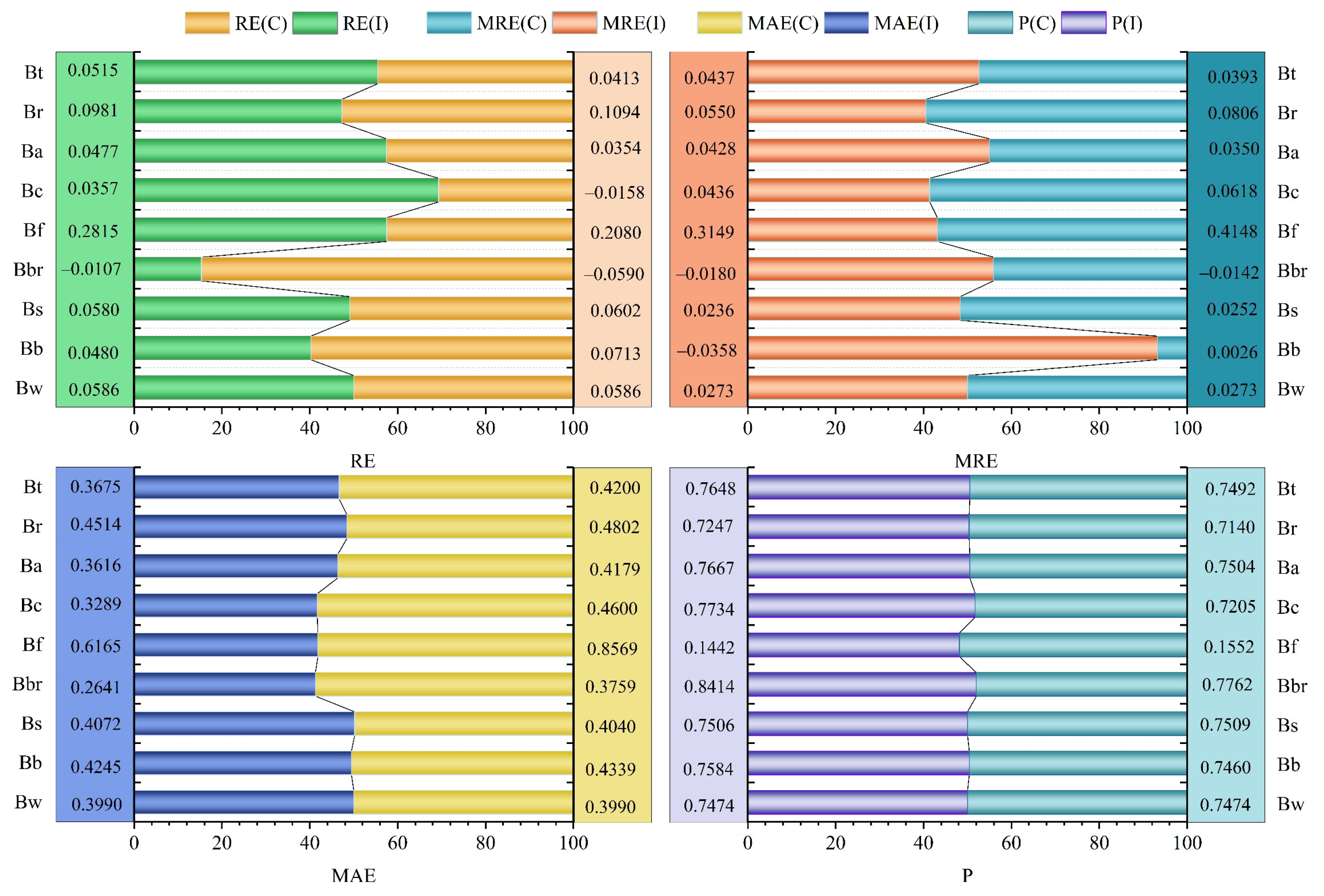
Components	RE	MRE	MAE	p
Bw	0.0586	0.0273	0.3990	0.7474
Bb	0.0713	0.0026	0.4339	0.7460
Bs	0.0602	0.0252	0.4040	0.7509
Bbr	−0.0590	−0.0142	0.3759	0.7762
Bf	0.2080	0.4148	0.8569	0.1552
Bc	−0.0158	0.0618	0.4600	0.7205
Ba	0.0354	0.0350	0.4179	0.7504
Br	0.1094	0.0806	0.4802	0.7140
Bt	0.0413	0.0393	0.4200	0.7492

, the RE ranged from −0.059 to 0.208, the MRE ranged from −0.014 to 0.4148, the MAE ranged from 0.37 to 0.85, and the p value ranged from 0.1552 to 0.776. The B_br model had the highest p value (0.7762), while the B_f model had the lowest p value (0.1552). The p values for the other biomass components were all above 0.71.

3.2. BEF Models for Pinus Densata Forest

As shown in

Table 5. The fitting results of the parameter for various components of Pinus densata forest.

Components	Number of Samples	Model Parameter Estimates			R2	MSE
		a	b	c
BEFw	79	0.9173	−0.1492	0.1474	0.6538	0.0003
BEFb	79	0.0927	0.9490	−0.9456	0.6412	0.0003
BEFbr	79	7.6920	−0.1331	−1.1075	0.9944	0.0012
BEFf	79	2.2482	−0.0423	−1.4085	0.9711	0.0004
BEFc	79	9.8850	−0.1190	−1.1590	0.9928	0.0024
BEFa	79	6.8847	−0.1497	−0.4803	0.9382	0.0202
BEFr	79	0.2837	0.5112	−0.9008	0.7026	0.0006
BEFt	79	7.0382	−0.0947	−0.5152	0.9423	0.0211

, the independent model based on the allometric equation provided a good performance for the BEF of various components. All models had a good fit, with R² ranging from 0.54 to 0.99; BEF_br had the largest R² and BEF_b had the smallest R². All BEF models had lower MSE values, ranging from 0.0003 to 0.0211. BEF_w and BEF_b had the smallest MSE (0.0003) and BEF_t had the largest MSE (0.0211).

As shown in

Table 6. The test results of Pinus densata BEF.

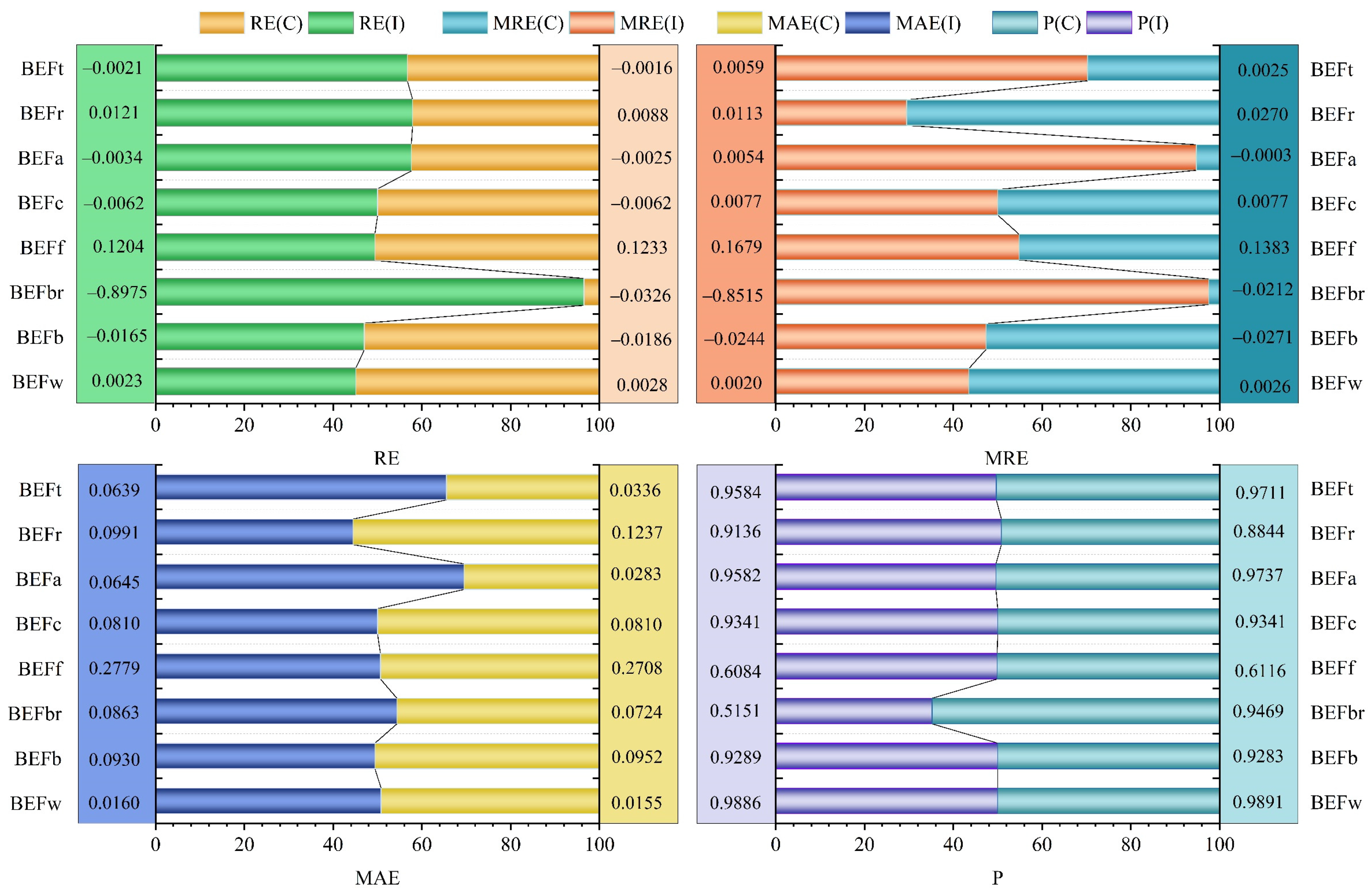
Components	RE	MRE	MAE	p
BEFw	0.0023	0.0020	0.0160	0.9886
BEFb	−0.0165	−0.0244	0.0930	0.9289
BEFbr	−0.8975	−0.8515	0.0863	0.5151
BEFf	0.1204	0.1679	0.2779	0.6084
BEFc	−0.0062	0.0077	0.0810	0.9341
BEFa	−0.0034	0.0054	0.0645	0.9582
BEFr	0.0121	0.0113	0.0991	0.9136
BEFt	−0.0021	0.0059	0.0639	0.9584

, the independent BEF models were evaluated using RE, which ranged from −0.8975 to 0.1204. The largest RE value was BEF_br (−0.8975), whereas the smallest was BEF_t (−0.0021). There was a relatively larger difference between the predicted values and actual values of BEF_br, as its MRE value (−0.8515) was the greatest. On the other hand, BEF_w had a higher predictive accuracy because its MRE value was the smallest (0.0020). Similarly, BEF_w had the smallest MAE value of 0.0160, indicating a relatively lower predictive error. On the contrary, BEF_f had the largest MAE value (0.2779). The p values of the BEF models ranged from 0.5151 to 0.9886, with BEF_br and BEF_w having the lowest and highest values, respectively.

In summary, the BEF models for each component exhibited varying levels of goodness of fit and predictive capability.

3.3. BCEF Models for Pinus Densata Forest

As shown in

Table 7. The fitting results of the allometric BCEF model for the components of Pinus densata forest.

Components	Number of Samples	Model Parameter Estimates			R2	MSE
		a	b	c
BCEFw	79	0.4462	−0.3730	0.2952	0.8700	0.0001
BCEFb	79	0.0446	0.7400	−0.8104	0.5511	0.0000
BCEFs	79	0.4862	−0.2233	0.1474	0.8298	0.0001
BCEFbr	79	3.8870	−0.3726	−0.9618	0.9945	0.0002
BCEFf	79	1.1394	−0.2769	−1.2718	0.9785	0.0001
BCEFc	79	4.9988	−0.3576	−1.0146	0.9936	0.0004
BCEFa	79	3.5430	−0.3987	−0.3317	0.9435	0.0036
BCEFr	79	0.1380	0.2986	−0.7665	0.7501	0.0001
BCEFt	79	3.6139	−0.3423	−0.3668	0.9468	0.0038

, the independent BCEF_br model had the largest R² (0.9944) and the BCEF_b model had the smallest R² (0.5511). The MSE values of most models were small; the BCEF_b model had the smallest MSE, with a value of 0, and the BCEF_t model had the largest MSE, with a value of 0.0038.

As shown in

Table 8. Test results of Pinus densata BCEF.

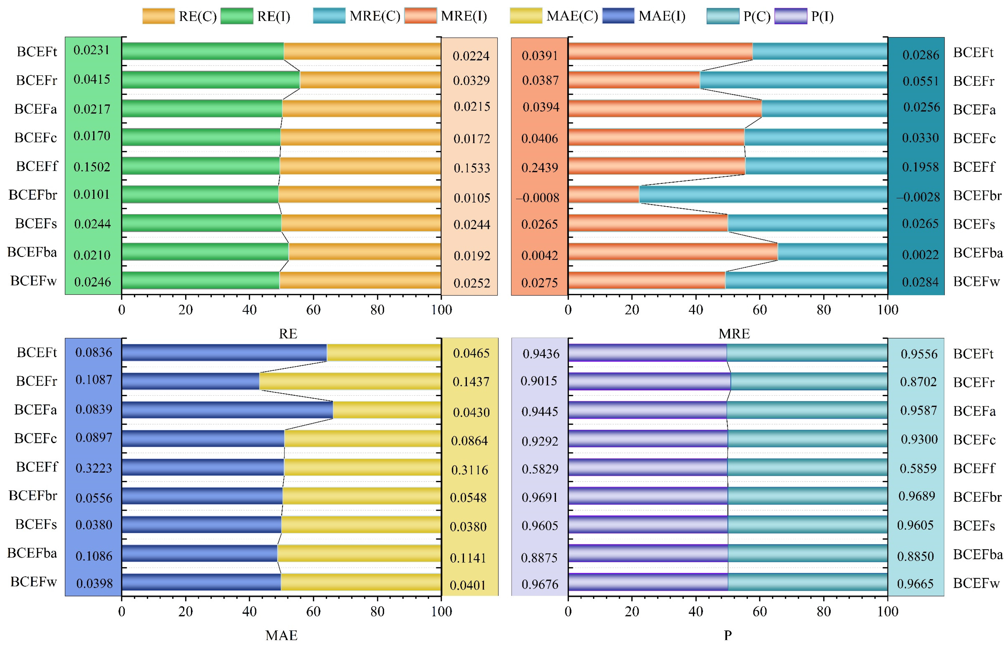
Components	RE	MRE	MAE	p
BCEFw	0.0246	0.0275	0.0398	0.9676
BCEFb	0.0210	0.0042	0.1086	0.8875
BCEFs	0.0244	0.0265	0.0380	0.9605
BCEFbr	−0.0101	−0.0008	0.0556	0.9691
BCEFf	0.1502	0.2439	0.3223	0.5829
BCEFc	0.0170	0.0406	0.0897	0.9292
BCEFa	0.0217	0.0394	0.0839	0.9445
BCEFr	0.0415	0.0387	0.1087	0.9015
BCEFt	0.0231	0.0391	0.0836	0.9436

, the RE values were uniformly small for the BCEF models, ranging from −0.0101 to 0.1202. The RE value of the BCEF_br model was the smallest, and the BCEF_f model had the largest RE value. Correspondingly, BCEF_br and BCEF_f also had the smallest (0.0008) and largest (0.2439) MRE, respectively. Moreover, BCEF_s had the smallest MAE, with a value of 0.038, and BCEF_f had the largest MAE (0.3223). BCEF_br had the largest p value (0.9691) and BCEF_f had the smallest p value (0.5829). The p values of the other models ranged from 0.8875 to 0.9676.

In summary, the BCEF_br model had the highest P and R², meaning that it had the best predictive accuracy. The RE and MSE of the BCEF_f model were larger, indicating its worse prediction accuracy. Overall, all independent BCEF models can provide relatively accurate estimations for Pinus densata forests.

3.4. The Models of Rra, Rcs, Rbw, Rfb, and ρ

The goodness of fit for the independent R_ra, R_cs, R_bw, R_fb, and ρ models are shown in

Table 9. The fitting results of R_ra, R_cs, R_bw, R_fb, and ρ models for components of Pinus densata forest.

Components	Number of Samples	Model Parameter Estimates			R2	MSE
		a	b	c
Rra	79	0.0654	0.4656	−0.4078	0.1417	0.0003
Rcs	79	9.8850	−0.1190	−1.1590	0.9928	0.0024
Rfb	79	0.2494	0.1625	−0.3014	0.1122	0.0021
Rbw	79	0.1013	1.0878	−1.0806	0.6125	0.0006
ρ	79	0.4862	−0.2233	0.1474	0.8298	0.0001

. The R² values ranged from 0.1122 to 0.9928, indicating an overall good fit of the models. The MSE values were consistently small, ranging from 0.0001 to 0.0024, further confirming the good fit of the models.

As shown in

Table 10. The test results of R_ra, R_cs, R_bw, R_fb, and ρ for Pinus densata.

Components	RE	MRE	MAE	p
Rra	0.0345	0.0269	0.1166	0.8930
Rcs	−0.0062	0.0077	0.0810	0.9341
Rfb	0.2559	0.2273	0.3426	0.2964
Rbw	−0.0144	−0.0266	0.1116	0.9098
ρ	0.0244	0.0265	0.0380	0.9605

, the RE values for each model were relatively low, with the largest RE value being 0.2559 and the smallest being −0.0062. The MRE values were all less than 0.2273, and all MAE values were less than 0.3426. These results show that the independent R_ra, R_cs, R_bw, R_fb, and ρ models had low prediction errors. Moreover, the independent R_fb model had an especially small p value (0.2964), whereas the p values for the other models ranged from 0.8930 to 0.9605.

The results have shown that it was feasible to build an independent model using Dg and Hm and to calculate ratios (R_ra, R_cs, R_bw, R_fb, and ρ) from that independent model. These ratios will subsequently be used to calculate the compatibility model.

3.5. Comparison of Independent Models and Compatibility Models

The independence test results for the independent and the compatible models are compared in Figure 2. The independent models generally had higher RE values than the compatibility models. Most of the models exhibited similar MRE values for both the independent model and compatibility model, with the largest MRE value being below 0.42. The largest difference in MRE values was observed for the B_f model; the MRE value of the independent B_f model was 0.1001, which was less than that of the compatible B_f model. The compatible models generally had slightly higher MAE values than the independent biomass models, with the largest difference observed for the B_f model. This indicated that the computational errors of these models were generally small. Both types of biomass models were very close in terms of p values and were generally above 0.7, indicating that these biomass models provided accurate predictions overall.

3.6. Comparison of the BEF of the Compatibility Models and Independent Models

As shown in Figure 3, the RE values of the two type models for the same components were close, but there was a significant difference in the MRE value of the B_br model. This indicates that the compatible model prediction error of the B_br was smaller than that of the independent B_br model. The independent BEF model generally had slightly higher MRE values than the BEF of the compatible model. The difference in MAE values between the two type models was small; the BEF_f model exhibited the largest error, with a maximum absolute average relative error of 0.3.

The p value analysis showed that the p values were higher than 0.8 for all models in this study except for the BEF_f model. This analysis indicated that most BEF models had high estimation accuracy and that the compatible models generally had smaller errors and higher accuracy compared to the independent models.

Overall, the compatible models for BEF in Pinus densata stands had smaller errors and higher forecast accuracy compared to the independent models. The compatibility models can improve the p values of BEF_w, BEF_br, BEF_f, BEF_a, and BEF_t, especially for the BEF_br.

3.7. Comparison of the BCEF of the Independent Models and Compatibility Models

As shown in Figure 4, the MRE and MAE values indicate that both the independent BCEF model and the BCEF compatibility model exhibited small errors. Most of the BCEF models had p values above 0.8, except for the BCEF_f model.

4. Discussion

4.1. The Performance of Compatibility Models

Our study showed that independent and compatible models can be used not only for the total biomass estimation but also for each component’s biomass. Since the estimations for all components and total biomass showed no significant difference between the two models, the results are consistent with the findings of Atticus [33]. In this study, the overall accuracy estimation for the two models was greater than 0.7, which coincides with the results of Xin’s study [34]. However, this value was lower than Tang’s result [12], since the root biomass was added to the total biomass in our study. The foliage biomass model exhibited relatively lower accuracy, with a value of 0.15. This may have been caused by B_f loss during the data collection. Scale dependency, spatial heterogeneity, and model error may also have impacted the estimation results [35,36]. The current findings also indicated that the compatibility model can obtain better estimation accuracy. However, the independent model did not comply with the compatibility condition, namely that the sum of the biomass of all components is equal to the total biomass. Hence, the compatible model was applied to infer the conversion coefficient.

4.2. The Model Performance of the BEF and BCEF

The mean p values of BEF and BCEF for the total, branch, wood, and bark were all ≥0.90, except for the foliage, which had the lowest p values (BEF_f = 0.61, BCEF_f = 0.59). Our results aligned with those of Schepaschenko et al. [37], and the values of BEF and BCEF obtained were all within the range of those that provided by the IPCC. For example, our result of the mean value of the BEF was 1.6, whereas the mean IPCC BEF value is 1.3. The range of BEF for each component was 1.4 to 2.1, which is similar to the IPCC’s BEF range of 1.15 to 3.2 [10]. While the mean value of BCEF from the IPCC is 0.7, our result was 0.61. The range of BCEF in our study was 0.44–0.89, which was within IPCC’s range of 0.4–1.0. However, the BEF and BCEF values provided by the IPCC are permanent. The latest IPCC data was published in 2006 [38], meaning that they have not been changed for a long time. Furthermore, their data did not include all species and was a relatively rough calculation of continental and global ecozones. Studies [38,39,40,41] have indicated that the values of BEF and BCEF vary under different conditions. Therefore, the values from the IPCC cannot accurately represent the real situation of a research region [42,43,44], especially an area with high forest heterogeneity. Jalkanen et al. [45] also demonstrated that forest biomass was easily underestimated when using the BEF and BCEF provided by IPCC, illustrating that the conversion coefficient provided by the IPCC was inapplicable to some extent. Our research supplied a series of models that could calculate BEF, BCEF, and forest biomass using relevant ratios, providing an alternative to the single top-down method of deriving the biomass. Besides, remote sensing techniques are widely used to exact the forest information due to the merit of being highly efficient and non-destructive [46]. Hence, ratio factors that can be obtained from remote sensing, such as the crown and stem, can be used to quickly and easily calculate the BEF and BCEF of different components for various forest species. This method can be used to efficiently and accurately calculate the biomass in stands at large scales. This study effectively compensates for the disadvantages of IPCC data.

4.3. Applicability and Limitations

The foliage biomass accuracy was much lower compared with the other components, which reduced the applicability of the foliage model. The reason for this lower accuracy needs to be clarified, and a feasible method for improving the foliage biomass accuracy needs to be explored [47]. Furthermore, biomass accumulation is directly correlated with the age of the trees, but the study did not add the stand age into the model, since the age showed a high positive relationship with DHB (Figure 5). Additionally, the basic model was calibrated using DBH and H. However, forest growth is limited by many factors, such as the density, competition environment, stand condition, and disturbance degree. Thus, additional factors such as the spatial structure index, the angle index, neighborhood comparison, forest layer index, and degree of openness could be taken into account when building future mixed-effects models for the forest stand level to enhance the estimation accuracy.

5. Conclusions

Deducting reliable and high-accuracy models is essential to estimating forest biomass for large regions, both above and below ground, when there is insufficient survey data. In this study, 98 sample plots were used to build a basic model according to allometric equations, and the component biomass values and ratios were calculated. The independent model was compared with the compatibility model. The results were as follows:

(1)

The compatible biomass models were constructed to explore whether they could handle the compatibility problem between the total biomass and the biomass of different components. The results showed that the summation of each component’s biomass was equal to the total biomass.

(2)

The estimation accuracy of the compatible models was similar to that of the independent biomass models. Excepting the B_f model, which had a relatively lower accuracy, the accuracy for all of the component models was greater than 0.7. The accuracy was slightly lower than in other studies because the root biomass was added into the total biomass, which decreased the accuracy of the total biomass estimation.

(3)

The total error of BEF and BCEF models for most components was less than 0.1 and the estimation accuracy was higher than 0.87, indicating that reliable biomass estimations can be calculated using the corresponding conversion coefficient for the tree species in a specific region. The AGB and UGB of the forest can be accurately estimated by applying these compatible models or biomass factors (BEF, BCEF).

(4)

Although all ratios (R_ra, R_cs, R_bw, R_fb, and ρ) can be used to calculate the BEF and BCEF, the R_cs was the most stable and easy to measure, and it was a unique ratio that could be used to infer all the other models. At the same time, the other ratios need to be composed to deduce all models.

References

- De Wit, H.A.; Palosuo, T.; Hylen, G.; Liski, J. A carbon budget of forest biomass and soils in southeast Norway calculated using a widely applicable method. For. Ecol. Manag. 2006, 225, 15–26. [Google Scholar] [CrossRef]
- Kurniawan, K.; Supriatna, J.; Sapoheluwakan, J.; Soesilo, T.E.B.; Mariati, S.; Gunarso, G. The analysis of forest and land fire and carbon and greenhouse gas emissions on the climate change in Indonesia. Agbioforum 2022, 24, 1–11. [Google Scholar]
- Sileshi, G.W. A critical review of forest biomass estimation models, common mistakes and corrective measures. For. Ecol. Manag. 2014, 329, 237–254. [Google Scholar] [CrossRef]
- Wu, H.; Xu, H. A review of sampling and modeling techniques for forest biomass inventory. Agric. Rural. Stud. 2023, 1, ar01010002. [Google Scholar] [CrossRef]
- Lehtonen, A.; Mäkipää, R.; Heikkinen, J.; Sievänen, R.; Liski, J. Biomass expansion factors (BEFs) for Scots pine, Norway spruce and birch according to stand age for boreal forests. For. Ecol. Manag. 2004, 188, 211–224. [Google Scholar] [CrossRef]
- Ameztegui, A.; Rodrigues, M.; Granda, V. Uncertainty of biomass stocks in Spanish forests: A comprehensive comparison of allometric equations. Eur. J. For. Res. 2022, 141, 395–407. [Google Scholar] [CrossRef]
- Ali, H.; Mohammadi, J.; Shataee Jouibary, S. Allometric Models and Biomass Conversion and Expansion Factors to Predict Total Tree-level Aboveground Biomass for Three Conifers Species in Iran. For. Sci. 2023, 69, fxad013. [Google Scholar] [CrossRef]
- Teobaldelli, M.; Somogyi, Z.; Migliavacca, M.; Usoltsev, V.A. Generalized functions of biomass expansion factors for conifers and broadleaved by stand age, growing stock and site index. For. Ecol. Manag. 2009, 257, 1004–1013. [Google Scholar] [CrossRef]
- Ochał, W.; Wertz, B.; Orzeł, S. Above-ground biomass allocation and potential carbon sink of black pine—A case study from southern Poland. Ann. For. Res. 2022, 65, 71–90. [Google Scholar] [CrossRef]
- Eggleston, H.; Buendia, L.; Miwa, K.; Ngara, T.; Tanabe, K. 2006 IPCC Guidelines for National Greenhouse Gas Inventories; Institute for Global Environmental Strategies: Hayama, Japan, 2006. [Google Scholar]
- Güner, Ş.T.; Diamantopoulou, M.J.; Poudel, K.P.; Çömez, A.; Özçelik, R. Employing artificial neural network for effective biomass prediction: An alternative approach. Comput. Electron. Agric. 2022, 192, 106596. [Google Scholar] [CrossRef]
- Tang, S.; Zhang, H.; Xu, H. Study on establish and estimate method of compatible biomass model. Sci. Silvae Sin. 2000, 18, 19–27. [Google Scholar] [CrossRef]
- Xie, L.; Wang, T.; Miao, Z.; Hao, Y.; Dong, L.; Li, F. Considering random effects and sampling strategies improves individual compatible biomass models for mixed plantations of Larix olgensis and Fraxinus mandshurica in northeastern China. For. Ecol. Manag. 2023, 537, 120934. [Google Scholar] [CrossRef]
- Parresol, B.R. Assessing tree and stand biomass: A review with examples and critical comparisons. For. Sci. 1999, 45, 573–593. [Google Scholar]
- Parresol, B.R. Additivity of nonlinear biomass equations. Can. J. For. Res. 2001, 31, 865–878. [Google Scholar] [CrossRef]
- Affleck, D.L.; Diéguez-Aranda, U. Additive nonlinear biomass equations: A likelihood-based approach. For. Sci. 2016, 62, 129–140. [Google Scholar] [CrossRef]
- Zhang, C.; Peng, D.-L.; Huang, G.-S.; Zeng, W.-S. Developing aboveground biomass equations both compatible with tree volume equations and additive systems for single-trees in poplar plantations in Jiangsu Province, China. Forests 2016, 7, 32. [Google Scholar] [CrossRef]
- Zhao, D.; Westfall, J.; Coulston, J.W.; Lynch, T.B.; Bullock, B.P.; Montes, C.R. Additive biomass equations for slash pine trees: Comparing three modeling approaches. Can. J. For. Res. 2019, 49, 27–40. [Google Scholar] [CrossRef]
- Robinson, D. Implications of a large global root biomass for carbon sink estimates and for soil carbon dynamics. Proc. Royal Soc. B 2007, 274, 2753–2759. [Google Scholar] [CrossRef]
- Luo, W.; Lan, R.; Chen, D.; Zhang, B.; Xi, N.; Li, Y.; Fang, S.; Valverde-Barrantes, O.J.; Eissenstat, D.M.; Chu, C. Limiting similarity shapes the functional and phylogenetic structure of root neighborhoods in a subtropical forest. New Phytol. 2021, 229, 1078–1090. [Google Scholar] [CrossRef]
- Yu, X.; Ge, H.; Lu, D.; Zhang, M.; Lai, Z.; Yao, R. Comparative study on variable selection approaches in establishment of remote sensing model for forest biomass estimation. Remote Sens. 2019, 11, 1437. [Google Scholar] [CrossRef]
- Clough, B.; Dixon, P.; Dalhaus, O. Allometric relationships for estimating biomass in multi-stemmed mangrove trees. Aust. J. Bot. 1997, 45, 1023–1031. [Google Scholar] [CrossRef]
- Wang, C. Biomass allometric equations for 10 co-occurring tree species in Chinese temperate forests. For. Ecol. Manag. 2006, 222, 9–16. [Google Scholar] [CrossRef]
- Vorster, A.G.; Evangelista, P.H.; Stovall, A.E.; Ex, S. Variability and uncertainty in forest biomass estimates from the tree to landscape scale: The role of allometric equations. Carbon Balance Manag. 2020, 15, 1–20. [Google Scholar] [CrossRef]
- Puletti, N.; Grotti, M.; Ferrara, C.; Chianucci, F. Lidar-based estimates of aboveground biomass through ground, aerial, and satellite observation: A case study in a Mediterranean forest. J. Appl. Remote Sens. 2020, 14, 044501. [Google Scholar] [CrossRef]
- Chianucci, F.; Puletti, N.; Grotti, M.; Ferrara, C.; Giorcelli, A.; Coaloa, D.; Tattoni, C. Nondestructive Tree Stem and Crown Volume Allometry in Hybrid Poplar Plantations Derived from Terrestrial Laser Scanning. For. Sci. 2020, 66, 737–746. [Google Scholar] [CrossRef]
- Zhang, J.; Lu, C.; Xu, H.; Wang, G. Estimating aboveground biomass of Pinus densata-dominated forests using Landsat time series and permanent sample plot data. J. For. Res. 2019, 30, 1689–1706. [Google Scholar] [CrossRef]
- Li, C.; Chen, D.; Wu, D.; Su, X. Design of an EIoT system for nature reserves: A case study in Shangri-La County, Yunnan Province, China. Int. J. Sustain. Dev. World Ecol. 2015, 22, 184–188. [Google Scholar] [CrossRef]
- Ma, F.; Zhao, C.; Milne, R.; Ji, M.; Chen, L.; Liu, J. Enhanced drought-tolerance in the homoploid hybrid species Pinus densata: Implication for its habitat divergence from two progenitors. New Phytol. 2010, 185, 204–216. [Google Scholar] [CrossRef]
- Wang, B.; Mao, J.; Gao, J.; ZHao, W.; Wang, X. Colonization of the Tibetan Plateau by the homoploid hybrid pine Pinus densata. Mol. Ecol. 2011, 20, 3796–3811. [Google Scholar] [CrossRef]
- Ou, G.; Li, C.; Lv, Y.; Wei, A.; Xiong, H.; Xu, H.; Wang, G. Improving aboveground biomass estimation of Pinus densata forests in Yunnan using Landsat 8 imagery by incorporating age dummy variable and method comparison. Remote Sens. 2019, 11, 738. [Google Scholar] [CrossRef]
- Zeng, W.; Luo, Q.; He, D. Research on weighting regression and modelling. Sci. Silvae Sin. 1999, 35, 5–11. [Google Scholar]
- Stovall, A.E.L.; Vorster, A.; Anderson, R.; Evangelista, P. Developing nondestructive species-specific tree allometry with terrestrial laser scanning. Methods Ecol. Evol. 2023, 14, 280–290. [Google Scholar] [CrossRef]
- Xin, S.; Mahardika, S.B.; Jiang, L. Stand-level biomass estimation for Korean pine plantations based on four additive methods in Heilongjiang province, northeast China. Cerne 2022, 28, e103008. [Google Scholar] [CrossRef]
- Haboudane, D.; Miller, J.R.; Tremblay, N.; Zarco-Tejada, P.J.; Dextraze, L. Integrated narrow-band vegetation indices for prediction of crop chlorophyll content for application to precision agriculture. Remote Sens. Environ. 2002, 81, 416–426. [Google Scholar] [CrossRef]
- Fu, Y.; Lei, Y.; Zeng, W. Uncertainty Assessment in Regional-Scale Above Ground Biomass Estimation of Chinese Fir. Sci. Silvae Sin. 2014, 50, 79–86. [Google Scholar]
- Schepaschenko, D.; Moltchanova, E.; Shvidenko, A.; Blyshchyk, V.; Dmitriev, E.; Martynenko, O.; See, L.; Kraxner, F. Improved Estimates of Biomass Expansion Factors for Russian Forests. Forests 2018, 9, 312. [Google Scholar] [CrossRef]
- Langner, A.; Achard, F.; Grassi, G. Can recent pan-tropical biomass maps be used to derive alternative Tier 1 values for reporting REDD+ activities under UNFCCC? Environ. Res. Lett. 2014, 9, 124008. [Google Scholar] [CrossRef]
- Fang, J.-y.; Wang, G.G.; Liu, G.-h.; Xu, S.-l. Forest biomass of China: An estimate based on the biomass–volume relationship. Ecol. Appl. 1998, 8, 1084–1091. [Google Scholar] [CrossRef]
- Luo, Y.; Zhang, X.; Wang, X.; Ren, Y. Dissecting variation in biomass conversion factors across China’s forests: Implications for biomass and carbon accounting. PLoS ONE 2014, 9, e94777. [Google Scholar] [CrossRef]
- Jagodziński, A.M.; Dyderski, M.K.; Gęsikiewicz, K.; Horodecki, P.; Cysewska, A.; Wierczyńska, S.; Maciejczyk, K. How do tree stand parameters affect young Scots pine biomass?—Allometric equations and biomass conversion and expansion factors. For. Ecol. Manag. 2018, 409, 74–83. [Google Scholar] [CrossRef]
- Fang, J.; Chen, A.; Peng, C.; Zhao, S.; Ci, L. Changes in forest biomass carbon storage in China between 1949 and 1998. Science 2001, 292, 2320–2322. [Google Scholar] [CrossRef] [PubMed]
- Joosten, R.; Schumacher, J.; Wirth, C.; Schulte, A. Evaluating tree carbon predictions for beech (Fagus sylvatica L.) in western Germany. For. Ecol. Manag. 2004, 189, 87–96. [Google Scholar] [CrossRef]
- Haripriya, G. Estimates of biomass in Indian forests. Biomass Bioenergy 2000, 19, 245–258. [Google Scholar] [CrossRef]
- Jalkanen, A.; Mäkipää, R.; Ståhl, G.; Lehtonen, A.; Petersson, H. Estimation of the biomass stock of trees in Sweden: Comparison of biomass equations and age-dependent biomass expansion factors. Ann. For. Sci. 2005, 62, 845–851. [Google Scholar] [CrossRef]
- Sullivan, M.J.P.; Talbot, J.; Lewis, S.L.; Phillips, O.L.; Qie, L.; Begne, S.K.; Chave, J.; Cuni-Sanchez, A.; Hubau, W.; Lopez-Gonzalez, G.; et al. Diversity and carbon storage across the tropical forest biome. Sci. Rep. 2017, 7, 39102. [Google Scholar] [CrossRef]
- Zeng, W.; Zhang, L.; Chen, X.; Cheng, Z.; Ma, K.; Li, Z. Construction of compatible and additive individual-tree biomass models for Pinus tabulaeformis in China. Can. J. For. Res. 2017, 47, 467–475. [Google Scholar] [CrossRef]