A General Rule-Based Framework for Generating Alternatives for Forest Ecosystem Management Decision Support Systems

Abstract

Linear programming formulations of forest ecosystem management (FEM) problems proposed in the 1960s have been adapted and improved upon over the years. Generating management alternatives for forest planning is a key step in building these models. Global forests are diverse, and a variety of models have been developed to simulate management alternatives. This paper describes iGen, a forest prescription generator that employs a rule-based system (AI-RBS), an AI technique that is often used for expert systems. iGen was designed with the goal of being able to generate management alternatives for virtually any FEM problem. The prescription generator is not designed for, adapted to, focused on—and ideally not limited to—any specific region, landscape, forest condition, projection method, or yield function. Instead, it aims to maximize generality, enabling it to address a broad range of FEM problems. The goal is that practitioners and researchers who do not have and do not want to develop their own alternative generator can use iGen as a prescription generator for their problem instances. For those who choose to develop their own alternative generators, we hope that the concepts and algorithms we propose in this paper will be useful in designing their own systems. iGen’s flexibility can be attributed to three key features. First, users can define the state variable vector for management units according to the available data, models (production functions), and objectives of their problem instance. Second, users also define the types of interventions that can be applied to each type of management unit and create a rule base describing the conditions under which each intervention can be applied. Finally, users specify the equations of motion that determine how the state vector for each management unit will be updated over time, depending on which, if any, interventions are applied. Other than this basic structure, virtually everything in an iGen problem instance is user-defined. iGen uses these key elements to simulate all possible management prescriptions for each management unit and stores the resulting information in a database that is structured to efficiently store the output data from these simulations and to facilitate the generation of optimization models for ultimately determining the Pareto frontier for a given FEM problem. This article introduces iGen, illustrating its concepts, structure, and algorithms through two FEM example problems with contrasting forest management practices: natural regeneration with shelterwood harvests and plantation/coppice. For data and iGen source programs, visit github.com/SilvanaNobre/iGenPaper.

1. Introduction

The forest ecosystem management (FEM) problem can be defined as characterizing the Pareto frontier for the problem of selecting a management prescription for the duration of some planning horizon for each forest management unit within a specified planning area, given a set of management and policy objectives and constraints. A management unit is defined here as either a contiguous area to be managed with a single prescription or as a collection of similar areas to which a common set of management prescriptions can be applied and for which the associated inputs and outputs for a given prescription will be sufficiently similar. While other approaches could be used to solve the FEM problem, this paper focuses on situations where the problem will be formulated as either a linear program (LP) or mixed-integer linear programming (MIP) problem [1]. To formulate this problem, one needs to have (1) a set of forest management units, (2) a set of management prescriptions for each unit, and (3) a set of management constraints and objectives. It is also necessary to quantify the contribution of each management alternative to each constraint or objective, i.e., the relevant inputs and outputs associated with each prescription for a given management unit [2]. For the purposes of this paper, we refer to any problem that fits this definition as a FEM problem. FEM problems are frequently quite complex, and considerable research has gone into the development of decision support systems to assist forest planners in finding efficient solutions to such problems [3,4,5,6,7,8,9].

A forest ecosystem management decision support system (FEMDSS) is a software system that facilitates the formulation, solution, storage, and interpretation of FEM models [3,6,8,10,11,12,13,14,15,16,17]. It must be able to project the state, including the associated inputs and outputs, of each management unit under each possible management prescription for the entire planning horizon. It must then be able to use the information generated about the projected states (and inputs and outputs) of each management unit to formulate and solve a set of optimization models, store the solutions of these models, and use the solution information to enable decision-makers to visualize and understand the attributes of the Pareto frontier and the implied tradeoffs among objectives. Therefore, the key tasks that a FEMDSS must accomplish are: (1) generate alternative management prescriptions for each management unit; (2) formulate one or more models to identify an optimal management prescription for each management unit, given various management objectives and constraints; (3) solve the optimization model(s) formulated in step 2; and (4) interpret the solution(s) to the management problem (Figure 1).

Most of the literature related to the FEMDSS problem has addressed questions related to the formulation (Step 2 in Figure 1) and solution (Step 3) of these optimization models [3,10,18,19,20,21,22,23,24,25,26] or to the problem of generating and/or visualizing the Pareto frontier for multi-objective problems (Step 4) [27,28,29]. This paper focuses on the alternative generation process within a general FEMDSS framework (Step 1). Since the 1960s, numerous forest management alternative generators have been developed [11,30,31,32]. To our knowledge, however, no one has developed an alternative generator for a FEMDSS that can be applied to any and all FEM problems. The perceived need for multiple generators arises due to the unique features of each FEM planning problem, which existing solutions often cannot handle [33]. Various FEM problems differ in the types of management regimes, outputs (e.g., wood, wildlife habitat, carbon storage), and production functions used to predict inputs and outputs for each management alternative. Growth and yield models, the most common production functions, vary widely, ranging from simple yield models [34,35] to more complex individual tree models [36,37] and process-based physiological models [38]. Moreover, models used in different regions frequently require different inputs (e.g., age, site class, basal area, forest type, tree list) and provide different output information (e.g., species mix, product mix to meet local market demand). Therefore, forest planners have felt the need to develop their own alternative generators tailored to their specific FEM problems.

According to Eriksson and Bergh [39], an effective stand simulator should be able to cover a broad problem domain and generate a range of management options for each stand so that preferred management strategies for each management unit can be assessed in the context of identifying an overall optimal strategy for the forest as a whole, using either linear programming (LP), mixed-integer linear programming (MILP), or heuristic techniques. The alternative generation phase is the initial step of a FEMDSS and the step that deals with the specific forest conditions that vary most from one planning instance to another. While all FEM planning problems have unique features, the goal of this research was to design a generic FEM alternative generator that can accommodate virtually any forest management problem. To accomplish this, we have developed a software program called iGen.

This paper describes the key features of iGen that we believe give it the flexibility to generate forest management alternatives for a wide variety of forest management planning instances. Building on the developer-group strategy described by Eriksson and Bergh [39] that allows users to openly define variables, the goal was to create a system where virtually everything except the basic structure of the system is user-defined. This includes (1) the state variables, (2) the production functions—which we call “equations of motion”—that simulate the development of each management unit’s state through each possible alternative and calculate the associated inputs and outputs, (3) the types of interventions that forest managers can apply to management units and how they will affect the equations of motion, and (4) the conditions under which a given intervention can be applied. We demonstrate this flexibility by showing how iGen works for two very different FEM problems. It is important to note that iGen does not formulate optimization models (Step 2 in Figure 1). It is only designed to simulate management alternatives for such models (Step 1). iGen’s output is a database that stores the resulting information about each management alternative. Modules to read this database, formulate optimization models (Step 2), and interpret the solutions to the optimization models (Step 4) are under development and will be described elsewhere. Many off-the-shelf software products already exist for solving LP and MIP optimization models (Step 3).

iGen is based on an artificial intelligence (AI) rule-based technique [40,41,42]. Forest planning analysts will use iGen to build a rule base that provides them with complete flexibility and control over the alternative-generation process. Artificial intelligence rule-based systems (AI-RBS) are one of the earliest AI techniques and were first developed in the 1970s [40,41,42]. These techniques are the simplest form of artificial intelligence and mimic the reasoning of a human expert in solving a knowledge-intensive problem. In other words, AI-RBSs encode human expert knowledge about a specific topic into an automated system; they are often used to comprise an expert system [43,44]. An AI-RBS reproduces deductive reasoning mechanisms by employing logic rules made of conjunctions of conditions to verify a set of actions to execute [45]. Several authors have emphasized the use of rules to enhance the flexibility of FEMDSSs and have used them to address various problems [12,13,14,15,16,46,47,48,49]. These rules are often applied to predefined conditions, possible forest interventions, or projection methods for growth and yields [17]. What is different about iGen is that it has been designed to provide maximum flexibility so that it can be applied to as wide a range of FEM problems as possible.

While the AI-RBS methodology is simple in concept, it has been widely used to solve complex problems. For example, health applications of AI-RBS are becoming more advanced and capable of delivering innovative services for improving the quality of life and promoting wellness and a healthy lifestyle. Medical diagnosis applications often use AI-RBSs with medical image processing to select surgical strategies and for other medical tasks [50,51,52,53,54,55]. In reviewing applications of AI-RBS in health systems, both Matsuyama [56] and Abdullah et al. [57] have concluded that this way of organizing knowledge can increase the flexibility of software systems and that it is more efficient than conventional approaches, in some cases increasing the confidence in the value of the results to 95%. al Fryan et al. [54] recommend using these technologies in other fields of study due to the efficiency of the processes. Beyond medicine, rule-based techniques, combined with other information technology methods, have been applied to a variety of research areas, including electric pump controls [58,59], power distribution networks [60], floor plan analysis [61], welding process control [62], air conditioning systems [63], investment analysis [64], and many others. Minutolo et al. [45] assert that the most relevant component of such applications is the AI-RBS. AI-RBS has been widely and successfully applied because it is one of the most common and naturally explainable frameworks for knowledge representation [65].

This paper breaks down the alternative generation process within a general FEMDSS framework into the key elements of state descriptor variables, interventions, rules for when interventions can occur, and equations of motion. It describes the application of these concepts in iGen, an open-source alternative generation software product. The software is open so that it can be collaboratively developed to address a wide range of FEM problems across the globe. The remainder of the paper is organized as follows: Section 2 describes iGen’s structure: the required inputs, how it works, and its outputs. Section 3 shows how iGen works in the context of two very different example problems. In the interest of brevity, the examples are intentionally simple and small and are intended to illustrate how each of the iGen components—the state variables, the possible interventions, the intervention rules, and the equations of motion—are specified in different contexts. Finally, Section 4 summarizes the contributions of this research and discusses future work in the development of a complete FEMDSS, with iGen as the foundation.

2. Materials and Methods

This section describes how iGen applies the rule-based system AI technique (AI-RBS) to generate management alternatives. The approach is designed to maximize flexibility to allow it to be applied to as wide a range of FEM applications as possible. This section first describes the structure of the management alternative generation process, its elements, and the role of each element in the alternative generation process. Then it describes iGen, an application of AI-RBS for the generation of forest management alternatives for forest planning.

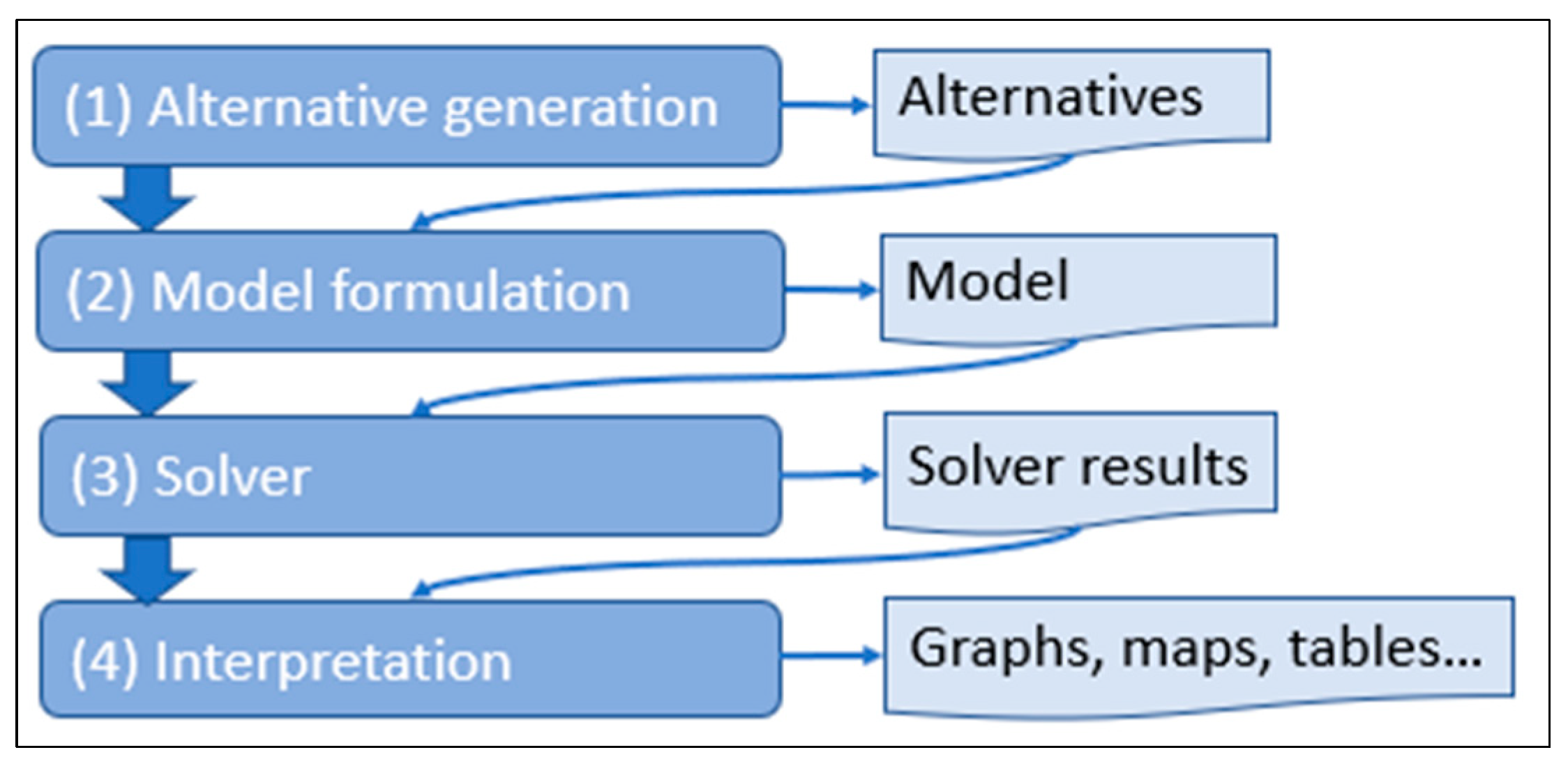
2.1. The Structure of the Management Alternative Generation Process

To model any FEM planning problem, we must identify a set of variables that describe the state of a management unit at any given time, a list of possible management interventions for each management unit, and the “equations of motion” that describe how the state of a management unit changes over time, either with or without management interventions. For the state of a management unit, we assume the following:

• The initial state of a management unit i at time $t_0\le 0$ (e.g., the time when the last intervention occurred in the management unit or the most recent time with available inventory data) can be described by an initial state vector of n attributes $X_{i{t}_0}={[x}_{i{t}_{0}1},x_{i{t}_{0}2}\dots x_{i{t}_{0}n}]$;
• The state of the forest can be described by aggregating the states of individual management units, and the state of one unit does not depend on the state of other units;
• The initial state of each management unit is a known set of values for $X_{i{t}_0}$;
• The set of attributes for a management unit at a given time includes all attributes needed as inputs to the equations of motion and any relevant inputs and outputs associated with that management unit at that time.

We must also be able to update the state vector as a function of any management intervention (or non-intervention) that may occur. This is accomplished through equations of motion, which can be specified as follows:

$$X_{itj}=f\left(X_{i,t-1,j},I_{itj}\right)$$

(1)

where:

t is a time period,

j is a possible state trajectory (“Trajectory” is used here to describe the path followed by the state vector over time, which is governed by the equations of motion and the interventions that are applied to the management unit.) for management unit i,

X_itj is the vector of attributes for management unit i in period t for trajectory j,

I_itj is an intervention that is applied to management unit i in period t on trajectory j.

Note that since the state vector includes both variables that describe the state of the management unit and variables quantifying inputs and outputs, these equations of motion must project (1) growth and yield, (2) management costs, and (3) ecosystem services or attributes for that unit that may enter into objectives or constraints in the optimization stage. However, this does not include attributes that depend on the state of or activities on more than one management unit, such as adjacency restrictions or transportation costs when products can be shipped to more than one destination, depending on what is supplied from other units. Factors such as these must be addressed in the optimization model formulation module (Figure 1—Step 2),

Finally, the set of possible management interventions and the conditions under which they can be applied must be specified. Subsequently, intervention rules are defined by the analyst based on managers’ knowledge of potential interventions and when they can be applied.

iGen provides a flexible environment where users can define each of these elements according to the requirements of their management situation and the available production functions for their problem, so that alternatives can be generated in iGen for virtually any FEM problem. The next section describes how iGen accomplishes this.

2.2. iGen Description

Considering the structure of the FEM problem described in Section 2.1. iGen we apply rule-based system principles to the problem of generating forest management alternatives in the context of an FEMDSS. iGen was written in Python [66]. The user interface was built with open-source Python packages: Taipy [67], Pandas [68], and Plotly [69]. This section describes the iGen elements and how they work together to generate management alternatives for each management unit of a given forest. The iGen elements are designed to enable the application to enumerate all possible ways a given forest management unit could be managed.

2.2.1. iGen Elements

State Variables

iGen requires users to define the set of variables that describe the initial and subsequent states of each management unit based on their specific instance of the FEM problem. The state-descriptor variables must describe all relevant attributes of the management unit and enable the projection of the state of the management unit and any relevant inputs and outputs. In addition to the inputs needed for the equations of motion, users must include state variables for any inputs or outputs that will be relevant in the model-building stage. For a typical FEM problem, state variables could include age, basal area, forest type or species composition, site quality, standing and harvested wood or non-wood product quantities, biomass stock, carbon stock, the carbon sequestration rate, other ecosystem service indicators, equipment requirements, revenues, and the cost of management activities. The state descriptor vector is flexible and can also include a matrix—for example, a tree list and the attributes of each tree in the list.

After defining the state-descriptor variables, the analyst must populate the initial state-descriptor variables based on the initial condition of each management unit in their forest. The initial conditions need not be at time zero. Since data may not be available for the current state of the forest, iGen can update the most recent state data to the present using the equations of motion with no interventions. Thus, for a given instance of iGen, the initial state of each management unit within the forest of interest is specified by a set of initial values for the variables $X_{i{t}_0}={[x}_{i{t}_{0}1},x_{i{t}_{0}2}\dots x_{i{t}_{0}n}]$.

Set of Intervention Types

Interventions are management activities that can alter the character of a forest. The stand of trees in each management unit will grow and develop according to its condition until the managers intervene. Interventions could include any silvicultural treatment, harvesting, or even a business intervention like an ownership change. How management units evolve after an intervention is central to decisions because forest sustainability and growth rates are controlled and either enhanced or harmed by human interventions.

As with the state variables, the interventions in iGen are user-defined. In iGen, an intervention is any event that can be planned, for which the rules for applying the intervention can be defined, and for which the impact of the intervention on the equations of motion can be defined. iGen does not consider random disturbances. Also, non-intervention, where no activity is planned, is treated as a particular type of intervention in iGen and is considered a feasible management option by default, although this can be overridden in the case of mandatory treatment.

In an instance of iGen, the analyst must define the set of valid intervention types, $I=\left[I_1, I_2\dots I_k\right]$, that can occur in their forest. In addition, the initial state of a management unit must include the last intervention that happened in that unit and when it occurred. This is because many rules depend on what kind of intervention occurred last and when it occurred. The initial state is what rule-based system principles call “the set of facts of a beginning state” [44].

Equations of Motion

Left free to grow and affected solely by the forces of nature, forests change, and understanding the change that can occur is critical for forest planning efforts [1]. Equations of motion are used to describe these biological changes mathematically. Understanding and representing those changes is a crucial requirement of the forest planning process. Each state variable must have an equation of motion that describes how that variable evolves over time. The specific equation of motion for a variable $x_n\in X$ is a function of the vector of state variables from the previous period and the intervention type occurring in the period (Equation (2)).

$$x_{i,t,n,j}=f_n\left(X_{i,t-1,j},I_{i,t,j}\right)$$

(2)

where i is the index of the management unit, t is the index of the period, n is the index of the specific state variable, and j is the index of the state trajectory. Note that the intervention $I_{i,t,j}$ can be a non-intervention, in which case the function should compute the development of the management unit in the absence of any management activity. In the case of a regular intervention, the function should calculate the result of the intervention, including any natural growth.

iGen allows the user to specify the equations of motion in several ways. When the equations of motion are very simple, they can be entered directly using a relatively natural interface. For example, the management unit number could be assumed to remain constant over time. This can be specified as follows: MgmUnit = :MgmUnit, where MgmUnit is the state variable for the management unit number. The age of a management unit will, in general, always increase by one period length per period. This can be specified as follows: Age = :Age + PerLen, where Age is the state variable for the age of the stand and PerLen is a global variable for the length of a planning period. Anything that can be expressed as a simple function of one or more of the state variables can similarly be entered using a simple algebraic representation of that function. Where the value of a state variable can be expressed as a simple function of discrete variables, users can specify the equations of motion as a look-up table (e.g., a yield table). For more complex equations of motion, iGen allows the user to call an external user-defined function.

Rule Base

In the context of an AI-RBS, a rule consists of two parts: the IF part and the THEN part. It relates the facts in the IF part to some action in the THEN part. The IF part is called antecedent (or condition), and the THEN part is called consequent (or action). Thus, a simple rule can be expressed as: IF antecedent, THEN consequent. Each rule states that if certain conditions are met, then certain conclusions can be inferred [43,44]. A rule base is a particular type of knowledge base that consists of three essential elements: (i) a set of facts relevant to the beginning state of the system; (ii) a set of rules describing actions that should be taken as a function of the current state; and (iii) a termination criterion that determines when a solution has been found [44]. A rule base aims to encapsulate expert information and provide this knowledge to others through an AI-RBS. In iGen, this knowledge is used to identify and simulate feasible management alternatives for each management unit. These elements are embedded in an information technology system that has at least the following components: (i) a knowledge base with the rules and termination conditions; (ii) a database with the beginning state; and (iii) an inference engine. The inference engine combines reasoning methods and the knowledge base for each state to reach a solution [44,56]. The inference engine goes through the beginning states, checks the applicable rules, and executes the “consequent” for each matched rule whenever the antecedent is found to be true. The inference engine performs these processes until a termination condition is reached. At this point, the inference engine presents a solution to the initial question [70].

In iGen, rules describe the conditions under which interventions may be applied to management units. In other words, a rule is a Boolean function that returns false when an intervention cannot be applied and true when an intervention can be applied. Rules specify the sequence in which interventions can be applied, so they are built on the last intervention that occurred in a management unit and the subsequent evolution of the state of the unit since the last intervention. Thus, given two intervention types, $I_{last}$ and $I_{next}$, we say that a rule $r_n\in R$ is a Boolean function representing the condition for the application of $I_{next}$ given that $I_{last}$ occurred and given the current state of the management unit.

$$R=\left[r_1 {, r}_2\dots r_m\right]$$

(3)

$$r_m=f\left(I_{last} , I_{next} , X_{i,t,j}\right)$$

(4)

where $f$ is a boolean function.

Since the state of a management unit is evolving over time according to the equations of motion, the values of the state variables change over time, so the rules are reevaluated in each period. So, after an occurrence of an $I_{last}$, a rule can return false in a sequence of periods until eventually the rule returns true and the intervention $I_{next}$ can be applied.

As described earlier, a rule has two parts: an antecedent, or condition, and a consequent. Accordingly, once iGen has evaluated the condition for applying a rule, if the rule returns true, the next step is to create a branch where one branch assumes that no intervention will occur and the other assumes that the corresponding active intervention will occur. For each branch, iGen applies the equations of motion for each state variable for the given management unit, in one case with no intervention and in the other with active intervention. If the rule returns false, the next step is to continue assuming that no intervention will occur. Multiple rules may return true for a management unit at a single point in time, so it is possible to create multiple branches, each representing different interventions. For a given node, however, only one no-intervention branch is created.

In summary, an instance of iGen includes a user-defined set of rules $R=\left[r_1 {, r}_2\dots r_m\right]$ according to the specifics of the given forest planning situation. Each instance has a unique set of rules that determine how the interventions can be sequenced to generate a complete set of alternatives. The analyst builds this rule base using natural language expressions consisting of if–then statements based on the current values of the state-descriptor variables.

Network Graph

The management alternatives for each management unit are stored as a network graph. A single, non-loop-directed tree graph [71] is stored for each unit. The first node of each graph contains the initial state data for the corresponding management unit based on the most recent data available for that unit. This may correspond to period zero or any period before period zero of the planning horizon. When the most recent data are from a period prior to period zero, iGen automatically updates the management unit’s state to time zero using the equations of motion. Each node of the graph stores the state of the management unit at a given point in time for a given prescription (i.e., the state trajectory). All the edges of the graph have a length of one period, and the total length of the graph equals the planning horizon plus any nodes representing the state of the management unit prior to period zero.

iGen systematically processes each node in the graph until it reaches an ending point that represents the projected state of the management unit at the end of the planning horizon for that trajectory. For each node that is processed, at a minimum, a new non-intervention node is created for the subsequent period, representing the management unit’s natural development when no active intervention can be applied. When an active intervention can be applied, a new intervention node is also created, and the state variables for the management unit are updated with the equations of motion assuming the intervention occurs. Figure 2 shows an example of a graph developed by iGen and its elements.

The management unit graphs and the underlying database that stores them are the main outputs of the application. The graphs contain all simulated state data (including inputs and outputs) for all possible management alternatives for each management unit according to the rules specified in the rule base. Each node of these graphs has a vector of attributes calculated according to the equations of motion. The resulting graphs show the feasible evolution of the forest state over time for each management prescription.

Relational Database

All the elements of the graphs, including parameters, inputs, outputs, rule bases, and equations of motion, are stored in a relational database.

Table 1. iGen database tables where the elements are stored.

iGen Elements	Input or Output	Tables Where the Elements Are Stored
Set of state variables	Input	Variable
Set of Intervention types	Input	InterventionType
Equations of motion for non-Intervention nodes	Input	Variable
Equations of motion for intervention nodes	Input	RuleCondtion
Rule base	Input	Rule and RuleCondtion
Initial nodes	Input	Nodes
Graph	Output	Nodes
General Parameters	Input	Parameter

shows the key elements and the tables where they are stored. As discussed above, the analyst must specify the set of state variables, the set of intervention types, the equations of motion, the initial state of each management unit, and build the rule base. Those elements are the inputs of the application. Also, the analyst must specify some general parameters such as the planning horizon, period length, name of the model, and other parameters related to the graph shape, as the graph can be visualized as either a table or a graph. Examples of these inputs and outputs are presented in Section 3. Figure 3 shows a diagram of entities and relationships (DER) in an iGen database. The DER also shows how the tables described in Table 1 are related to each other.

The database must be dynamic. Depending on the unique characteristics of the FEM problem, the analyst defines the set of state variables that will describe the management units. Those variables will be rows in the Variable table, and they will be columns in the Nodes table. Also, there must be an equation of motion for each variable. In some cases, the equations of motion used to update the state of a management unit can be stored directly in the Variable table; in other cases, a link is stored to the external function implementing more complex equations of motion.

The analyst can define the MgmUnit attributes according to specific forest characteristics and planning needs. The Nodes table has one attribute to connect each node to its previous node (PreviousNode) and another to connect each node to the last active intervention (LiNode). Also, there is an attribute to identify the node type (NodeType). The other fields in this table are user-defined elements of the set of state variables.

The Rule table is related twice to the InterventionType table, one for the last intervention and one for the next intervention. The Rule condition function compiles all RuleExpression attributes for the same rule when IfOrThen equals “IF”. The equations of motion for each variable and each rule (or a pair I_last–I_next) are stored in the attribute RuleExpression in the RuleCondition table when IfOrThen equals “THEN”.

2.2.2. iGen Algorithm: The Inference Engine

The Inference Engine (I_Engine), as the algorithm of a rule-based system is called, applies the rules to the initial nodes and builds a tree graph, as in Figure 2. To start, I_Engine considers all initial nodes as nodes-to-be-opened and puts them in a list (“nodes-to-open”). The opening process is recursive. New intervention nodes go to the “nodes-to-open” list as they are created, but I_Engine processes an entire non-intervention path until it reaches the end of the planning horizon. When I_Engine finishes the opening process for one node, it sets it as an “opened-node” and then it opens the next node in the “nodes-to-open” list. I_Engine continues this process until the “node-to-open” list is empty.

The node-opening process involves nine steps. Figure 2 provides an example to illustrate the opening process. Figure 4 shows the nine steps in a flow chart.

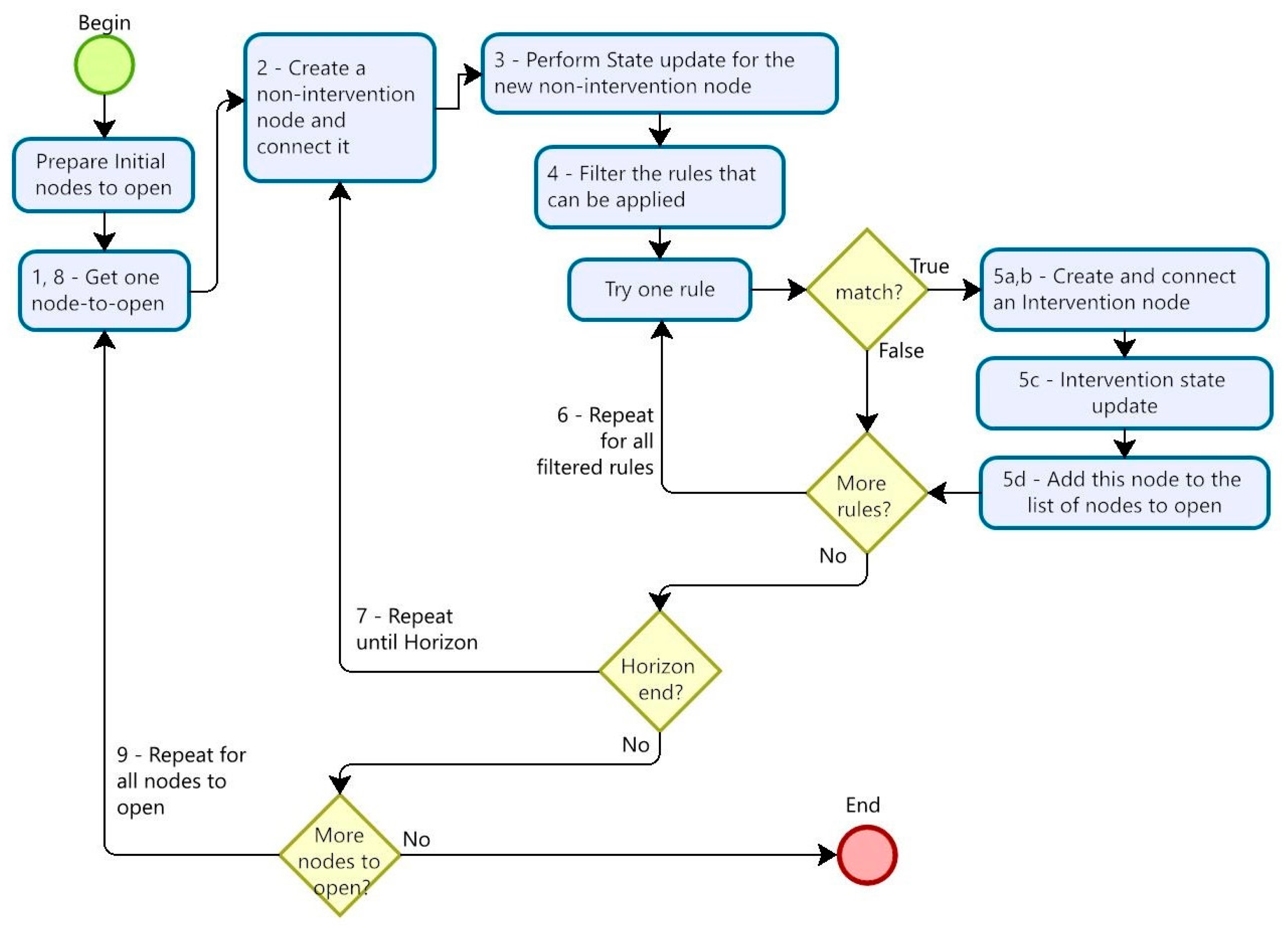
• I_Engine gets an intervention node from the “nodes-to-open” list. In our example (Figure 2), an intervention I₁ happens in node a:I₁.
• I_Engine creates a new non-intervention node in the following period (node #1 in Figure 2) and connects it to the current node being processed (node a:I₁ initially).
• I_Engine uses the equations of motion for each variable to update the forest state for the new node.
• I_Engine filters the rules to select only those with I₁ as the last intervention.
• For the first rule (I_last, I_next) = (I₁, I₂), I_Engine runs the rule Boolean function.
  • If it returns True—i.e., if the conditions for applying the intervention are met—I_Engine:

    (a)

    Creates a node with an intervention I₂ in the same period,

    (b)

    Connects this node to the previous node,

    (c)

    Evaluates the equation of motion for the intervention I2 for each state variable to determine what happens when I₂ occurs, and

    (d)

    Unless the new node occurs at the end of the planning horizon, add this new node to the “node-to-open” list.

  • If it returns False, I_Engine does nothing.
• I_Engine repeats step 5° for each rule in the filtered list of rules.
• I_Engine repeats steps 2° through 6° until the end of the planning horizon.
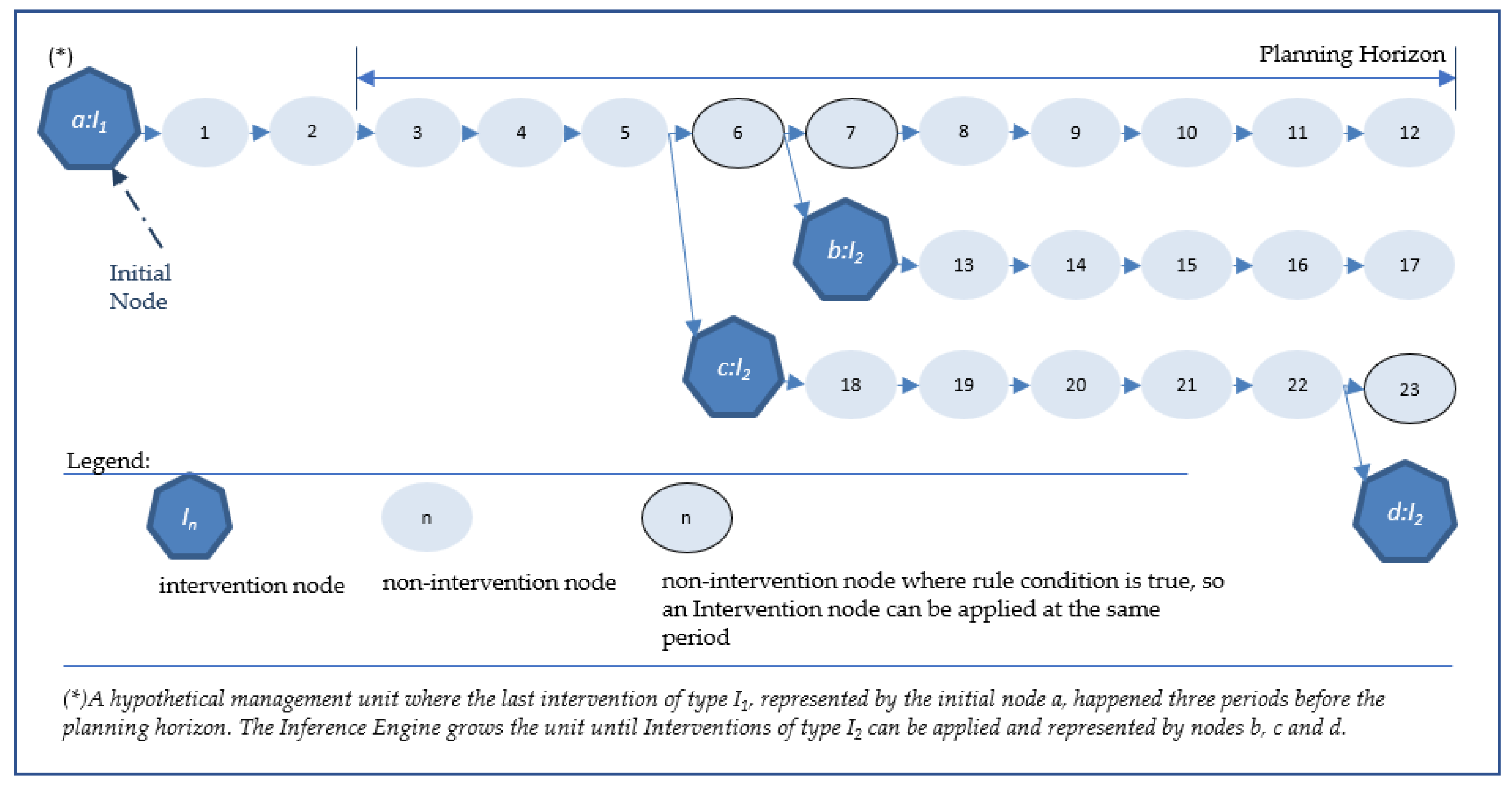
• I_Engine returns to the nodes-to-open list and picks the next one. In our example, node a:I₁ will no longer be in the list, but there will be two others to open: b:I₂ and c:I₂.
• I_Engine repeats steps from 1° to 8° until the node-to-open list is empty.

Applying the above algorithm to the example in Figure 2, I_Engine begins by opening the node a:I₁; it then:

(a)

generates nodes 1 to 12;

(b)

finds a match at node 6, creates node c:I₂, connects it to node 5 (the node previous to node 6), and sets c:I₂ as a “node-to-open”;

(c)

finds a match at node 7, creates node b:I₂, connects it to node 6 (the node previous to node 7), and sets b:I₂ as a “node-to-open”;

(d)

and sets the node a:I₁ as “opened”.

Next, I_Engine opens the node b:I₂ and generates nodes 13 to 17 without creating any new intervention nodes to add to the “nodes to open” list. Next, it opens node c:I₂ and generates nodes from 18 to 23 and the intervention node d:I₂. Node d:I₂ is not added to the “nodes to open” list because it is already at the end of the planning horizon.

The graph in Figure 2 represents four potential prescriptions for this management unit that apply for the span of the planning horizon. Note that these prescriptions share many arcs and nodes within the graph. In fact, all four prescriptions share the same path from the initial node through node 5. Generating prescriptions this way avoids simulating the shared components of each prescription multiple times. These kinds of efficiencies are crucial when there are many management units and many management alternatives for each unit. Additionally, a multicriteria framework typically involves projecting a variety of ecosystem service indicators, production indicators, and social indicators. In these cases, simulating state updates for many management alternatives can consume considerable computer resources. I_Engine can efficiently generate graphs for FEM problems that have thousands of management units with potentially millions of nodes. The iGen framework (the inference engine and the representation of the problem as graphs and rule bases) was developed to optimize the use of planning resources, including computer processing and analysts’ time.

3. Examples

In this section, we apply the concepts of Section 2 to two FEMDSS problems: a natural regeneration problem with shelterwood harvests and a fast-growing plantation/coppice problem. As stated before, the examples are intentionally simple yet very different. By choosing these two specific scenarios, we aimed to highlight the versatility of iGen in addressing diverse forest management challenges and consistently represent the problems despite their differences. The data for the two examples is attached to this article in SQLite^®. The iGen source programs that can run these examples can be found at github.com/SilvanaNobre/iGenPaper.

3.1. Pennsylvania Example

3.1.1. Problem Description

To demonstrate how iGen generates alternatives for a management problem, consider an example of an even-aged forest managed under a natural regeneration regime; we refer to it as the Pennsylvania example. The Pennsylvania example has eight management units, each with an area, age, species composition type (forest type), site quality, and the last intervention that occurred in it. Stand growth is projected with yield curves developed by Gilabert et al. [72] for natural forests in Pennsylvania. Alternatives are generated for a 110-year planning horizon comprised of eleven 10-year periods. For simplicity, we consider only two site qualities and two forest types.

3.1.2. Set of State Variables

The state variables chosen for the Pennsylvania example are typical ones, including area, age, site quality, forest type, yield, yield removed, yield remaining, the last intervention in a unit, and when it occurred. Two additional variables are defined to facilitate the application of the required treatment sequences. The variable named TreatReq specifies a required treatment to apply to the unit, and AfterInt tracks how many periods have elapsed since the last intervention.

3.1.3. Set of Intervention Types

There are two types of interventions in this example: a shelterwood cut (SWC) and an overstory removal (OR). In practice, most, but not all, management units require a SWC prior to an OR to establish advance regeneration. Furthermore, an SWC can only occur after a specified minimum age. On the better site, site 1, an SWC can be done starting at 60 years old. On the poorer site, a SWC can occur only after age 70. An OR should occur in the period following—i.e., 10 years—after an SWC intervention. After an OR, the regeneration process begins, and the age is set to zero. In management units where an inventory cruise has indicated that adequate advance regeneration already exists, an OR can be made without a SWC. A management unit cannot be designated as not requiring a SWC unless it is already old enough to be harvested, and this condition is valid only for the current rotation. Subsequent rotations will assume that an SWC treatment will be required, and the general rule requiring an SWC followed by an OR will apply.

3.1.4. Initial State

With these definitions, we can define the initial state for the management units.

Table 2. Initial State for three management units in the Pennsylvania Example.

Mgm Unit *	Site	Area (acre)	Period	Inter-Vention **	Age (Years)	Species Composition	Treatment Req **	Standing Volume (BF/ac ***)	Removed Volume	Remaining Volume
1	1	100	-6	OR	8	1	SWC	0	0	0
2	1	90	-5	OR	7	2	OR	0	0	0
3	2	120	0	SWC	70	1	OR	6311	2525	3787

(*) Management Unit; (**) SWC-shelterwood cut and OR-overstory removal; (***) Board feet per acre. The initial states of the other management units are provided in the database Pennsylvania, Table Nodes, delivered as Supplementary Material.

shows the initial states of key variables for the first three management units. Note that the columns of the table match the previously defined set of state variables. The age refers to the management unit’s age at the end of the period when the last intervention happened. Management Unit 1 was harvested (OR) 60 years ago and requires a SWC before an OR can be conducted. Management Unit 2 was harvested 50 years ago and does not require a SWC before an OR can be conducted. Management Unit 3 was recently treated with a shelterwood harvest, and an OR intervention must be applied to this unit in the first period.

3.1.5. Equation of Motion

The equations of motion describe the evolution of the state variables over time. An equation of motion must be specified for each variable. In the Pennsylvania example, most variables have simple equations that can be specified directly in iGen. For more complex equations of motion, iGen can call an external function. In this example, only the yield variables require an external function to calculate updated values.

The value of each variable at the previous node is accessed by writing “:variableName”. So, for example, the equation “Site = :Site” specifies that the value of the site quality variable does not change. In this example, this is the case for Site, MgmUnit, Area, SpcComposition, and TreatReq. The expression “Age = :Age + 10” tells iGen to add ten years to the previous node’s Age variable value. While this seems obvious, iGen is meant to be general and flexible in the way specific meanings are assigned to variables. The analyst preparing the problem must give meaning to each variable by writing appropriate equations of motion. For the yield variables, we call the external function PennsylvaniaYield: “=ExtFunctions.PennsylvaniaYield(:Age + 10,[:Site],[:SpcComposition] [9],’stocked’, ’ni’, ‘standing’)”. This function is written by the analyst in Python, and it returns standing, removed, and remaining volume based on the following arguments: age, site, species composition, ecoregion (ecoregion 9 in this case), stocking of the stand, the type of intervention being simulated (e.g., no intervention (‘ni’), SWC vs. OR), and whether the user wants the function to return the total volume (‘standing’), the volume remaining after the intervention, or the volume removed by the intervention. Yields are based on Gilabert et al. [72].

A transcript of this function is provided in Appendix A, and the syntax of the equations of motion can be seen in the databases delivered as Supplementary Material. Database name: Pennsylvania; Table: Variables; Column: NoIntNodeUpdateRule.

3.1.6. Example Rules

As noted earlier, a SWC can happen a minimum of 60 or 70 years after a management unit has been regenerated, depending on the site quality. A rule can therefore be created in iGen to guide the I_Engine during the alternative generation algorithm. The rule for implementing a SWC is shown in

Table 3. The rule for shelterwood cuts in the Pennsylvania example indicates that a shelterwood (SWC) cut can occur after a minimum age after an overstory removal (OR).

Rule Var	Rule Expression
Conditional Part
Age, Site	((:Age >= 60) and (:Site == 1)) or ((:Age >= 70) and (:Site == 2))
TreatReq	(:TreatReq == ‘SWC’)
Consequent Part
MgmUnit	= :MgmUnit
Site	= :Site
Area	= :Area
AfterInt	= 0
Age	= 5
SpcComposition	= :SpcComposition
TreatReq	= ‘SWC’
Yield	= ExtFunctions.PennsylvaniaYield (:Age,[:Site], [:SpcComposition], [9],’stocked’,’SWC’, ‘Standing’)
YRemoved	= ExtFunctions.PennsylvaniaYield (:Age,[:Site], [:SpcComposition], [9],’stocked’,’SWC’, ‘Removed’)
yRemaining	= ExtFunctions.PennsylvaniaYield (:Age,[:Site], [:SpcComposition], [9],’stocked’,’SWC’, ‘Remaining’)

.

The conditional part of a rule specifies when a particular intervention can be applied. The consequent part of the rule in Table 3 describes how the management unit’s state will be updated after an SWC occurs. It is important to note that rules are evaluated based on the state of the unit at the point in time when the intervention would be applied. To accomplish this, before a rule is evaluated, the state of the management unit is always updated first as if no intervention had occurred. Then, the rule is applied based on the new, updated state. The conditional part is evaluated based on this updated state, and if the conditional part returns “true” then the intervention state updates are made based on the state of the unit just prior to the intervention—that is, based on the state at the new non-intervention node.

The next rule establishes the conditions under which an OR can occur following an SWC. Since the OR should occur immediately after a SWC intervention, the RuleCondition states that when the last intervention was an SWC and AfterInt == 1, then an OR must occur. And when the I_Engine gets a match for this rule, the consequent part is the same as the rule described in Table 3, with the following exceptions: (i) age is set to five (we assume that the intervention happened at the midpoint of the period) on average by the end of the period (Age = 5), and (ii) the treatment required will turn to SWC (TreatReq = ‘SWC’); (iii) and the yield functions are called with the parameter ‘OR’ for the intervention type parameter.

Table 4. The rule for when an overstory removal can occur without a shelterwood harvest in the Pennsylvania example.

Rule Var	Rule Expression
Conditional Part
TreatReq	(:TreatReq == ‘OR’)
Consequent Part
MgmUnit	= :MgmUnit
Site	= :Site
Area	= :Area
AfterInt	= 0
Age	= 5
SpcComposition	= :SpcComposition
TreatReq	= ‘SWC’
Yield	= ExtFunctions.PennsylvaniaYield (:Age,[:Site],[:SpcComposition], [9],’stocked’,’OR1′, ‘Standing’)
YRemoved	= ExtFunctions.PennsylvaniaYield(:Age,[:Site],[:SpcComposition], [9],’stocked’,’OR1′, ‘Removed’)
yRemaining	= ExtFunctions.PennsylvaniaYield(:Age,[:Site],[:SpcComposition], [9],’stocked’,’OR1′, ‘Remaining’)

shows the rule for management units that do not require an SWC prior to conducting an OR, i.e., management units with LastIntervention = ‘OR’ and TreatReq = ‘OR’. Note that in the consequent part of this rule, TreatReq is set to ‘SWC’ so that in the next rotation, a SWC will be required. Also, the yield functions are called with the parameter ‘OR1.’ This is because the yield for an OR will be greater when no SWC has been conducted prior to the OR.

3.1.7. Result

The I_Engine applies the rules to the initial state and generates one network graph containing all possible alternatives for each management unit. Data related to all graphs is stored in the database table Nodes, and the results can be visualized as either a graph or a table. As an example, Figure 5 presents the graph for management unit 2. This management unit is one where an inventory cruise indicated that an OR can be conducted without a SWC. Figure 5 shows that the last intervention in unit 2 was an OR that occurred 50 years ago. From period −5, the I_Engine grows the forest until period 0 (zero), at which point unit 2 reaches age 57. Then, according to the rules, the I_Engine opens a non-intervention node (which will leave the unit to grow one period more) and an OR node. Following the non-intervention path, the I_Engine generates the default non-intervention node and one OR node for each period until the end of the planning horizon. The program then begins opening the intervention nodes that have not been processed. After each OR node, the program grows the forest until age 65, because this unit is site 1 (Table 2), and then begins creating SWC-OR alternatives for each period until the end of the planning horizon.

Table 5. Data from the Nodes Table for the Pennsylvania Example corresponding to selected nodes from Figure 5.

NodeId	Previous Node	LiNode	Period	Intervention	Age	After-Int	Yield	Yield Removed	Yield Remaining
43	41	2	1	OR	5	0	13,432	13,432
197	43	43	2	ni	15	1	217
198	197	43	3	ni	25	2	1821
199	198	43	4	ni	35	3	4528
200	199	43	5	ni	45	4	7510
201	200	43	6	ni	55	5	10,362
203	201	43	7	SWC	65	0	12,949	5180	7770

NodeId: Node identification number; PreviousNode: the NodeID for the previous node on the graph; LiNode: NodeID for the most recent Intervention Node; OR represents an overstory removal; “ni” indicates no intervention; SWC represents a shelterwood cut; After-Int gives the number of periods since the previous intervention; yields are in board feed per acre.

shows the rows of the Nodes table corresponding to the nodes highlighted in Figure 5. Node 43, an OR node, is the first one of the set, and the following nodes refer to it in the column LiNode (Last Intervention Node).

Management units 1 and 3 require an SWC before an OR treatment can be applied. This is indicated by setting the field TreatReq = “SWC”. I_Engine applies a different set of rules for these units and generates similar graphs, but with different sequences. The graphs for units 1 and 3 are in HTML files included with the Supplementary Material. Filenames: Pennsylvana1.html and Pennsylvania2.html.

3.2. Plantation-Coppice Example

3.2.1. Problem Description

The second example of a FEM problem is a fast-growing plantation under a short-rotation coppice regime that produces biomass or pulpwood [73,74]. We call it the Plantation–Coppice example. This example has seven management units, with each belonging to a stratum and having attributes such as area, age, rotation count, and the last intervention that occurred in it. Unlike the first example, the Plantation–Coppice example has a yield table with two entries: stratum and age. Alternatives are generated for a 21-year horizon comprised of twenty-one 1-year periods. For simplicity, we consider only two strata.

3.2.2. State Variables

As with the first example, the state variables for the Plantation–Coppice example management units are the typical ones, such as area, age, stratum, rotation count, yield, the last intervention in a unit, and when it occurred. The rotation count is 1 after the initial planting, 2 after the first coppice, and so on. When a clearcut is followed by a renewal planting, the rotation count is reset to 1.

3.2.3. Potential Interventions

The two types of interventions are based on a regular coppice regime: a clear cut followed by a renewal planting (CCR) or a clear cut followed by sprouting from stumps (CCS). In this example, only one CCS is allowed, so after a coppice harvest, the next clear cut must be followed by a renewal (CCR) to plant new genetic material [75].

3.2.4. Initial State

With these definitions, we can define the initial state for each management unit.

Table 6. Plantation/Coppice example initial state for four management units.

Mgm Unit	Stratum	Area	Period	Last Intervention	Age	Rotation Count	Yield
1	1	40	−2	CCR	0	1	0
2	1	50	−4	CCR	0	1	0
3	2	54	−2	CCR	0	1	0
4	1	20	−1	CCS	0	2	0

shows the data for the first four. The columns of the table match the set of state variables. The age and the yield refer to the management unit’s age in the period when the last intervention happened. All ages are zero when a clear cut occurs; some are in the first rotation after the renewal, and others are in the second rotation following a CCS intervention.

3.2.5. Equation of Motion

As in the Pennsylvania example, in the Plantation–Coppice example most variables have simple equations of motion with no intervention. The equations of motion for MgmUnit, Area, Stratum, and RotationCount specify that the value of the state variable does not change. For example, they are written like “Stratum = :Stratum”. In this example, the equation for age is “Age = :Age + 1”. Only the yield variable requires a function (SearchTable) to select yield coefficients from a production table. For this kind of equation of motion, I_Engine can read a user table (Productivity) using the specified entries (Stratum, Age) to return the appropriate value (Volume). And it is written like this: “Yield = SearchTable(‘Productivity’, (:Stratum, :Age + 1), ’Volume’)” (The syntax of the equations of motion for this example can be seen in the databases delivered as Supplementary Material. Database name: Coppice; Table: Variables; Column: NoIntNodeUpdateRule).

3.2.6. Example Rules

There are three rules related to the two intervention types in the Coppice Example. After a CCR, we can have either another CCR or a CCS. However, a CCR must follow a CCS. The rule conditions for the three possibilities are the same. The management units can only be cut at ages 6 or 7 if they have reached a minimum yield of 200 m³/ha. However, in periods 1 to 3, older ages up to 9 years can also be cut. The condition part of these rules is written by the analyst within the iGen context as “((6 <= :Age <= 7) or (1 <= :Period <=3 and 6 <= :Age <= 9)) and (:Yield >= 200)”

When any of these rules is satisfied, a new intervention node is generated, and I_Engine applies the consequent part of the rules (intervention state updates). The equations of motion for Area, MgmUnit, and Stratum specify that they remain the same; RotationCount is set to a value of 1 when a CCR occurs and a value of 2 when a CCS occurs, according to the logic of a coppice regime; and Age and Yield are set to zero.

3.2.7. Results

As in the Pennsylvania example, the I_Engine generates a graph for each management unit. Figure 6 presents the graph for management unit 1 of the Plantation–Coppice example. Unit 1 was clearcut and renewed two years before the beginning of the horizon; therefore, by the fourth period, it will be possible to cut this unit again. This results in three alternatives in the fourth period: conducting a CCR, a CCS, or doing nothing and letting the forest grow (no intervention). This pattern repeats in the following years, according to the rules. For unit 3, located in a less productive stratum, it is impossible to have a clear cut at age six because the minimum yield will not be reached yet, making fewer alternatives for that unit, as shown in file Coppice3.html delivered as complementary material.

Again, I_Engine applies the equation of motion to previous states and saves each state in the Nodes table.

Table 7. Data from the Nodes Table for the Plantation/Coppice Example corresponding to selected nodes from Figure 6.

Node Id	Previous Node	LiNode	Period	Age	Rotation Count	Yield
214	15	15	5	1	2	60
215	214	15	6	2	2	100
216	215	15	7	3	2	140
217	216	15	8	4	2	190
218	217	15	9	5	2	210
219	218	15	10	6	2	230

Node Id: Identification number of the node; Previous Node: the node that is immediately before the node; LiNode: last intervention node that comes before the node.

shows the part of this table corresponding to the selected nodes in Figure 6. The CCS node in period 4 is node #15. Nodes 218 to 219 have node 15 as the last intervention (LiNode). Note that the initial value of RotationCount for unit 1 was 1 (Table 6), but the CCS intervention changes this value to 2.

4. Discussion and Conclusions

The objective of this work was to develop a system for generating alternatives for a FEMDSS that can be applied to virtually any FEM problem. We call this system iGen. iGen uses an AI-RBS approach to provide a flexible, efficient, standardized, and comprehensive environment for generating management alternatives. iGen’s flexibility can also be attributed to three key features. First, users can define the state variable vector for management units according to the available data, models (production functions), and objectives of their problem instance. In fact, users must define the state variables because iGen assumes almost nothing about this. Second, users can and must also define the types of interventions that can be applied to each type of management unit and create a rule base describing the conditions under which each intervention can be applied. Finally, users specify the equations of motion that determine how the state vector for each management unit will be updated over time, depending on which, if any, interventions are applied. This is perhaps the most challenging part of creating a truly instance-agnostic FEM alternative generator. However, we have reviewed the most common types of equations of motion and have provided a variety of ways to specify them, from simple algebraic expressions of the state variables to input matrices (look-up tables) to calling user-provided external functions. This last feature, in particular, should provide users with considerable flexibility in implementing their particular equations of motion.

With versatile tools such as iGen, researchers and practitioners can enhance the creation of a comprehensive LP solution space (feasible region). Consequently, during subsequent phases 2 and 3 (Figure 1), the solver has an increased potential to identify the absolute optimal solution. The more accurate we are in building the feasible region, the closer we get to the optimal solution.

Other than this basic structure, virtually everything in an iGen problem instance is user-defined. Thus, while iGen provides a structure for building an FEM planning instance, it is essentially a “blank slate” where developers define the state variables for management units, the rules for their management, and the production functions that describe how management units develop and the associated inputs and outputs under each management alternative. iGen uses these key elements to simulate all possible management prescriptions for each management unit and stores the resulting information in a database that uses a flexible and efficient network structure, reinforcing some authors’ assertions about the efficiency of network representation [76] versus, for example, a matrix representation. The database must be flexible to accommodate the fact that most of the information that it must store is based on user-defined elements. It is efficient because its network structure—as opposed to the matrix structure typically employed in this step (hence the term “matrix generator”) —eliminates redundancy and facilitates easy retrieval of information for the generation of the optimization models that will ultimately be used to determine the Pareto frontier for a given FEM problem. Of course, only time will tell if there are problem instances that cannot be modeled by the current version of iGen. We are optimistic, however, that any such limitations can be addressed in future versions of the software without fundamentally changing its structure.

While each problem is unique in terms of the specific details of these elements, all FEM alternative generation problems involve the same key elements: the state description, the possible interventions, the rules for applying interventions, and the equations of motion for updating the state variables under each management regime. The fundamental contribution of the iGen methodology is the identification of these fundamental elements of the FEM alternative generation process, their definition in a very general way, and the creation of a modeling framework that gives forest planners the flexibility to specify each of these elements in a way that is required by their particular FEM problem. To our knowledge, this has not been done in literature. Ultimately, we hope that iGen—or at least the underlying concepts—will be used by practitioners and other researchers, providing the forest planning community with a common framework for building FEMDSSs.

Besides its generality, a key feature of the iGen approach to alternative generation is its efficiency. First, it efficiently simulates each possible alternative for each management unit. iGen’s recursive algorithm for generating a graph of alternatives for each management unit ensures that each arc of the graph needs to be simulated only once. Each node in the graph is unique, so there is no duplication of information storage, and all data related to the management alternatives needed for building the LP model or MIP model is contained in the database. In addition, the rules specified by the user guarantee that only acceptable and feasible alternatives will be created.

Furthermore, because the graph provides a natural, visual representation of the alternatives, it is easy for users to interpret and verify the data generated for each alternative. Since the equations of motion and intervention rules are written by the forest planning analyst and not by the programmer, the analyst has full control of the model. This visual interface allows the analyst to verify and validate the alternatives generated and better understand the relationships between the evolution of the forest state and the management prescriptions before building any optimization models. The analyst can also check the validity of the coefficients that will be used to build an LP or MIP model before it is built to ensure that the model’s simulations are producing valid results. This is much easier than reviewing the coefficients of, for example, an LP model.

Another key feature of the FEMDSS that iGen is a part of is that the alternative generation process is separate from the model-building process. While other FEMDSSs also do this [17,39], it is worth highlighting here. In many cases, the alternative generation process only needs to be done once, while the optimization model-building process will often need to be performed multiple times. A single set of management alternatives can be used to build multiple optimization models—for example, when finding the Pareto frontier of a multiobjective planning problem. A well-defined, flexible structure that provides an interface between the generation of management alternatives and the model formulation phase improves the transparency and clarity of the processes for the forest analyst.

While not addressed in this paper, the network structure of the management alternative database produced by iGen provides a natural structure for constructing an LP or MIP model. Exactly how this is done will be the topic of a forthcoming paper, but it is easy to extract the information needed to build objective functions and constraints for LP and MIP models from the database. Specifically, one can easily construct area (for LP) or logical (for MIP) constraints, as well as accounting constraints, for any ecosystem service that was included in the state variable definition. Furthermore, this is easily done for a variety of model structures, including Model I, Model II [77], and others. Certain kinds of constraints, such as flow [25], supply chain and market [78], transportation and logistics [79], adjacency [80], labor [81], and equipment constraints [82], can also be built, but will require other inputs that are not needed in the alternative generation stage and that can be input at the LP or MIP model-building stage.

iGen is currently written to only simulate deterministic processes. It is not written to accommodate stochastic equations of motion. In principle, it would not be too hard to modify iGen to allow this, but in practice, this could result in extremely large output databases for realistically sized FEM problems. Nevertheless, this may be an interesting problem for future development of the system.

The code for iGen is open source, and datasets and equations of motion sample code for different types of forests are provided on github.com/SilvanaNobre/iGenPaper. We hope this system will be a valuable resource for practitioners and researchers interested in the development of FEMDSSs.

References

1. Bettinger, P.; Boston, K.; Siry, J.P.; Grebner, D.L. Forest Management and Planning, 2nd ed.; Elsevier Inc.: Amsterdam, The Netherlands, 2017; ISBN 9780128094761. [Google Scholar]
2. Buongiorno, J.G.J. Decision Methods for Forest Resource Management, 1st ed.; Elsevier Academic Press: Cambridge, MA, USA, 2003; ISBN 978-0121413606. [Google Scholar]
3. Borges, J.G.; Nordström, E.M.; Garcia-Gonzalo, J.; Hujala, T.; Trasobares, A. Computer-Based Tools for Supporting Forest Management. The Experience and the Expertise World-Wide, 1st ed.; Department of Forest Resource Management, Swedish University of Agricultural Sciences: Umea, Sweden, 2014. [Google Scholar]
4. Rönnqvist, M.; D’Amours, S.; Weintraub, A.; Jofre, A.; Gunn, E.; Haight, R.G.; Martell, D.; Murray, A.T.; Romero, C. Operations Research Challenges in Forestry: 33 Open Problems. Ann. Oper. Res. 2015, 232, 11–40. [Google Scholar] [CrossRef]
5. Radke, N.; Yousefpour, R.; von Detten, R.; Reifenberg, S.; Hanewinkel, M. Adopting Robust Decision-Making to Forest Management under Climate Change. Ann. For. Sci. 2017, 74, 43. [Google Scholar] [CrossRef]
6. Franca, L.C.D.; Acerbi, F.W.; Silva, C.; Monti, C.A.U.; Ferreira, T.C.; Santana, C.J.D.; Gomide, L.R. Forest Landscape Planning and Management: A State-of-the-Art Review. Trees For. People 2022, 8, 100275. [Google Scholar] [CrossRef]
7. Bettinger, P.; Chung, W. The Key Literature of, and Trends in, Forest-Level Management Planning in North America, 1950–2001. Int. For. Rev. 2004, 6, 40–50. [Google Scholar] [CrossRef]
8. Hujala, T.; Khadka, C.; Wolfslehner, B.; Vacik, H. Review. Supporting Problem Structuring with Computer-Based Tools in Participatory Forest Planning. For. Syst. 2013, 22, 270–281. [Google Scholar] [CrossRef]
9. Pasalodos-Tato, M.; Makinen, A.; Garcia-Gonzalo, J.; Borges, J.G.; Lamas, T.; Eriksson, L.O. Review. Assessing Uncertainty and Risk in Forest Planning and Decision Support Systems: Review of Classical Methods and Introduction of Innovative Approaches. For. Syst. 2013, 22, 282–303. [Google Scholar] [CrossRef]
10. Pascual, A.; Giardina, C.P.; Povak, N.A.; Hessburg, P.F.; Asner, G.P. Integrating Ecosystem Services Modeling and Efficiencies in Decision-Support Models Conceptualization for Watershed Management. Ecol. Model. 2022, 466, 109879. [Google Scholar] [CrossRef]
11. Borges, J.G.; Falcao, A.O.; Miragaia, C.; Marques, P.; Marques, M. A Decision Support System for Forest Ecosystem Management in Portugal. In Proceedings of the Systems Analysis in Forest Resources, Snowmass Village, CO, USA, 27–30 September 2000; Arthaudf, G.J., Barrett, T.M., Eds.; Springer: Dordrecht, The Netherlands, 2003; Volume 7, pp. 155–163. [Google Scholar]
12. Næsset, E. A Spatial Decision Support System for Long-term Forest Management Planning by Means of Linear Programming and a Geographical Information System. Scand. J. For. Res. 1997, 12, 77–88. [Google Scholar] [CrossRef]
13. Siitonen, M.; Anola-Pukkila, A.; Haara, A.; Harkonen, K.; Redsven, V.; Salminen, O.; Suokas, A. Mela Handbook, 2nd ed.; The Finish Forest Research Institute: Helsinki, Finland, 2001; Volume 1. [Google Scholar]
14. Wikström, P.; Edenius, L.; Elfving, B.; Eriksson, L.O.; Lämås, T.; Sonesson, J.; Öhman, K.; Wallerman, J.; Waller, C.; Klintebäck, F. The Heureka Forestry Decision Support System: An Overview. Math. Comput. For. Nat. Resour. Sci. 2011, 3, 87–95. [Google Scholar]
15. Rodriguez, L.C.E.; Stansfield, W.F. ForXGen—A Matrix Generator for Use with ForxCel; School of Forestry: Flagstaff, AZ, USA, 1995. [Google Scholar]
16. Laacke, R.J. Building a Decision-Support System for Ecosystem Management—Klems. AI Appl. 1995, 9, 115–127. [Google Scholar]
17. Packalen, T.; Marques, A.F.; Rasinmäki, J.; Rosset, C.; Mounir, F.; Rodriguez, L.C.E.; Nobre, S.R. Review. A Brief Overview of Forest Management Decision Support Systems (FMDSS) Listed in the FORSYS Wiki. For. Syst. 2013, 22, 263–269. [Google Scholar] [CrossRef]
18. Kaya, A.; Bettinger, P.; Boston, K.; Akbulut, R.; Ucar, Z.; Siry, J.; Merry, K.; Cieszewski, C. Optimisation in Forest Management. Curr. For. Rep. 2016, 2, 1–17. [Google Scholar] [CrossRef]
19. Constantino, M.; Martins, I.; Borges, J.G. A New Mixed-Integer Programming Model for Harvest Scheduling Subject to Maximum Area Restrictions. Oper. Res. 2008, 56, 542–551. [Google Scholar] [CrossRef]
20. Goycoolea, M.; Murray, A.T.; Barahona, F.; Epstein, R.; Weintraub, A. Harvest Scheduling Subject to Maximum Area Restrictions: Exploring Exact Approaches. Oper. Res. 2005, 53, 490–500. [Google Scholar] [CrossRef]
21. Goycoolea, M.; Murray, A.; Vielma, J.P.; Weintraub, A. Evaluating Approaches for Solving the Area Restriction Model in Harvest Scheduling. For. Sci. 2009, 55, 149–165. [Google Scholar]
22. Könny, N.; Tóth, S.F. A Cutting Plane Method for Solving Harvest Scheduling Models with Area Restrictions. Eur. J. Oper. Res. 2013, 228, 236–248. [Google Scholar] [CrossRef]
23. Vielma, J.P.; Murray, A.T.; Ryan, D.M.; Weintraub, A. Improving Computational Capabilities for Addressing Volume Constraints in Forest Harvest Scheduling Problems. Eur. J. Oper. Res. 2007, 176, 1246–1264. [Google Scholar] [CrossRef]
24. Hernandez, M.; Gómez, T.; Molina, J.; León, M.A.; Caballero, R. Efficiency in Forest Management: A Multiobjective Harvest Scheduling Model. J. For. Econ. 2014, 20, 236–251. [Google Scholar] [CrossRef]
25. Hof, J.G.; Pickens, J.B.; Barlett, E.T. A Maxmin Approach to Nondeclining Yield Timber Harvest Scheduling Problems. For. Sci. 1986, 32, 653–666. [Google Scholar]
26. Martins, I.; Alvelos, F.; Cerveira, A.; Kaspar, J.; Marusak, R. Solving a Harvest Scheduling Optimization Problem with Constraints on Clearcut Area and Clearcut Proximity. Int. Trans. Oper. Res. 2023, 30, 3930–3948. [Google Scholar] [CrossRef]
27. Xavier, A.M.D.; Freitas, M.D.C.; Fragoso, R.M.D. Management of Mediterranean Forests—A Compromise Programming Approach Considering Different Stakeholders and Different Objectives. For. Policy Econ. 2015, 57, 38–46. [Google Scholar] [CrossRef]
28. Marques, S.; Bushenkov, V.A.; Lotov, A.v.; Marto, M.; Borges, J.G. Bi-Level Participatory Forest Management Planning Supported by Pareto Frontier Visualization. For. Sci. 2020, 66, 490–500. [Google Scholar] [CrossRef]
29. Marques, M.; Reynolds, K.M.; Marques, S.; Marto, M.; Paplanus, S.; Borges, J.G. A Participatory and Spatial Multicriteria Decision Approach to Prioritize the Allocation of Ecosystem Services to Management Units. Land 2021, 10, 747. [Google Scholar] [CrossRef]
30. Marto, M.; Marques, M.; Borges, J.G.; Tomé, M. Forestry Databases to Simulators and Decision Support Systems; Technical Report No. 01/2015 (Version 2.6); Center for Forestry Studies: Lisbon, Portugal, 2015. [Google Scholar]
31. Potter, M.W.; Kessell, S.R.; Cattelino, P.J. FORPLAN: A FORest Planning LANguage and Simulator. Environ. Manag. 1979, 3, 59–72. [Google Scholar] [CrossRef]
32. Eriksson, L.O. Planning under Uncertainty at the Forest Level: A Systems Approach. Scand. J. For. Res. 2006, 21, 111–117. [Google Scholar] [CrossRef]
33. Nobre, S.R.; Eriksson, L.O.; Trubins, R. The Use of Decision Support Systems in Forest Management: Analysis of FORSYS Country Reports. Forests 2016, 7, 72. [Google Scholar] [CrossRef]
34. Skovsgaard, J.P.; Vanclay, J.K. Forest Site Productivity: A Review of the Evolution of Dendrometric Concepts for Even-Aged Stands. Forestry 2008, 81, 13–31. [Google Scholar] [CrossRef]
35. Shifley, S.R.; He, H.S.; Lischke, H.; Wang, W.J.; Jin, W.; Gustafson, E.J.; Thompson, J.R.; Thompson, F.R.; Dijak, W.D.; Yang, J. The Past and Future of Modeling Forest Dynamics: From Growth and Yield Curves to Forest Landscape Models. Landsc. Ecol. 2017, 32, 1307–1325. [Google Scholar] [CrossRef]
36. Miles, P.D. Forest Inventory and Analysis Data for FVS Modelers. In Proceedings of the Third Forest Vegetation Simulator Conference, Fort Collins, CO, USA, 13–15 February 2007; Havis, R.N., Crookston, N.L., Eds.; Rocky Mountain Research Station: Fort Collins, CO, USA, 2008; Volume 54, pp. 125–129. [Google Scholar]
37. de Oliveira, E.B.; de Oliveira, Y.M.M.; Hafley, W.L. Software to predict Growth and Yield for p.ellioti and p.taeda in southern Brazil. Pesqui. Agropecu. Bras. 1991, 26, 149–151. [Google Scholar]
38. Gupta, R.; Sharma, L.K. The Process-Based Forest Growth Model 3-PG for Use in Forest Management: A Review. Ecol. Model. 2019, 397, 55–73. [Google Scholar] [CrossRef]
39. Eriksson, L.O.; Bergh, J. A Tool for Long-Term Forest Stand Projections of Swedish Forests. Forests 2022, 13, 816. [Google Scholar] [CrossRef]
40. Mcdermott, J. RI: A Rule-Based Configurer of Computer Systems. Artif. Intell. 1982, 19, 39–88. [Google Scholar] [CrossRef]
41. Waterman, D.A.; Hayes-Roth, F. Pattern-Directed Inference Systems, 1st ed.; Waterman, D.A., Ed.; Academic Press: New York, NY, USA, 1978; ISBN 978-0-12-737550-2. [Google Scholar]
42. Amarel, S.; Brown, J.S.; Buchanan, B.; Hart, P.; Kulikowski, C.; Martin, W.; Pople, H. Reports of Panel on Applications of Artificial Intelligence. In Proceedings of the Fifth International Joint Conference on Artificial Intelligence, Cambridge, MA, USA, 22–25 August 1977; pp. 994–1006. [Google Scholar]
43. Duda, R.; Hart, P.E.; Nilsson, N.J.; Sutherland, G.L. Network Representations in Rule-Based Inference Systems 1. In Pattern Directed Inference Systems; Waterman, D.F., Ed.; Academic Press: New York, NY, USA, 1978; ISBN 0127375503. [Google Scholar]
44. Grosan, C.; Abraham, A. Rule-Based Expert Systems. In Intelligent Systems; Grosan, C., Abraham, A., Eds.; Springer: Berlin/Heidelberg, Germany, 2011; pp. 149–185. ISBN 978-3-642-21004-4. [Google Scholar]
45. Minutolo, A.; Esposito, M.; De Pietro, G. Optimization of Rule-Based Systems in MHealth Applications. Eng. Appl. Artif. Intell. 2017, 59, 103–121. [Google Scholar] [CrossRef]
46. Gustafson, E.J.; Crow, T.R. Forest Management Alternatives in the Hoosier National Forest. J. For. 1994, 92, 28–29. [Google Scholar] [CrossRef]
47. McDill, M.E. RxWrite: An Information Management Tool for Minnesota’s Generic Environmental Impact Statement on Timber Harvesting. In Proceedings of the E4-Management Science and Operations Research Session at SAF National Convention, Indianapolis, IN, USA, 7 November 1993. [Google Scholar]
48. Williams, S.B.; Roschke, D.J.; Holtfrerich, D.R. Designing Configurable Decision-Support Software—Lessons Learned. AI Appl. 1995, 9, 103–114. [Google Scholar]
49. Albert, M. Predicting the selection of elite trees in mixed-species stands—A rule-based algorithm for silvicultural decision support systems. Allg. Forst Jagdztg. 2002, 173, 153–161. [Google Scholar]
50. Stansfield, S.A. ANGY: A Rule-Based Expert System for Automatic Segmentation of Coronary Vessels from Digital Subtracted Angiograms. IEEE Trans. Pattern Anal. Mach. Intell. 1986, PAMI-8, 188–199. [Google Scholar] [CrossRef]
51. Michael, D.J.; Nelson, A.C. HANDX: A Model-Based System for Automatic Segmentation of Bones from Digital Hand Radiographs. IEEE Trans. Med. Imaging 1989, 8, 64–69. [Google Scholar] [CrossRef] [PubMed]
52. Phan, P.; Ouellet, J.; Mezghani, N.; de Guise, J.A.; Labelle, H. A Rule-Based Algorithm Can Output Valid Surgical Strategies in the Treatment of AIS. Eur. Spine J. 2015, 24, 1370–1381. [Google Scholar] [CrossRef]
53. Savadjiev, P.; Chong, J.; Dohan, A.; Vakalopoulou, M.; Reinhold, C.; Paragios, N.; Gallix, B. Demystification of AI-Driven Medical Image Interpretation: Past, Present and Future. Eur. Radiol. 2019, 29, 1616–1624. [Google Scholar] [CrossRef]
54. Al Fryan, L.H.; Shomo, M.I.; Alazzam, M.B.; Rahman, M.A. Processing Decision Tree Data Using Internet of Things (IoT) and Artificial Intelligence Technologies with Special Reference to Medical Application. BioMed Res. Int. 2022, 2022, 8626234. [Google Scholar] [CrossRef] [PubMed]
55. Hooda, R.; Joshi, V.; Shah, M. A Comprehensive Review of Approaches to Detect Fatigue Using Machine Learning Techniques. Chronic. Dis. Transl. Med. 2022, 8, 26–35. [Google Scholar] [CrossRef] [PubMed]
56. Matsuyama, T. Expert Systems for Image Processing: Knowledge-Based Composition of Image Analysis Processes. Comput. Vis. Graph. Image Process. 1989, 48, 22–49. [Google Scholar] [CrossRef]
57. Abdullah, U.; Shaheen, M.; Ujager, F.S. Implementing Rule-Based Healthcare Edits. Ksii Trans. Internet Inf. Syst. 2022, 16, 116–132. [Google Scholar] [CrossRef]
58. Beccali, M.; Bonomolo, M.; Martorana, F.; Catrini, P.; Buscemi, A. Electrical Hybrid Heat Pumps Assisted by Natural Gas Boilers: A Review. Appl. Energy 2022, 322, 119466. [Google Scholar] [CrossRef]
59. Pean, T.Q.; Salom, J.; Costa-Castello, R. Review of Control Strategies for Improving the Energy Flexibility Provided by Heat Pump Systems in Buildings. J. Process Control 2019, 74, 35–49. [Google Scholar] [CrossRef]
60. Igder, M.A.; Liang, X.D.; Mitolo, M. Service Restoration Through Microgrid Formation in Distribution Networks: A Review. IEEE Access 2022, 10, 46618–46632. [Google Scholar] [CrossRef]
61. Pizarro, P.N.; Hitschfeld, N.; Sipiran, I.; Saavedra, J.M. Automatic Floor Plan Analysis and Recognition. Autom. Constr. 2022, 140, 104348. [Google Scholar] [CrossRef]
62. Wu, C.S.; Liu, Y.C. Rule-Based Control of Weld Bead Width in Pulsed Gas Tungsten Are Welding (GTAW). Proc. Inst. Mech. Eng. Part B-J. Eng. Manuf. 1996, 210, 93–98. [Google Scholar] [CrossRef]
63. Fu, Y.Y.; Neill, Z.O.; Wen, J.; Pertzborn, A.T.; Bushby, S. Utilizing Commercial Heating, Ventilating, and Air Conditioning Systems to Provide Grid Services: A Review. Appl. Energy 2022, 307, 118133. [Google Scholar] [CrossRef]
64. Yousefli, A.; Heydari, M.; Norouzi, R. A Data-Driven Stochastic Decision Support System to Investment Portfolio Problem under Uncertainty. Soft Comput. 2022, 26, 5283–5296. [Google Scholar] [CrossRef]
65. Yang, L.H.; Liu, J.; Ye, F.F.; Wang, Y.M.; Nugent, C.; Wang, H.; Martinez, L. Highly Explainable Cumulative Belief Rule-Based System with Effective Rule-Base Modeling and Inference Scheme. Knowl. Based Syst. 2022, 240, 107805. [Google Scholar] [CrossRef]
66. Van Rossum, G.; Drake, F.L. Python 3 Reference Manual; CreateSpace: Scotts Valey, CA, USA, 2009; Volume 1, ISBN 1441412697. [Google Scholar]
67. Avaiga Taipy. Available online: https://docs.taipy.io/en/latest/ (accessed on 20 August 2023).
68. The Pandas Development Team. pandas-dev/pandas: Pandas (1.5.3). Zenodo. 2020. Available online: https://zenodo.org/record/8239932 (accessed on 20 August 2023).
69. Plotly Technologies Inc. Collaborative Data Science. Available online: https://plot.ly (accessed on 20 August 2023).
70. Griffin, N.L.; Lewis, F.D. A Rule-Based Inference Engine Which Is Optimal and VLSI Implementable. In Proceedings of the IEEE International Workshop on Tools for Artificial Intelligence, Fairfax, VA, USA, 23–25 October 1989; pp. 246–251. [Google Scholar]
71. Bickle, A. Fundamentals of Graph Theory, 1st ed.; American Mathematical Society: Providence, RI, USA, 2020; Volume 1, ISBN 9781470453428. [Google Scholar]
72. Gilabert, H.; Manning, P.J.; McDill, M.E.; Sterner, S. Sawtimber Yield Tables for Pennsylvania Forest Management Planning. North. J. Appl. For. 2010, 27, 140–150. [Google Scholar] [CrossRef]
73. Leslie, A.D.; Mencuccini, M.; Perks, M.P.; Wilson, E.R. A Review of the Suitability of Eucalypts for Short Rotation Forestry for energy in the UK. New For. 2020, 51, 1–19. [Google Scholar] [CrossRef]
74. Hakamada, R.E.; Moreira, G.G.; Fernandes, P.G.; Martins, S.D.S. Legacy of Harvesting Methods on Coppice-Rotation Eucalyptus at Experimental and Operational Scales. Trees For. People 2022, 9, 100293. [Google Scholar] [CrossRef]
75. Amancio, M.R.; Pereira, F.B.; Zanon Paludeto, J.G.; Vergani, A.R.; Bison, O.; Bandeira Peres, F.S.; Tambarussi, E.V. Genetic Control of Coppice Regrowth in Eucalyptus spp. Silvae Genet. 2020, 69, 6–12. [Google Scholar] [CrossRef]
76. Gunn, E.A. Models for Strategic Forest Management. In Handbook of Operations Research in Natural Resources; Weintraub, A., Romero, C., Bjorndal, T., Epstein, R., Eds.; Springer: New York, NY, USA, 2007; Volume I, pp. 317–341. [Google Scholar]
77. Johnson, K.N.; Scheurman, H.L. Tequiniques for Precribing Optimal Timber Harvest and Investment under Different Objectives—Discussion and Synthesis. For. Sci. 1977, 23 (Suppl. S1), a0001–z0001. [Google Scholar] [CrossRef]
78. D’Amours, S.; Ronnqvist, M.; Weintraub, A. Using Operational Research for Supply Chain Planning in the Forest Products Industry. INFOR Inf. Syst. Oper. Res. 2008, 46, 265–281. [Google Scholar] [CrossRef]
79. Malladi, K.T.; Sowlati, T. Biomass Logistics: A Review of Important Features, Optimization Modeling and the New Trends. Renew. Sustain. Energy Rev. 2018, 94, 587–599. [Google Scholar] [CrossRef]
80. Gomez, T.; Hernandez, M.; Molina, J.; Leon, M.A.; Aldana, E.; Caballero, R. A Multiobjective Model for Forest Planning with Adjacency Constraints. Ann. Oper. Res. 2011, 190, 75–92. [Google Scholar] [CrossRef]
81. Kaneko, S.; Kim, H.B.; Yoshioka, T.; Nitami, T. Developing a Model for Managing Sustainable Regional Forest Biomass Resources: System Dynamics-Based Optimization. Biomass Bioenergy 2023, 174, 106819. [Google Scholar] [CrossRef]
82. Marques, A.F.; de Sousa, J.P.; Ronnqvist, M.; Jafe, R. Combining Optimization and Simulation Tools for Short-Term Planning of Forest Operations. Scand. J. For. Res. 2014, 29, 166–177. [Google Scholar] [CrossRef]
Figure 1. Key components of a forest ecosystem management decision support system.
Forests 14 01717 g001
Figure 2. An example management unit network graph generated by iGen.
Forests 14 01717 g002
Figure 3. Diagram of entities and relationships of the database for an instance of iGen.
Forests 14 01717 g003
Figure 4. Flow chart of the inference engine algorithm.
Forests 14 01717 g004
Figure 5. Management alternative graph for Pennsylvania Example-Management Unit 2. The figure shows the decision-tree structure created by iGen’s algorithm. It also shows how users can hover over a node and examine the values of the state variables projected by the system for that node.
Forests 14 01717 g005
Figure 6. Management alternative graph for Coppice Example-Management Unit 1.
Forests 14 01717 g006