Abstract
Soil aggregate stability and soil erodibility (k) are crucial indicators of soil quality that exhibit high sensitivity to changes in soil function. Therefore, it is of great significance to explore the quantitative relationship between these indicators and soil quality for effective ecosystem monitoring and assessment. In this study, soil samples were collected from eight altitude gradients in a karst mountainous area; we analyzed 11 soil physical, chemical, and biological properties, and assessed soil quality using the minimum data set (MDS) method. The results revealed that soil aggregate stability, bulk density (BD), pH, and fungal community diversity exhibited a unimodal altitudinal pattern, whereas the soil organic carbon (SOC), total nitrogen (TN), and C:N ratio showed an increasing trend. Among the factors considered, SOC, BD, soil pH, mechanical composition, and fungal community diversity were found to explain the most variation in soil aggregate stability and soil erodibility (k). Principal component analysis (PCA) identified soil fungal community diversity, C:N ratio, coarse sand, and macro-aggregate (MA) content as highly weighted indicators for MDS. The integrated soil quality index (SQI) values, ranging from 0.30 to 0.62 across the eight altitude gradients, also exhibited a unimodal altitudinal pattern. The analysis indicated a significant linear relationship between the fractal dimension (D) and soil erodibility of the EPIC model (Kepic) with SQI, suggesting that D and Kepic can serve as alternative indicators for soil quality. These findings further enhance our understanding of the response of soil properties to altitude changes, and provide a novel method for assessing and monitoring soil quality in karst mountainous areas.
1. Introduction
In recent decades, nearly one-third of the world’s soil has been lost to erosion, and it continues to be lost at a rate of over 10 million hectares per year [1], posing a great threat to soil quality. Soil quality is defined as the functional capacity of soils to support biological productivity, maintain environmental quality, and promote plant and animal health within ecosystems and land use boundaries [2]. Assessment of soil quality is complicated by the multiplicity and diversity of the factors that regulate and control soil biogeochemical processes, and their variations in time, space, and intensity [3]. The integration of complex soil parameters into a normalized soil quality index (SQI) is a commonly used method to assess soil quality [4], which can develop different SQIs according to the specific study regions and purposes [5]. To improve the accuracy of SQIs, critical soil variables need to be obtained from the baseline data and accurate models, ultimately creating a scientific minimum data set (MDS) [6]. However, constructing a representative MDS requires extensive measurement of diverse soil properties, resulting in high costs, labor-intensive procedures, time constraints, and limitations in its application for large-scale soil assessment projects [7]. Therefore, it is of great significance to explore a novel method that can effectively reflect soil quality.
The principles of soil quality assessment include the following: (1) the analysis of soil datasets to identify which soil properties and functions are most valuable for high quality soils, and (2) the comprehensive evaluation of specific soil threats to create a framework of soil parameters describing the current state of the soil ecosystem [8,9]. Bünemann et al. conducted a review emphasizing the significance of soil organic carbon (SOC), bulk density (BD), aggregate stability, clay content, pH, microbial biomass, and diversity as crucial soil variables in soil quality assessment [2]. These indicators effectively reflect the relative differences in soil quality [10]. In erodible ecosystems, SOC and clay particles are lost from the surface soil during the erosion process, resulting in a reduction in soil depth, aggregation, fertility, and biological activity [11]. Consequently, degradation of soil function and quality occurs, indicating that these important soil properties serve as indicators of soil function loss and degradation of soil quality.
Soil aggregates are the primary unit of a soil structure, and their decomposition is considered to be the initial step in the erosion process [12]. The stability of soil aggregates exerts a significant influence on various soil functions and properties, including soil aeration, water infiltration, nutrient storage, biological activity, and erosion susceptibility [13,14,15]. Currently, research on soil aggregate stability primarily focuses on different land use types, topography, land management practices, and their association with carbon−water dynamics. The results showed the following: (1) ecological restoration initiatives promote aggregate stabilization [16]; (2) mid-high altitude regions exhibit a higher soil aggregate stability due to enhanced soil organic carbon (SOC) accumulation [17]; (3) soil management practices involving reduced disturbance enhance soil aggregate stability, while conventional tillage practices have a negative impact [18,19]; and (4) particulate organic carbon, soil microorganisms, and functional traits play a vital role in aggregate formation and stabilization [20]. However, few studies have explored the implications of soil aggregate stability as an indicator of soil quality. Additionally, soil erodibility (k), a key predictor of soil erosion, refers to the average rate of soil loss per unit of runoff plot [21]. Direct measurement of soil loss in plots under long-term natural rainfall is costly and time-consuming [22]. Consequently, the k factor is commonly estimated using mathematical models such as the erosion productivity impact calculator (EPIC) and Dg model [23,24]. The accuracy of k data directly impacts the efficacy of the Revised Universal Soil Loss Equation (RUSLE) [25]. Research has demonstrated a clear negative correlation between soil aggregate stability, k factor, and soil loss across various spatial scales [20,21,26]. Therefore, it is imperative to explore the relationship between these two variables and soil quality to facilitate rapid monitoring of soil ecosystems in erodible and fragile environments.
Southwest China is one of the largest continuous karst landscapes in the world, characterized by its fragile ecosystem with less soil cover, vegetation cover loss, severe soil erosion, and rocky desertification [27,28]. Previous studies in karst areas have mainly focused on the karst unique geological structure and groundwater dynamics [29,30,31], rocky desertification management [32], soil erosion assessment and protection [33,34], and SOC cycle and soil nutrient deposition [35,36]. Some studies have also considered and assessed soil quality in degraded karst environments. Zhang et al. demonstrated that vegetation restoration significantly influenced the soil properties and led to improvements in soil quality [37]. Peng et al. found that the degree of rocky desertification affected the soil structure and nutrient contents in underground fissures, subsequently contributing to plant growth and enhancing soil quality [38]. However, few studies have further explored the quantitative relationships between important soil properties and soil quality, and attempted to establish a novel method for rapid soil quality monitoring in karst mountainous areas.
The large relative difference in altitude within the karst mountainous areas provides valuable research objects to explore the impact of climate change. The responses of vegetation, soil properties, and soil microbial community to altitude changes have always been of great research interest [39,40,41]. We combined the response of soil properties to altitude changes with soil quality assessment to elucidate how soil properties affect soil quality across the altitude gradient, and identify the primary limiting factors of soil quality in study area. Therefore, the main objectives of this study were as follows: (i) to explore the responses of soil properties to altitude changes; (ii) to establish a representative MDS to assess soil quality; (iii) to clarify the quantitative relationship among the k factor, aggregate stability, and soil quality. This study can enrich the research results of the soil properties’ response to altitude changes, and provide a scientific basis for the improvement of soil quality and control of rocky desertification in karst mountainous areas.
2. Materials and Methods
2.1. Site Description
The Jinfo Mountain, with a peak altitude of 2251.1 m, is located in the northern part of the Dalou Mountain region (28°50′–29°20′ N, 107°00′–107°20′ E), Nanchuan District, Chongqing City, China. This region is a typical karst mountain in southwest China, covering an area of approximately 1260.58 km2. It has a humid subtropical monsoon climate with an average annual temperature of 8.5 °C, and an average annual precipitation of 1395.5 mm [42]. This area is mainly distributed with the evergreen broad-leaved forest, and dominant species are Carpinus turczaninowii, Castanopsis fargesii, Cyclobalanopsis sessilifolia, Polyspora speciosa, and Quercus glauca. The soil types in this region show a vertical distribution; from the mountain base to summit, the soil is yellow, yellow-brown, and brown (Chinese classification system) [43].
2.2. Soil Sampling
On the western slope of Jinfo Mountain, we conducted soil sampling along eight altitude gradients with a 200 m interval, covering the entire range of altitudes (designated as JFS1-8, Figure 1). At each altitude site, four independent duplicate sampling plots (20 m × 10 m) were established, ensuring similar site conditions and mitigating the influence of additional factors such as topography and slope. For each plot, the litter layer on the soil surface was removed, and 10 soil cores were randomly collected from the topsoil layer (0–10 cm depth) and combined to create a composite sample. Additionally, three undisturbed soil samples were collected using aluminum boxes (20.5 cm × 12.2 cm × 5.6 cm) at a depth of 0–10 cm for water-stable aggregate analysis. In total, 32 soil samples were collected (8 altitude gradients × 4 sampling plots).
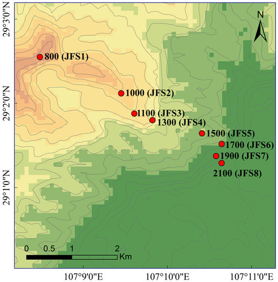
Figure 1.
Study area and sample locations.
Soil sampling was completed in October 2020, and promptly transported back to the lab in an ice cooler box. The fresh soil samples were sieved through a 2 mm sieve to remove stones, fine roots, and other residues. After homogenization, one part was kept at 4 °C for the soil physicochemical properties analysis, and the other part was stored at −80 °C for soil fungal community diversity studies.
2.3. Soil Analysis
2.3.1. Soil Physicochemical and Biological Properties
Soil bulk density (BD) was determined using the core cutter method with aluminum cans (31.4 cm3) as the sampling tool. Soil temperature at each altitude gradient was measured using a temperature sensor (HOBO H8 Pro, Onset Complete Corp., Bourne, MA, USA) and recorded every 30 min throughout the year. The soil particle size distribution was analyzed using the particle size analyzer (Mastersizer 2000, Malvern Instruments Ltd., UK). The soil pH was measured using a pH-meter (PHS-3C, SFMIT, Shanghai, China) with a soil-to-water ratio of 1:2.5. The soil organic carbon (SOC) and total nitrogen (TN) content were determined using the J200 Tandem laser spectroscopic element analyzer (Vario EL III; Elementar, Hanau, Germany), and their stocks were calculated using the formula provided by Guo and Gifford [44]. The soil fungal community diversity of each site was measured using the Illumina MiSeq sequencing method. We used the PowerSoilR DNA Isolation Kit (Axygen Biosciences, Union City, CA, U.S.) to extract microbial DNA from the −80 °C subsample soils according to the manufacturer’s instructions, and selected 3F_4R as the primer for the fungal ITS gene amplification. The purified PCR products from each sample were sequenced on the Illumina MiSeq platform in Shanghai. The diversity of soil fungal communities was represented by the Faith’s phylogenetic diversity (PD), species richness (Chao 1), and community coverage (Coverage).
2.3.2. Soil Aggregate Stability and Soil Erodibility
After air-drying, we broke the undisturbed soils into nearly 1 cm fractions along their natural cracks, and divided them into six sizes (>5, 2–5, 1–2, 0.5–1, 0.25–0.5, and <0.25 mm) using the dry sieve method. Based on the proportion of each aggregate size, we configured the 50 g soil samples, comprising different aggregate fractions. Then, we placed the soil samples in the soil aggregate analyzer, which was immersed in water and vibrated up and down, with a 35 mm amplitude and 25 times/min vibration frequency for 30 min. The water-stable aggregates of each size fraction (>2, 1–2, 0.5–1, 0.25–0.5, 0.106–0.25, and <0.106 mm) were collected and dried to constant weight at 60 °C. The soil aggregate stability was quantified by mean weight diameter (MWD), geometric mean diameter (GMD), fractal dimension (D), and the content of greater than 0.25 mm water-stable aggregates (R0.25), soil erodibility (k) estimated by the erosion productivity impact calculator (EPIC), and the Dg model [23,24,45]:
where wi is the proportion of the ith-size aggregate (%), xi is the mean diameter of the ith-size aggregate (mm), Xm is the diameter of the largest aggregate size (mm), w is the cumulative mass of less than ith-size aggregate (g), Mr>0.25 is the mass of greater than 0.25 mm aggregates (g), MT is the mass of the sample, CLA is the clay (%), SIL is the silt (%), SAN is the sand (%), and SNI is the 1-SAN (%).
2.3.3. Soil Quality Index
The procedure of developing an SQI using the minimum data set (MDS) method typically includes three main steps. Firstly, we performed the principal component analysis to select the most representative soil indicators for MDS. According to Andrews and Carroll [46], only principal components (PCs) with eigenvalues ≥1 and that explained at least 5% of the data variation were considered for the final MDS. In each PC, soil indicators with an absolute loading value ≥0.5 ware considered as highly weighted, and were divided into one group; if the indicator’s absolute loading value was ≥0.5 on multiple PCs, the indicator should be assigned to the group with the lowest correlation [47]. Then, we calculated the norm value of each indicator according to the formula provided by Yemefack et al. [6], and selected the indicators whose norm value was within 10% of the highest norm value of each group as the final MDS. The formula for calculating norm value is as follows:
where Nik is the comprehensive loading of the ith indicator on the first k PCs with eigenvalues of >1, uik is the loading of the ith indicator on the kth PC, and is the eigenvalue of the kth PC.
Secondly, we used the standard scoring functions to transfer the MDS indicators into a normalized value between 0 and 1 [48]. In general, there are three types of score functions: “more is better”, “less is better”, or “optimum”, and the selection of score function depended on whether a high value of the soil property was considered “good” or “bad” for soil function. The “more is better” (Equation (8)) and “less is better” (Equation (9)) scoring functions are as follows:
where f(x) is the score of the soil indicator; U and L are the upper and lower threshold values of the indicator, respectively; and x is the indicator value.
Thirdly, we used the communality of PCA to calculate the weight value of each MDS indicator, which is equal to the quotient of the communality divided by the sum of communalities of MDS indicators [9]. After scoring and weighting the soil indicators of the MDS, the integrated SQI was calculated using the following formula [46]:
where Wi is the weight value of the ith indicator, Si is the score of the ith indicator, and n is the number of indicators in MDS.
2.4. Statistical Analysis
One-way analysis of variance (ANOVA) and Fisher’s least significant difference (LSD) test were conducted to examine the effect of altitude gradient on soil properties, and significance was established at p < 0.05. Principal component analysis was performed to extract the representative soil indicators for MDS. Pearson’s correlation analysis was used to identify the correlation between the soil quality indicators. Stepwise regression analysis was used to assess the explanatory power of the soil variables on the variability of soil aggregate stability and k factors. Linear regression analysis was used to explore the quantitative relationship between the soil aggregate stability, k factor, and SQI; draw the best-fit lines; and determine the coefficient of R2 and the p-values. All of the statistical analyses were performed using SPSS 18.0 software (SPSS Incorporation, Chicago, IL, USA), and graphics were plotted using Origin 2023 software.
3. Results
3.1. Soil Physicochemical and Biological Properties
The soil BD ranged from 0.38 to 1.28 g cm−3, and the values of JFS2 and JFS3 were significantly higher than those of the other altitudes (p < 0.05) (Table 1). The soil temperature ranged from 4.79 to 11.64 °C and decreased linearly with the increase in altitude. Soil particle size distribution analysis showed that the proportion of clay (21.49%–40.71%), silt (25.85%–38.68%), and sand (26.59%–47.19%) was similar among the altitude gradients, but the macro-aggregate (0.06%–0.51%) had the lowest fraction (Table 1 and Figure 2).

Table 1.
Basic characteristics of each sampling site (mean ± SD, n = 4).
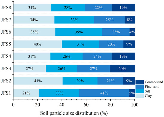
Figure 2.
Changes in soil particle size distribution across the altitude gradients on Jinfo mountain.
The soil pH was acidic-neutral, and the mean values ranged from 3.85 to 7.0 (Table 1). The contents of SOC ranged from 34.8 to 158 g kg−1, while those of TN ranged from 3.8 to 10.9 g kg−1 (Table 1). The SOC and TN at JFS4 were the highest, and were significantly higher than those of the other altitudes (p < 0.05). Except for JFS4, the SOC, TN, and C:N ratio showed a generally increased trend. The ranges of SOC and N stocks were 43.6–60.7 Mg ha−1 and 4.3–5.9 Mg ha−1, respectively; there were no significant differences among the altitudinal gradients (Table 1).
Faith’s phylogenetic diversity (PD) and Chao 1 species richness of the soil fungal communities at JFS6 were the highest, and the diversity indexes of JFS4, JFS7, and JFS8 were significantly lower than those of the other altitudes (p < 0.05) (Figure 3).
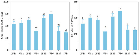
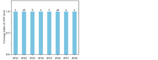
Figure 3.
Changes in soil fungal community diversity indexes across the altitude gradients on Jinfo mountain. Different letters represent significant differences across the altitude gradients at p < 0.05.
3.2. Soil Aggregate Stability and Soil Erodibility
The ranges of MWD, GMD, R0.25, and D were 1.21–1.77 mm, 0.72–1.43 mm, 70%–91%, and 2.11–2.71, respectively (Figure 4). In general, MWD, GMD, and R0.25 exhibited a unimodal altitudinal pattern, and reached the peak at JFS3 or JFS5. The D decreased initially and then increased with the increase in altitude gradient; the value of JFS3 was significantly lower than that of the other altitudes (p < 0.05).
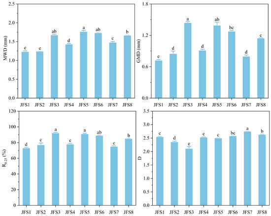
Figure 4.
Changes in soil aggregate stability across the altitude gradients on Jinfo mountain. MWD, mean weight diameter. GMD, geometric mean diameter. D, fractal dimension. R0.25, the percentage of greater than 0.25 mm water-stable aggregates. Different letters represent significant differences across the altitude gradients at p < 0.05.
The ranges of Kepic and KDg were 0.053–0.062 and 0.028–0.042, respectively (Figure 5). With the increase in altitude, KDg showed a decreasing trend, and the values of JFS1 and JFS2 were significantly higher than those of the other altitudes (p < 0.05). Kepic showed an S-shaped trend, but did not vary significantly, except for JFS6. In addition, stepwise regression analysis revealed that SOC, soil mechanical composition, BD, pH, temperature, and fungal community diversity are the major factors that explain the variability in soil aggregate stability and soil erodibility (Table 2).
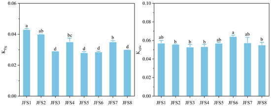
Figure 5.
Changes in soil erodibility (k) across altitude gradients on Jinfo mountain. KDg, the k factor of the Dg model. Kepic, the k factor of the EPIC model. Different letters represent significant differences across the altitude gradients at p < 0.05.
Table 2.
Stepwise regression analysis of the effect of soil properties on soil aggregate stability and soil erodibility (k).
3.3. Soil Quality Index
The first four PCs had eigenvalues of ≥1, and cumulatively explained 85.02% of the total variability (Table 3). SOC and the soil C:N ratio were both highly weighted indicators in PC1 and PC2, based on their correlation (Table A2), and SOC was assigned to group 1 and the soil C:N ratio assigned to group 2. Overall, the PD, Chao 1, soil pH, BD, Ns, and SOC were assigned to group 1, and PD had the highest norm value of 2.39, Chao 1 had a norm value within 10% of the highest value. However, PD correlated well with Chao 1 (correlation coefficient ≥ 0.6), thus, Chao 1 was removed. The TN and C:N ratio were assigned to group 2, and only the C:N ratio had the highest norm value of 2.09. The coverage and coarse sand were assigned to group 3, and their norm values were both within 10% of the highest value. MA was assigned to group 4. In summary, PD, coverage, coarse sand, C:N ratio, and MA were selected into final MDS, and their weight values were 0.19, 0.22, 0.26, 0.23, and 0.09, respectively (Table 3). The integrated SQI is given below: SQI = 0.19 × PD (S) + 0.22 × Coverage (S) + 0.26 × Coarse sand (S) + 0.09 × MA (S) + 0.23 × C:N ratio (S), where S is the score of the soil indicator in Equations (8) and (9).
Table 3.
Principal component analysis of the soil quality indicators.
The integrated values of SQI ranged from 0.30 to 0.62, and showed a unimodal altitudinal pattern, with a peak at JFS3 (Figure 6). In general, the soil quality of JFS2 and JFS3 was the best, followed by JFS8, JFS1, JFS4, and JFS5, and JFS6 and JFS7 which were the worst.
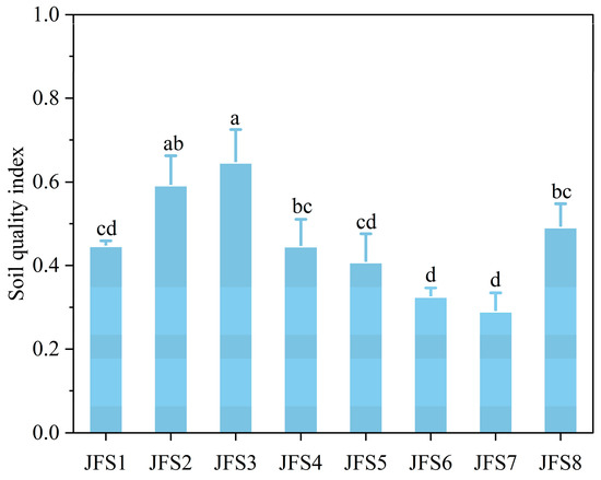
Figure 6.
Changes in SQI across altitude gradients on Jinfo mountain. Different letters represent significant differences across the altitude gradients at p < 0.05.
3.4. Effects of Fractal Dimension and Soil Erodibility on Soil Quality
The linear regression analysis indicated that SQI is significantly correlated with fractal dimension (D) (SQI = –0.5142D + 1.7318, R2 = 0.5980, p < 0.001) and the k factor of the EPIC model (Kepic) (SQI = –20.9617Kepic + 1.6327, R2 = 0.4573, p < 0.001) (Figure 7).
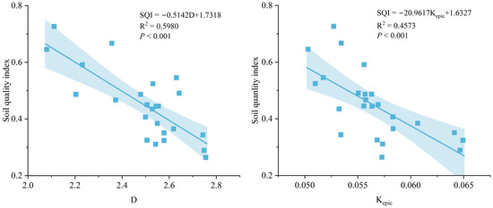
Figure 7.
The relationships between soil aggregate stability, soil erodibility, and SQI. D, fractal dimension. Kepic, the k factor of the EPIC model.
4. Discussion
4.1. Effects of Altitudinal Gradients on SOC, TN, and Fungal Community Diversity
Changes in altitude can create a gradient in the abiotic components, including temperature, humidity, and solar radiation, which in turn affect soil carbon and nitrogen dynamics [49]. Overall, the distribution of SOC and TN over altitudinal gradients both showed unimodal patterns (Table 1), which is consistent with the results of previous studies [50,51]. However, the SOC content at site JFS4 was anomalously higher than at the other sites (Table 1). There are two possible reasons to explain this result: (1) its overly acidic soil constrained soil microbial growth and extracellular enzyme activities, which in turn limited the decomposition process of organic material [52]; (2) its low bulk density favor enhanced root growth and led to SOC accumulation [53]. SOC and TN stocks showed a unimodal distribution pattern across the altitudinal gradients (Figure 1), which is inconsistent with a meta-analysis reporting a predictable increasing trend in SOC and TN stocks across the altitudinal gradient by Dieleman et al. [54]. This difference is mainly due to the significant fluctuations in soil BD (Table 1), which is the key parameter in the calculation of SOC and TN stocks [44]. In addition, a low soil temperature limited the cycling of organic matter [55], which may also have contributed to the higher contents of SOC and TN in high-altitude soils.
Soil fungal diversity showed a bimodal altitudinal pattern (Figure 3), which was inconsistent with previous reports of monotony decline, U-shaped, or no clear altitudinal patterns [39,56,57]. This is mainly because soil pH controlled the distribution pattern of soil fungal communities; their diversity indexes (Chao 1 and PD) are significantly positive correlated with soil pH (Table A1). Liu et al. found consistent results in a similar study area, and indicated that soil pH dominated species richness and Faith’s PD of soil fungal communities (R2 = 0.32 and 0.26, respectively) based on a DistLM analysis [39]. A controlled laboratory experiment also noted that a lower pH (pH < 4) could support the maintenance rather than flourishing of soil microbial communities [58]. Therefore, soil pH is recognized to be a universal predictor of soil fungal community distribution patterns. On Jinfo mountain, the soil parent rocks of different altitudes are inconsistent [41], which may be the main reason for the variation in soil pH, and thereby the significantly differences in soil fungal diversity. In addition, the C:N ratio was also significantly correlated with the soil fungal diversity indices (Table A1). This is mainly because the litter composition (C:N ratio) of plants can affect fungal growth during decomposition [59].
4.2. Effects of Altitudinal Gradients on Soil Aggregate Stability and Soil Erodibility
The soil aggregate stability exhibited a unimodal altitudinal pattern (Figure 4), which is inconsistent with a previous report in Helan Mountains [17], which found that the proportion of MA and MWD increased significantly along the altitudinal gradient. The difference in results is mainly attributed to the different study areas and objects; for example, these studies focused on arid mountain forest soils and restored cut slope soils [17,60]. Another possible reason is the higher biodiversity in the mid-altitudes of Jinfo mountain, which leads to a higher soil aggregate stability [61]. In this study, soil mechanical composition and soil fungal diversity provided the greatest explanatory power for the variations in MWD, GMD, R0.25, and D (Table 2). This is because soil fungal communities are the most important biological factors in soil aggregation, which can increase the stability of soil aggregates through the mechanical entanglement of soil particles by mycelium, and produce effective binding agents through the synthesis or decomposition of organic materials [15,62,63]. However, there was no positive relationship between SOC and soil aggregate stability (Table A1), which was inconsistent with previous results, because SOC is considered a major binding agent of soil aggregation [64]. The main reason is that in a karst mountainous area, low pH soil is rich in oxides, clay particles, and iron-aluminum oxides contents contribute more than SOC to the formation and stabilization of soil aggregates in oxide soils [65].
Soil erodibility (k) is a critical factor of soil erosion prediction in RUSLE. The mathematical model (EPIC and Dg) for calculating the k factor is mainly derived based on intrinsic soil properties [66]. Zhu et al. stated that there is no heterogeneity between the Dg model and EPIC model [25], which is inconsistent with the results of our study (Figure 5). This difference is mainly because the different estimation models focus on different soil properties, such as the EPIC model, which focused on the soil particles and SOC content, whereas the Dg model focused on the GMD of soil aggregates [23,24]. Overall, the estimated k values in this study were higher than that in the black soil region of northeast China (0.0105–0.0112 of the EPIC model), and similar to that in the Loess Plateau in northwest China (0.032–0.060 of the EPIC model and 0.018–0.044 of the Dg model) [22,67]. These results indicate that there are high erosion risks at all altitudinal gradients of a karst mountainous area. In addition, as the estimated data of k factor, soil mechanical composition explained the greatest variability in soil erodibility (Table 2). Soil fungal community diversity also had a higher weight that because of soil fungal communities can promote soil aggregation, which in turn increases the soil’s resistance to erosion [26].
4.3. Effects of Altitudinal Gradients on Soil Quality Index and Indicators
In this study, 5 of the 11 potential soil indicators were selected using the MDS method (Table 3). MDS comprised soil physical, chemical, and biological indicators, which is consistent with the results of previous studies [7,68]. The PD and coverage indexes of the soil fungal community are novel soil biological indicators [2] that are highly sensitive to changes in the external environment, and play an important role in soil biochemical processes [59]. In addition, they are closely related to soil pH and aggregate stability (Table A1). The soil C:N ratio is a critical chemical indicator, which not only reflects the combined effects of SOC and TN cycles, but also could influence soil microbial community structure [69]. Thus, soil C:N ratio is suitable as an indicator for soil quality assessment. Coarse sand and MA as the soil physical indicators were shown to have a significant effect on soil nutrients [70], and thus they were selected for developing the SQI.
The SQI exhibited a unimodal altitudinal pattern (Figure 6), which was inconsistent with a previous study on Mount Tai in the North China Plain that reported that the SQI showed an increasing trend with altitude [68]. This result suggests that altitude is not the major limiting factor of soil quality in karst mountainous area. In this study, the JFS3 site had the highest SQI value, probably because it had the highest soil aggregate stability and a relatively higher soil fungal diversity, SOC, and TN stocks. JFS7 had the lowest SQI value, possibly because it had a much lower soil pH, fungal diversity, and aggregate stability. Previous studies have indicated that the SOC content is the key factor affecting soil quality [40,70]. However, the JFS4 site had the highest SOC content, as well as a low soil BD, but had a lower SQI value. This may be due to its extremely acidic soil environment, which limited the diversity and activity of the soil microorganisms (Table 1 and Figure 3), thus leading to a decrease in soil quality. As an important part of soil, soil microorganisms actively participate in various biochemical processes of soil, and play a vital role in maintaining the structure and function of soil ecosystem [52,64]. Therefore, soil fungal community diversity, pH, C:N ratio, and mechanical composition are the key factors limiting soil quality in karst mountainous areas.
4.4. Effects of Fractal Dimension and Soil Erodibility on Soil Quality
In this study, D and Kepic showed a significant linear relationship with SQI (Figure 7). Stable soil structures typically have high nutrient levels, are less susceptible to soil erosion, and can harbor more stable soil microbial communities [71,72]. D can represent soil quality more accurately than MWD, GMD, and R0.25 (Figure 7). Similarly, Tagar et al. stated that D can be used as a dependable indicator of soil quality and has advantages over MWD [73]. There are three possible reasons for this result: (1) the information carried by MWD, GMD, and R0.25 is similar and simple, and an increase in their values represents an increase in the large-size aggregate content [74], while D not only contains information on soil aggregate size distribution, but also reflects soil moisture and other physical properties [75]. (2) D is developed from the fractal geometry theory, and has a strong theoretical foundation [76]. Soil’s geometric features, such as the arrangement of particles and pores, can be more easily captured by D [77]. (3) Compared with MWD, GMD, and R0.25, D is more sensitive to the changes in soil management [78] and is more appropriate for the analysis of field soils [74]. Additionally, D had a positive intrinsic correlation with Kepic [79] (Table A1), and Kepic can more accurately reflect the soil quality than KDg (Figure 7). This result attributed to GMD being the sole input parameter in the Dg model, which carries limited information about the soil properties. On the other hand, the k factor of the EPIC model, which is mainly controlled by the silt and SOC content [80,81], encompasses a broader range of soil physicochemical properties and thus provides a more comprehensive characterization of soil quality.
4.5. Limitations
This study enriched the results of soil properties’ response to climate change, and provided a novel method for rapid soil quality monitoring and assessment in karst mountainous areas. However, there were also some limitations. Firstly, the causal relationships among soil properties, such as the influence of soil pH on fungal community diversity and its contribution to SOC and TN accumulation, were primarily established based on correlation analysis and previous researches findings. Further confirmation through controlled laboratory experiments is necessary to validate these relationships. Secondly, apart from surface erosion, the unique double hydrogeological structure of the southwest karst area also involves underground leakage loss, which is an important pathway for soil loss. When sloping soil flows into underground space through continuous cracks, pipes, and holes, it leads to a high soil leakage ratio. This situation may render the soil erodibility of the EPIC model (Kepic) less applicable [82,83]. Thirdly, relying solely on D or Kepic as indicators of soil quality may be susceptible to random errors, consequently impacting the accuracy of the results. Therefore, it is recommended to incorporate other relevant soil parameters in conjunction with D or Kepic to achieve a more comprehensive and accurate assessment and monitoring of soil quality [10].
5. Conclusions
This research explored the effects of fractal dimension (D) and soil erodibility on soil quality in karst mountainous areas. The results showed the following: (1) Altitude exerted a significant influence on climate, soil pH, and fungal communities, and the accumulation of SOC, TN, and their stocks. (2) Key factors limiting soil quality were found to be soil mechanical composition, fungal diversity, pH, and C:N ratio. (3) SQI showed a significantly linear relationship with the fractal dimension (D) and soil erodibility (Kepic), suggesting that D and Kepic can be used as alternative indicators of soil quality. These single indicators cover a wide range of soil information, and can effectively characterize soil health, which is of great significance for guiding soil quality improvement and rocky desertification control. In addition, by employing these alternative indicators, the cost of the soil quality assessment can be reduced. Soil quality serves as the foundation for soil functions and ecosystem services; these results offer a scientific basis for soil erosion management and biodiversity conservation in karst mountainous areas. However, these findings were mainly based on the conclusion of correlations, where causality needs to be further verified by conducting subsequent relevant experiments.
Author Contributions
Conceptualization, G.Z. and D.L.; Methodology, X.H. and G.Z.; Validation, P.W. and L.Z. (Liang Zhao); Formal analysis, Y.L. and S.Q.; Investigation, L.Z. (Lihua Zhou), L.Z. (Lian Zeng) and G.Z.; Resources, Y.Y.; Writing original draft, Y.L. All authors have read and agreed to the published version of the manuscript.
Funding
This research was funded by the fellowship of the China Postdoctoral Science Foundation (2020M683235), and the Postdoctoral Science Foundation of Chongqing Natural Science Foundation (cstc2020jcyj-bshX0029).
Data Availability Statement
Data will be made available on request.
Acknowledgments
Financial support of this study was provided by the fellowship of the China Postdoctoral Science Foundation (2020M683235), and the Postdoctoral Science Foundation of Chongqing Natural Science Foundation (cstc2020jcyj-bshX0029).
Conflicts of Interest
The authors declare no conflict of interest.
Appendix A
Table A1.
Pearson’s correlation coefficients between soil properties, soil aggregate stability, and soil erodibility.
Table A1.
Pearson’s correlation coefficients between soil properties, soil aggregate stability, and soil erodibility.
| MWD | R0.25 | GMD | D | KDg | Kepic | TN | SOC | C:N Ratio | Ns | Cs | BD | pH | T | Chao 1 | PD | Coverage | |
|---|---|---|---|---|---|---|---|---|---|---|---|---|---|---|---|---|---|
| MWD | 1 | 0.896 ** | 0.892 ** | −0.012 | −0.984 ** | 0.174 | 0.208 | 0.105 | 0.045 | 0.307 | 0.267 | −0.107 | 0.083 | −0.637 ** | 0.337 | 0.28 | −0.074 |
| R0.25 | 1 | 0.986 ** | −0.415 * | −0.913 ** | 0.009 | 0.003 | −0.12 | −0.253 | 0.436 * | 0.187 | 0.258 | 0.237 | −0.322 | 0.487 * | 0.416 * | −0.207 | |
| GMD | 1 | −0.439 * | −0.897 ** | 0.001 | 0.011 | −0.128 | −0.286 | 0.429 * | 0.163 | 0.257 | 0.287 | −0.272 | 0.511 * | 0.447 * | −0.252 | ||
| D | 1 | 0.081 | 0.413 * | 0.462 * | 0.494 * | 0.599 ** | −0.333 | 0.101 | −0.780 ** | −0.258 | −0.611 ** | −0.369 | −0.313 | 0.500 * | |||
| KDg | 1 | −0.107 | −0.191 | −0.113 | −0.066 | −0.327 | −0.294 | 0.088 | 0.005 | 0.628 ** | −0.291 | −0.228 | 0.048 | ||||
| Kepic | 1 | 0.014 | −0.077 | −0.032 | 0.117 | 0.05 | −0.208 | 0.366 | −0.24 | 0.294 | 0.364 | 0.153 | |||||
| TN | 1 | 0.956 ** | 0.656 ** | 0.109 | 0.510 * | −0.574 ** | −0.102 | −0.352 | −0.08 | −0.128 | 0.362 | ||||||
| SOC | 1 | 0.828 ** | 0.032 | 0.555 ** | −0.632 ** | −0.332 | −0.37 | −0.255 | −0.315 | 0.364 | |||||||
| C:N ratio | 1 | −0.099 | 0.546 ** | −0.650 ** | −0.634 ** | −0.505 * | −0.498 * | −0.560 ** | 0.357 | ||||||||
| Ns | 1 | 0.767 ** | 0.306 | 0.225 | 0.032 | 0.627 ** | 0.536 ** | −0.071 | |||||||||
| Cs | 1 | −0.161 | −0.178 | −0.26 | 0.251 | 0.136 | 0.168 | ||||||||||
| BD | 1 | 0.455 * | 0.523 ** | 0.394 | 0.405 * | −0.326 | |||||||||||
| pH | 1 | 0.348 | 0.739 ** | 0.813 ** | −0.123 | ||||||||||||
| T | 1 | 0.233 | 0.221 | −0.189 | |||||||||||||
| Chao 1 | 1 | 0.968 ** | −0.406 * | ||||||||||||||
| PD | 1 | −0.335 | |||||||||||||||
| Coverage | 1 |
Notes: T, temperature; Cs, SOC stocks; Ns, nitrogen stocks; PD index, Chao1 index, coverage index, represent soil fungal community diversity; * p < 0.05; ** p < 0.01.
Table A2.
Pearson’s correlation coefficients between candidate soil quality indicators.
Table A2.
Pearson’s correlation coefficients between candidate soil quality indicators.
| TN | SOC | C:N Ratio | Ns | Soil BD | Soil pH | MA | Coarse Sand | Chao 1 | Coverage | PD | |
|---|---|---|---|---|---|---|---|---|---|---|---|
| TN | 1 | 0.956 ** | 0.656 ** | 0.109 | −0.574 ** | −0.102 | −0.311 | −0.037 | −0.08 | 0.362 | −0.128 |
| SOC | 1 | 0.828 ** | 0.032 | −0.632 ** | −0.332 | −0.322 | 0.027 | −0.255 | 0.364 | −0.315 | |
| C:N ratio | 1 | −0.099 | −0.650 ** | −0.634 ** | −0.478 * | 0.021 | −0.498 * | 0.357 | −0.560 ** | ||
| Ns | 1 | 0.306 | 0.225 | 0.076 | −0.214 | 0.627 ** | −0.071 | 0.536 ** | |||
| Soil BD | 1 | 0.455 * | 0.499 * | 0.077 | 0.394 | −0.326 | 0.405 * | ||||
| Soil pH | 1 | 0.219 | −0.326 | 0.739 ** | −0.123 | 0.813 ** | |||||
| MA | 1 | 0.137 | 0.07 | −0.135 | 0.098 | ||||||
| Coarse sand | 1 | −0.264 | −0.158 | −0.332 | |||||||
| Chao 1 | 1 | −0.406 * | 0.968 ** | ||||||||
| Coverage | 1 | −0.335 | |||||||||
| PD | 1 |
Notes: PD index, Chao1 index, coverage index, represent soil fungal community diversity; MA, macro-aggregate; Ns, nitrogen stocks; * p < 0.05; ** p < 0.01.
References
- Pimentel, D.; Harvey, C.; Resosudarmo, P.; Sinclair, K.; Kurz, D.; McNair, M.; Crist, S.; Shpritz, L.; Fitton, L.; Saffouri, R.; et al. Environmental and Economic Costs of Soil Erosion and Conservation Benefits. Science 1995, 267, 1117–1123. [Google Scholar] [CrossRef]
- Bünemann, E.K.; Bongiorno, G.; Bai, Z.; Creamer, R.E.; De Deyn, G.; de Goede, R.; Fleskens, L.; Geissen, V.; Kuyper, T.W.; Mäder, P.; et al. Soil quality—A critical review. Soil Biol. Biochem. 2018, 120, 105–125. [Google Scholar] [CrossRef]
- Doran, J.W.; Parkin, T.B. Defining and Assessing Soil Quality, Defining Soil Quality for a Sustainable Environment. In Defining Soil Quality for a Sustainable Environment; SSSA Special Publications; Coleman, D.C., Bezdicek, D.F., Stewart, B.A., Eds.; Wiley: Hoboken, NJ, USA, 1994; Volume 35, pp. 1–21. [Google Scholar]
- Andrews, S.S.; Karlen, D.L.; Mitchell, J.P. A comparison of soil quality indexing methods for vegetable production systems in Northern California. Agric. Ecosyst. Environ. 2002, 90, 25–45. [Google Scholar] [CrossRef]
- Yu, P.; Liu, S.; Zhang, L.; Li, Q.; Zhou, D. Selecting the minimum data set and quantitative soil quality indexing of alkaline soils under different land uses in northeastern China. Sci. Total Environ. 2018, 616–617, 564–571. [Google Scholar] [CrossRef]
- Yemefack, M.; Jetten, V.G.; Rossiter, D.G. Developing a minimum data set for characterizing soil dynamics in shifting cultivation systems. Soil Tillage Res. 2006, 86, 84–98. [Google Scholar] [CrossRef]
- Geng, S.; Shi, P.; Zong, N.; Zhu, W. Using Soil Survey Database to Assess Soil Quality in the Heterogeneous Taihang Mountains, North China. Sustainability 2018, 10, 3443. [Google Scholar] [CrossRef]
- Drobnik, T.; Greiner, L.; Keller, A.; Grêt-Regamey, A. Soil quality indicators—From soil functions to ecosystem services. Ecol. Indic. 2018, 94, 151–169. [Google Scholar] [CrossRef]
- Shukla, M.K.; Lal, R.; Ebinger, M. Determining soil quality indicators by factor analysis. Soil Till. Res. 2006, 87, 194–204. [Google Scholar] [CrossRef]
- Seybold, C.A.; Herrick, J.E. Aggregate stability kit for soil quality assessments. Catena 2001, 44, 37–45. [Google Scholar] [CrossRef]
- Ditzler, C. Erosion: Soil Quality. In Managing Soils and Terrestrial Systems; CRC Press: Boca Raton, FL, USA, 2020; pp. 153–156. [Google Scholar]
- Li, G.; Fu, Y.; Li, B.; Zheng, T.; Wu, F.; Peng, G.; Xiao, T. Micro-characteristics of soil aggregate breakdown under raindrop action. Catena 2018, 162, 354–359. [Google Scholar] [CrossRef]
- Amézketa, E. Soil Aggregate Stability: A Review. J. Sustain. Agric. 1999, 14, 83–151. [Google Scholar] [CrossRef]
- Rabot, E.; Wiesmeier, M.; Schlüter, S.; Vogel, H.-J. Soil structure as an indicator of soil functions: A review. Geoderma 2018, 314, 122–137. [Google Scholar] [CrossRef]
- Six, J.; Elliott, E.; Paustian, K. Soil macroaggregate turnover and microaggregate formation: A mechanism for C sequestration under no-tillage agriculture. Soil Biol. Biochem. 2000, 32, 2099–2103. [Google Scholar] [CrossRef]
- Dou, Y.; Yang, Y.; An, S.; Zhu, Z. Effects of different vegetation restoration measures on soil aggregate stability and erodibility on the Loess Plateau, China. Catena 2020, 185, 104294. [Google Scholar] [CrossRef]
- Wu, M.; Pang, D.; Chen, L.; Li, X.; Liu, L.; Liu, B.; Li, J.; Wang, J.; Ma, L. Chemical composition of soil organic carbon and aggregate stability along an elevation gradient in Helan Mountains, northwest China. Ecol. Indic. 2021, 131, 108228. [Google Scholar] [CrossRef]
- Paul, B.K.; Vanlauwe, B.; Ayuke, F.; Gassner, A.; Hoogmoed, M.; Hurisso, T.; Koala, S.; Lelei, D.; Ndabamenye, T.; Six, J.; et al. Medium-term impact of tillage and residue management on soil aggregate stability, soil carbon and crop productivity. Agric. Ecosyst. Environ. 2013, 164, 14–22. [Google Scholar] [CrossRef]
- Sarker, J.R.; Singh, B.P.; Cowie, A.L.; Fang, Y.; Collins, D.; Badgery, W.; Dalal, R.C. Agricultural management practices impacted carbon and nutrient concentrations in soil aggregates, with minimal influence on aggregate stability and total carbon and nutrient stocks in contrasting soils. Soil Tillage Res. 2018, 178, 209–223. [Google Scholar] [CrossRef]
- Totsche, K.U.; Amelung, W.; Gerzabek, M.H.; Guggenberger, G.; Klumpp, E.; Knief, C.; Lehndorff, E.; Mikutta, R.; Peth, S.; Prechtel, A.; et al. Microaggregates in soils. J. Plant Nutr. Soil Sci. 2018, 181, 104–136. [Google Scholar] [CrossRef]
- Liu, M.; Han, G.; Zhang, Q. Effects of Soil Aggregate Stability on Soil Organic Carbon and Nitrogen under Land Use Change in an Erodible Region in Southwest China. Int. J. Environ. Res. Public Health 2019, 16, 3809. [Google Scholar] [CrossRef]
- Zhao, W.; Wei, H.; Jia, L.; Daryanto, S.; Zhang, X.; Liu, Y. Soil erodibility and its influencing factors on the Loess Plateau of China: A case study in the Ansai watershed. Solid Earth 2018, 9, 1507–1516. [Google Scholar] [CrossRef]
- Shirazi, M.A.; Boersma, L.; Hart, J.W. A Unifying Quantitative Analysis of Soil Texture: Improvement of Precision and Extension of Scale. Soil Sci. Soc. Am. J. 1988, 52, 181–190. [Google Scholar] [CrossRef]
- Williams, J.R.; Renard, K.G.; Dyke, P.T. EPIC: A new method for assessing erosion’s effect on soil productivity. J. Soil Water Conserv. 1983, 38, 381–383. [Google Scholar]
- Zhu, G.; Tang, Z.; Shangguan, Z.; Peng, C.; Deng, L. Factors Affecting the Spatial and Temporal Variations in Soil Erodibility of China. J. Geophys. Res. Earth Surf. 2019, 124, 737–749. [Google Scholar] [CrossRef]
- Nciizah, A.D.; Wakindiki, I.I. Physical indicators of soil erosion, aggregate stability and erodibility. Arch. Agron. Soil Sci. 2014, 61, 827–842. [Google Scholar] [CrossRef]
- Wang, K.; Zhang, C.; Chen, H.; Yue, Y.; Zhang, W.; Zhang, M.; Qi, X.; Fu, Z. Karst landscapes of China: Patterns, ecosystem processes and services. Landsc. Ecol. 2019, 34, 2743–2763. [Google Scholar] [CrossRef]
- Jianhua, C.; Daoxian, Y.; Liqiang, T.; Mallik, A.; Hui, Y.; Fen, H. An Overview of Karst Ecosystem in Southwest China: Current State and Future Management. J. Resour. Ecol. 2015, 6, 247–256. [Google Scholar] [CrossRef]
- Banks, D.; Odling, N.E.; Skarphagen, H.; Rohr-Torp, E. Permeability and stress in crystalline rocks. Terra Nova 1996, 8, 223–235. [Google Scholar] [CrossRef]
- Manoutsoglou, E.; Lazos, I.; Steiakakis, E.; Vafeidis, A. The Geomorphological and Geological Structure of the Samaria Gorge, Crete, Greece—Geological Models Comprehensive Review and the Link with the Geomorphological Evolution. Appl. Sci. 2022, 12, 10670. [Google Scholar] [CrossRef]
- Bucher, S. Origin of salinity of deep groundwater in crystalline rocks. Terra Nova 1999, 11, 181–185. [Google Scholar] [CrossRef]
- Huang, Q.; Cai, Y.; Xing, X. Rocky desertification, antidesertification, and sustainable development in the karst mountain region of Southwest China. AMBIO A J. Hum. Environ. 2008, 37, 390–392. [Google Scholar] [CrossRef]
- Dai, Q.; Liu, Z.; Shao, H.; Yang, Z. Karst bare slope soil erosion and soil quality: A simulation case study. Solid Earth 2015, 6, 985–995. [Google Scholar] [CrossRef]
- Thomas, J.; Joseph, S.; Thrivikramji, K.P. Assessment of soil erosion in a monsoon-dominated mountain river basin in India using RUSLE-SDR and AHP. Hydrol. Sci. J. 2018, 63, 542–560. [Google Scholar] [CrossRef]
- Lan, J.; Long, Q.; Huang, M.; Jiang, Y.; Hu, N. Afforestation-induced large macroaggregate formation promotes soil organic carbon accumulation in degraded karst area. For. Ecol. Manag. 2022, 505, 119884. [Google Scholar] [CrossRef]
- Arunrat, N.; Sereenonchai, S.; Kongsurakan, P.; Hatano, R. Assessing Soil Organic Carbon, Soil Nutrients and Soil Erodibility under Terraced Paddy Fields and Upland Rice in Northern Thailand. Agronomy 2022, 12, 537. [Google Scholar] [CrossRef]
- Zhang, Y.; Xu, X.; Li, Z.; Liu, M.; Xu, C.; Zhang, R.; Luo, W. Effects of vegetation restoration on soil quality in degraded karst landscapes of southwest China. Sci. Total. Environ. 2019, 650, 2657–2665. [Google Scholar] [CrossRef] [PubMed]
- Peng, X.; Wang, X.; Dai, Q.; Ding, G.; Li, C. Soil structure and nutrient contents in underground fissures in a rock-mantled slope in the karst rocky desertification area. Environ. Earth Sci. 2020, 79, 3. [Google Scholar] [CrossRef]
- Liu, D.; Liu, G.; Chen, L.; Wang, J.; Zhang, L. Soil pH determines fungal diversity along an elevation gradient in Southwestern China. Sci. China Life Sci. 2018, 61, 718–726. [Google Scholar] [CrossRef]
- Zhang, J.; Chen, H.; Fu, Z.; Wang, K. Effects of vegetation restoration on soil properties along an elevation gradient in the karst region of southwest China. Agric. Ecosyst. Environ. 2021, 320, 107572. [Google Scholar] [CrossRef]
- Zhu, G.; Zhou, L.; He, X.; Wei, P.; Lin, D.; Qian, S.; Zhao, L.; Luo, M.; Yin, X.; Zeng, L.; et al. Effects of Elevation Gradient on Soil Carbon and Nitrogen in a Typical Karst Region of Chongqing, Southwest China. J. Geophys. Res. Biogeosci. 2022, 127, e2021JG006742. [Google Scholar] [CrossRef]
- Zhang, C.; Yan, J.; Pei, J.; Jiang, Y. Hydrochemical variations of epikarst springs in vertical climate zones: A case study in Jinfo Mountain National Nature Reserve of China. Environ. Earth Sci. 2011, 63, 375–381. [Google Scholar] [CrossRef]
- Zhou, H.Y.; Pan, X.Y.; Zhou, W.Z. Assessing spatial distribution of soil erosion in a karst region in southwestern China: A case study in Jinfo Mountains. IOP Conf. Series: Earth Environ. Sci. 2017, 52, 012047. [Google Scholar] [CrossRef]
- Guo, L.B.; Gifford, R.M. Soil carbon stocks and land use change: A meta analysis. Glob. Chang. Biol. 2002, 8, 345–360. [Google Scholar] [CrossRef]
- Yang, P.; Luo, Y.; Shi, Y. Soil fractal characteristics characterized by the weight distribution of the particle size. Chin. Sci. Bull. 1993, 20, 1896–1899. (In Chinese) [Google Scholar]
- Andrews, S.S.; Carroll, C.R. Designing a soil quality assessment tool for sustainable agroecosystem management. Ecol Appl. 2001, 11, 1573–1585. [Google Scholar] [CrossRef]
- Li, G.; Chen, J.; Sun, Z.; Tan, M. Determination of minimum data set for soil quality assessment based on soil characteristics and land use change. Acta Ecol. Sin. 2007, 27, 2715–2724. (In Chinese) [Google Scholar] [CrossRef]
- Diack, M.; Stott, D.E. Development of a soil quality index for the Chalmers Silty Clay Loam from the Midwest USA. In Proceedings of the 10th International Soil Conservation Organization Meeting, West Lafayette, IN, USA, 24–29 May 1999; pp. 550–555. [Google Scholar]
- Tashi, S.; Singh, B.; Keitel, C.; Adams, M. Soil carbon and nitrogen stocks in forests along an altitudinal gradient in the eastern Himalayas and a meta-analysis of global data. Glob. Chang. Biol. 2016, 22, 2255–2268. [Google Scholar] [CrossRef]
- Li, C.; Cao, Z.; Chang, J.; Zhang, Y.; Zhu, G.; Zong, N.; He, Y.; Zhang, J.; He, N. Elevational gradient affect functional fractions of soil organic carbon and aggregates stability in a Tibetan alpine meadow. Catena 2017, 156, 139–148. [Google Scholar] [CrossRef]
- Schindlbacher, A.; de Gonzalo, C.; Díaz-Pinés, E.; Gorría, P.; Matthews, B.; Inclán, R.; Zechmeister-Boltenstern, S.; Rubio, A.; Jandl, R. Temperature sensitivity of forest soil organic matter decomposition along two elevation gradients. J. Geophys. Res. Atmos. 2010, 115, 3–18. [Google Scholar] [CrossRef]
- Stark, S.; Männistö, M.K.; Eskelinen, A. Nutrient availability and pH jointly constrain microbial extracellular enzyme activities in nutrient-poor tundra soils. Plant Soil 2014, 383, 373–385. [Google Scholar] [CrossRef]
- Davy, M.C.; Koen, T.B. Variations in soil organic carbon for two soil types and six land uses in the Murray Catchment, New South Wales, Australia. Soil Res. 2013, 51, 631–644. [Google Scholar] [CrossRef]
- Dieleman, W.I.; Venter, M.; Ramachandra, A.; Krockenberger, A.K.; Bird, M.I. Soil carbon stocks vary predictably with altitude in tropical forests: Implications for soil carbon storage. Geoderma 2013, 204–205, 59–67. [Google Scholar] [CrossRef]
- He, X.; Chu, C.; Yang, Y.; Shu, Z.; Li, B.; Hou, E. Bedrock and climate jointly control the phosphorus status of subtropical forests along two elevational gradients. Catena 2021, 206, 105525. [Google Scholar] [CrossRef]
- Shen, C.; Xiong, J.; Zhang, H.; Feng, Y.; Lin, X.; Li, X.; Liang, W.; Chu, H. Soil pH drives the spatial distribution of bacterial communities along elevation on Changbai Mountain. Soil Biol. Biochem. 2013, 57, 204–211. [Google Scholar] [CrossRef]
- Siles, J.A.; Margesin, R. Abundance and Diversity of Bacterial, Archaeal, and Fungal Communities Along an Altitudinal Gradient in Alpine Forest Soils: What Are the Driving Factors? Microb. Ecol. 2016, 72, 207–220. [Google Scholar] [CrossRef]
- Rousk, J.; Bååth, E.; Brookes, P.C.; Lauber, C.L.; Lozupone, C.; Caporaso, J.G.; Knight, R.; Fierer, N. Soil bacterial and fungal communities across a pH gradient in an arable soil. ISME J. 2010, 4, 1340–1351. [Google Scholar] [CrossRef]
- Grosso, F.; Bååth, E.; De Nicola, F. Bacterial and fungal growth on different plant litter in Mediterranean soils: Effects of C/N ratio and soil pH. Appl. Soil Ecol. 2016, 108, 1–7. [Google Scholar] [CrossRef]
- Zhu, M.; Yang, S.; Ai, S.; Ai, X.; Jiang, X.; Chen, J.; Li, R.; Ai, Y. Artificial soil nutrient, aggregate stability and soil quality index of restored cut slopes along altitude gradient in southwest China. Chemosphere 2020, 246, 125687. [Google Scholar] [CrossRef] [PubMed]
- Ma, S.Y.; Ma, J.L.; Wang, X.M. Jinfo Nature Reserve Scientific Investigation Report; Forestry Bureau of Chongqing Nanchuan: Chongqing, China, 1998; pp. 35–65. (In Chinese) [Google Scholar]
- Lynch, J.M.; Bragg, E. Microorganisms and Soil Aggregate Stability. In Advances in Soil Science; Springer: New York, NY, USA, 1985; pp. 133–171. [Google Scholar] [CrossRef]
- Tisdall, J.M.; Oades, J.M. Organic matter and water-stable aggregates in soils. Eur. J. Soil Sci. 1982, 33, 141–163. [Google Scholar] [CrossRef]
- Six, J.; Bossuyt, H.; Degryze, S.; Denef, K. A history of research on the link between (micro)aggregates, soil biota, and soil organic matter dynamics. Soil Tillage Res. 2004, 79, 7–31. [Google Scholar] [CrossRef]
- Jozefaciuk, G.; Czachor, H. Impact of organic matter, iron oxides, alumina, silica and drying on mechanical and water stability of artificial soil aggregates. Assessment of new method to study water stability. Geoderma 2014, 221–222, 1–10. [Google Scholar] [CrossRef]
- Gao, J.; Wang, H. Temporal analysis on quantitative attribution of karst soil erosion: A case study of a peak-cluster depression basin in Southwest China. Catena 2019, 172, 369–377. [Google Scholar] [CrossRef]
- Chen, S.; Zhang, G.; Zhu, P.; Wang, C.; Wan, Y. Impact of slope position on soil erodibility indicators in rolling hill regions of northeast China. Catena 2022, 217, 106475. [Google Scholar] [CrossRef]
- Shao, G.; Ai, J.; Sun, Q.; Hou, L.; Dong, Y. Soil quality assessment under different forest types in the Mount Tai, central Eastern China. Ecol. Indic. 2020, 115, 106439. [Google Scholar] [CrossRef]
- Dai, X.; Zhou, W.; Liu, G.; Liang, G.; He, P.; Liu, Z. Soil C/N and pH together as a comprehensive indicator for evaluating the effects of organic substitution management in subtropical paddy fields after application of high-quality amendments. Geoderma 2019, 337, 1116–1125. [Google Scholar] [CrossRef]
- Raiesi, F. A minimum data set and soil quality index to quantify the effect of land use conversion on soil quality and degradation in native rangelands of upland arid and semiarid regions. Ecol. Indic. 2017, 75, 307–320. [Google Scholar] [CrossRef]
- Nichols, K.; Toro, M. A whole soil stability index (WSSI) for evaluating soil aggregation. Soil Tillage Res. 2011, 111, 99–104. [Google Scholar] [CrossRef]
- Upton, R.N.; Bach, E.M.; Hofmockel, K.S. Spatio-temporal microbial community dynamics within soil aggregates. Soil Biol. Biochem. 2019, 132, 58–68. [Google Scholar] [CrossRef]
- Tagar, A.; Adamowski, J.; Memon, M.; Do, M.C.; Mashori, A.; Soomro, A.; Bhayo, W. Soil fragmentation and aggregate stability as affected by conventional tillage implements and relations with fractal dimensions. Soil Tillage Res. 2020, 197, 104494. [Google Scholar] [CrossRef]
- Pirmoradian, N.; Sepaskhah, A.; Hajabbasi, M. Application of Fractal Theory to quantify Soil Aggregate Stability as influenced by Tillage Treatments. Biosyst. Eng. 2005, 90, 227–234. [Google Scholar] [CrossRef]
- Pachepsky, Y.A.; Giménez, D.; Crawford, J.W.; Rawls, W.J. Conventional and fractal geometry in soil science. Dev. Soil Sci. 2000, 27, 7–18. [Google Scholar] [CrossRef]
- Bartoli, F.; Philippy, R.; Doirisse, M.; Niquet, S.; Dubuit, M. Structure and self-similarity in silty and sandy soils: The fractal approach. Eur. J. Soil Sci. 1991, 42, 167–185. [Google Scholar] [CrossRef]
- Caruso, T.; Barto, E.K.; Siddiky, R.K.; Smigelski, J.; Rillig, M.C. Are power laws that estimate fractal dimension a good descriptor of soil structure and its link to soil biological properties? Soil Biol. Biochem. 2011, 43, 359–366. [Google Scholar] [CrossRef]
- Gülser, C. Effect of forage cropping treatments on soil structure and relationships with fractal dimensions. Geoderma 2006, 131, 33–44. [Google Scholar] [CrossRef]
- Ahmadi, A.; Neyshabouri, M.-R.; Rouhipour, H.; Asadi, H. Fractal dimension of soil aggregates as an index of soil erodibility. J. Hydrol. 2011, 400, 305–311. [Google Scholar] [CrossRef]
- Arunrat, N.; Sereenonchai, S.; Kongsurakan, P.; Iwai, C.B.; Yuttitham, M.; Hatano, R. Post-fire recovery of soil organic carbon, soil total nitrogen, soil nutrients, and soil erodibility in rotational shifting cultivation in Northern Thailand. Front. Environ. Sci. 2023, 11, 1117427. [Google Scholar] [CrossRef]
- Huang, T.C.C.; Lo, K.F.A. Effects of Land Use Change on Sediment and Water Yields in Yang Ming Shan National Park, Taiwan. Environments 2015, 2, 32–42. [Google Scholar] [CrossRef]
- Wei, X.; Yan, Y.; Xie, D.; Ni, J.; Loáiciga, H.A. The soil leakage ratio in the Mudu watershed, China. Environ. Earth Sci. 2016, 75, 721. [Google Scholar] [CrossRef]
- Wang, J.; Zou, B.; Liu, Y.; Tang, Y.; Zhang, X.; Yang, P. Erosion-creep-collapse mechanism of underground soil loss for the karst rocky desertification in Chenqi village, Puding county, Guizhou, China. Environ. Earth Sci. 2014, 72, 2751–2764. [Google Scholar] [CrossRef]
Disclaimer/Publisher’s Note: The statements, opinions and data contained in all publications are solely those of the individual author(s) and contributor(s) and not of MDPI and/or the editor(s). MDPI and/or the editor(s) disclaim responsibility for any injury to people or property resulting from any ideas, methods, instructions or products referred to in the content. |
© 2023 by the authors. Licensee MDPI, Basel, Switzerland. This article is an open access article distributed under the terms and conditions of the Creative Commons Attribution (CC BY) license (https://creativecommons.org/licenses/by/4.0/).