

Transaction Costs and Investment Interest in the U.S. South and the Pacific Northwest Timberland Regions


Abstract
1. Introduction
1.1. Means of Investing in U.S. Timberland
1.2. Investing in the U.S. South vs. the Pacific Northwest
2. Materials and Methods
Hypothesis Testing
- In which U.S. regions do you invest, own, operate, or manage other’s timberland?
- Please rank by priority the region in the U.S. in which you are trying to invest capital in timberlands.
- Please rank by timberland region in the U.S. by the total transaction costs each requires to invest capital.
3. Results and Discussion
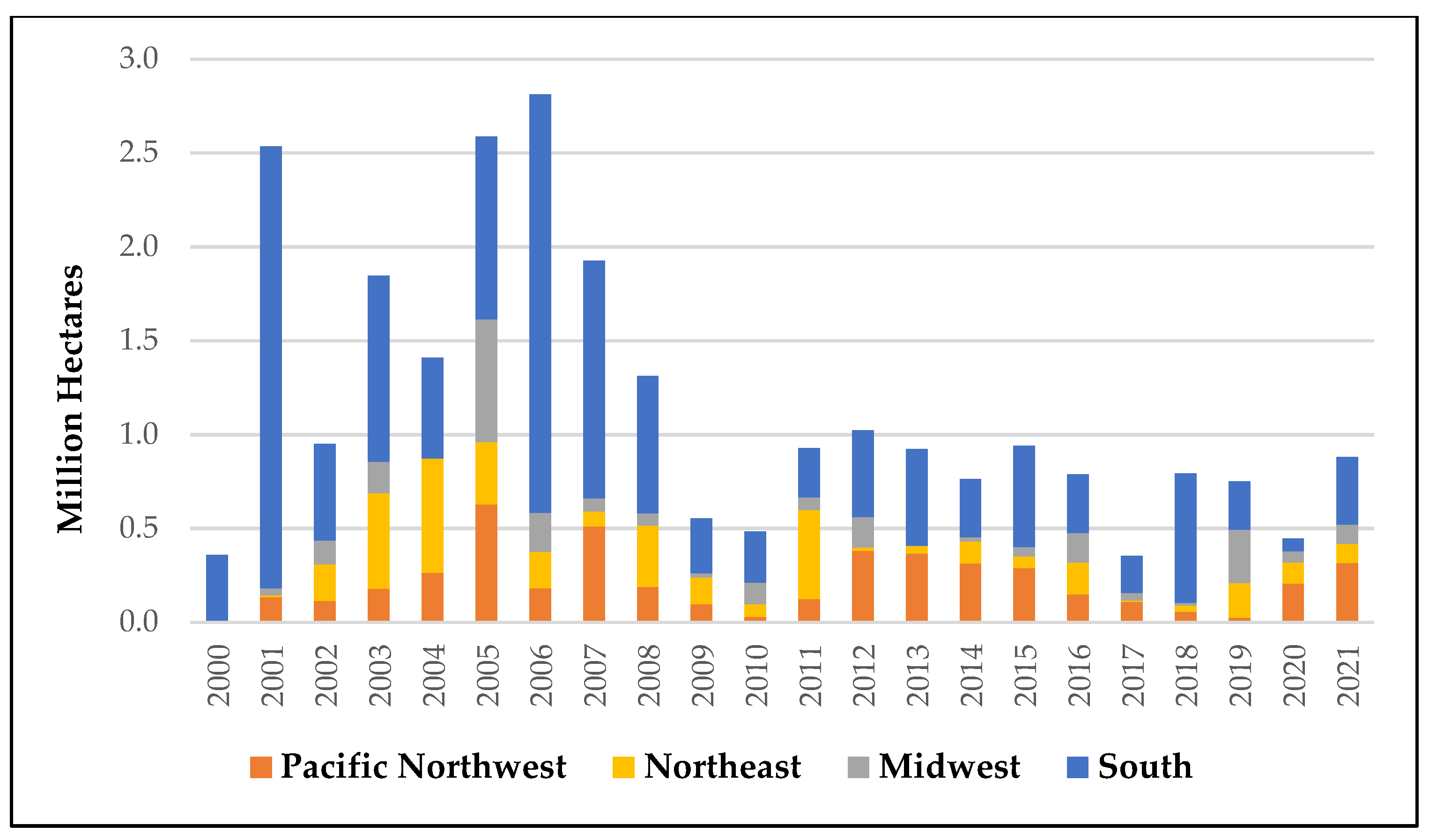
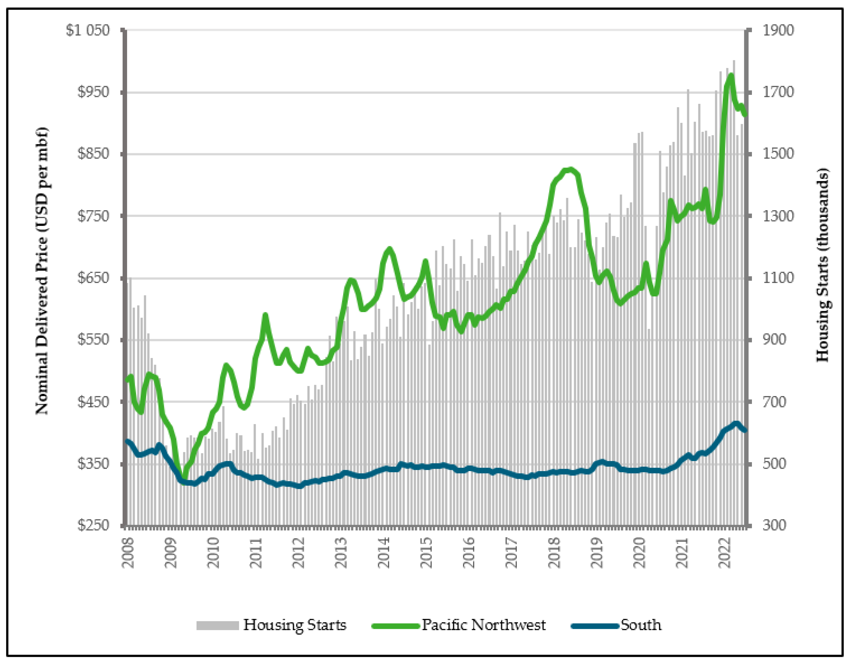
3.1. Timberland Transaction Data
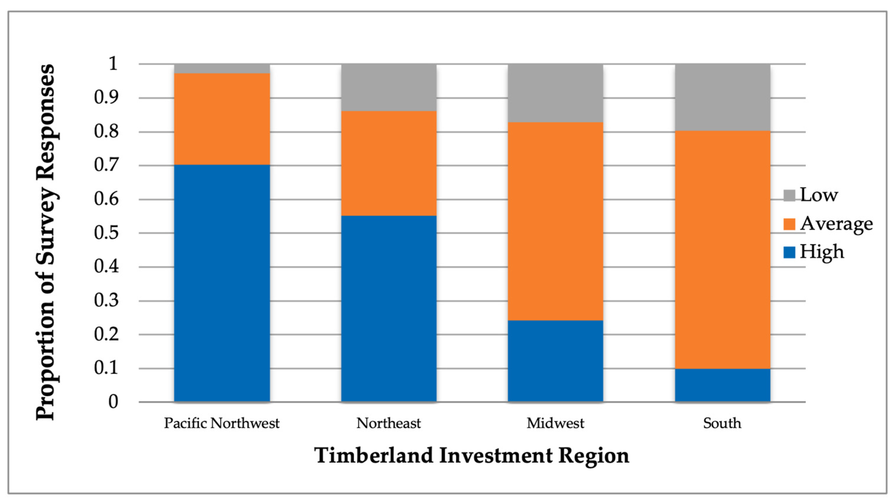
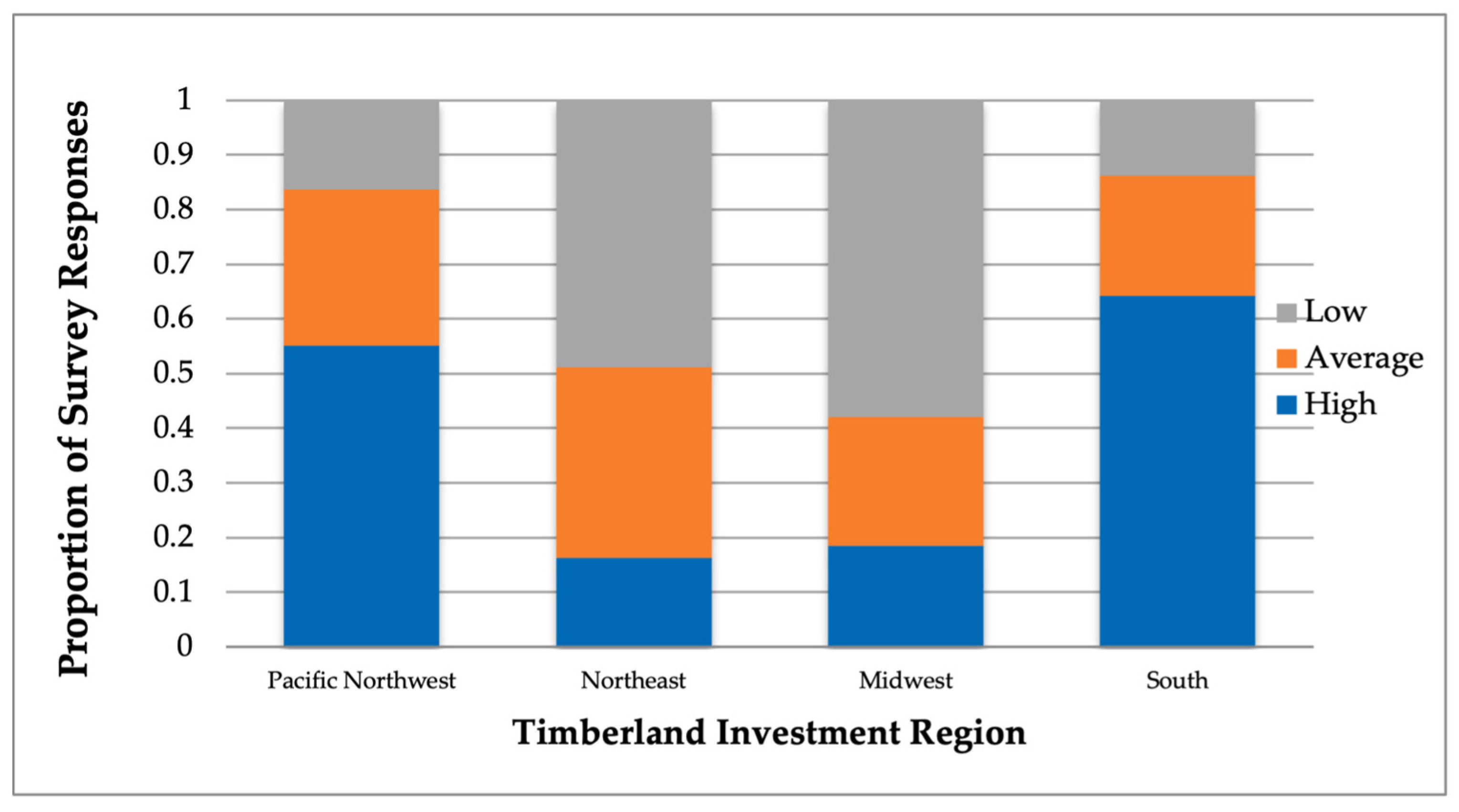
3.2. 2020 Timberland Transaction Cost Survey Results

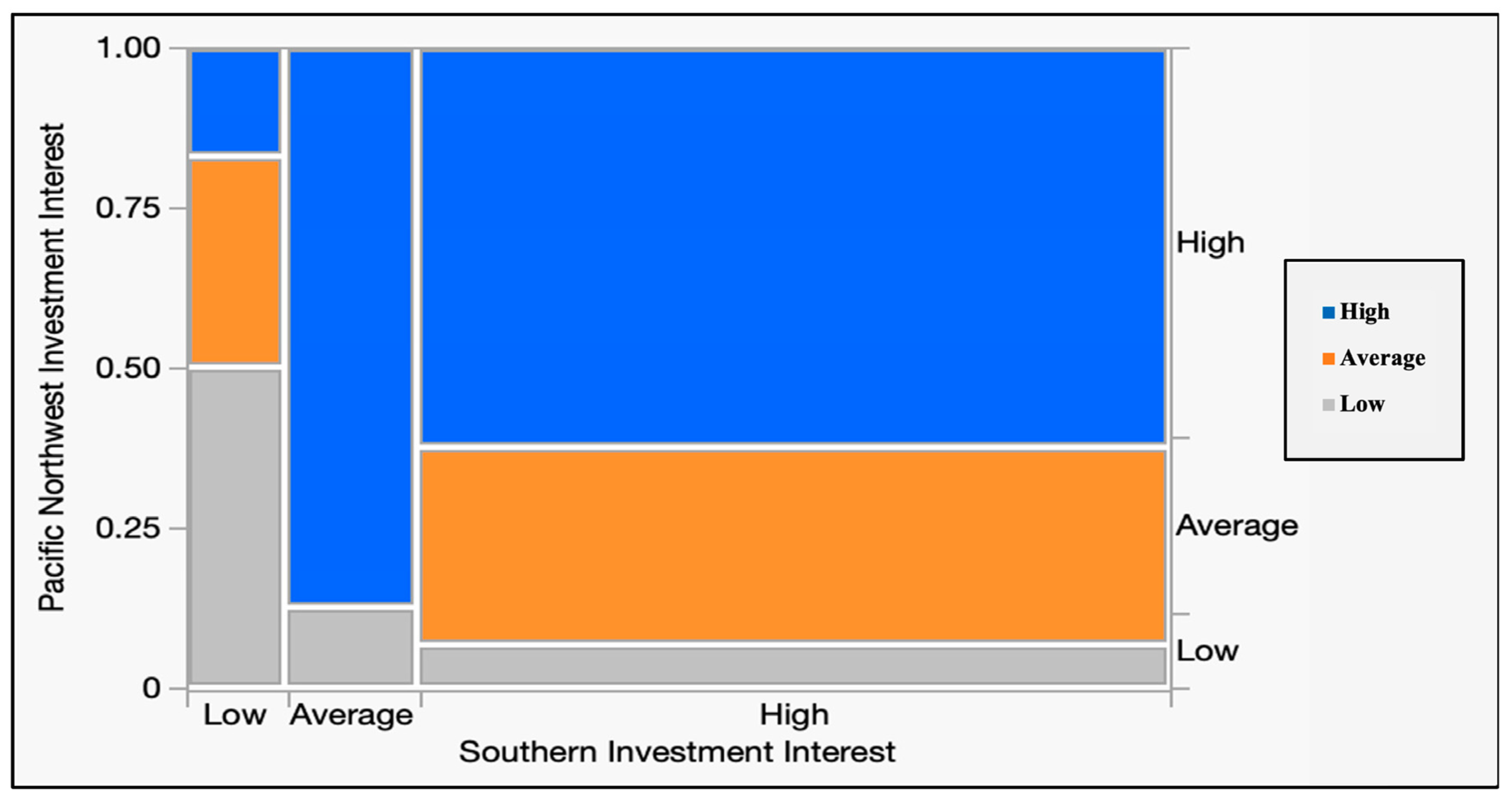
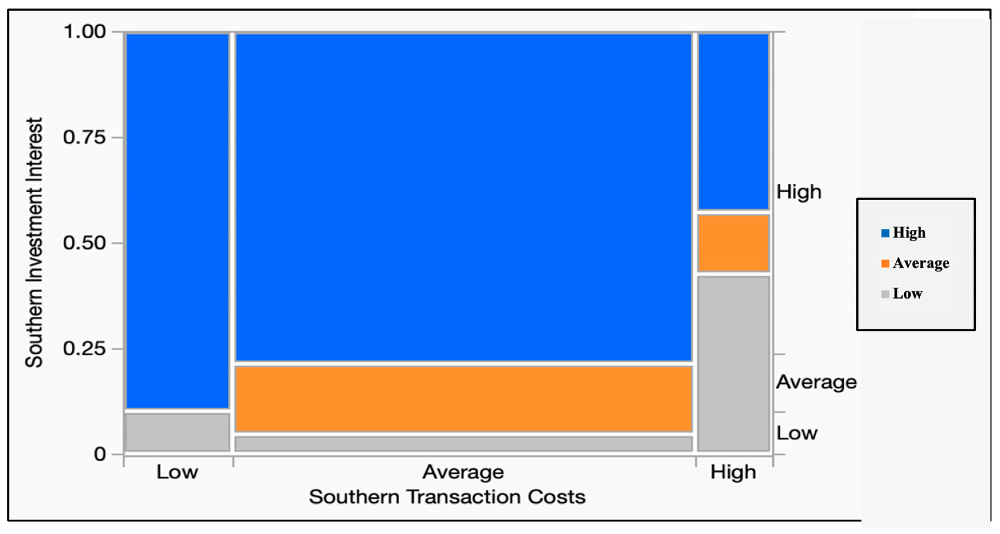
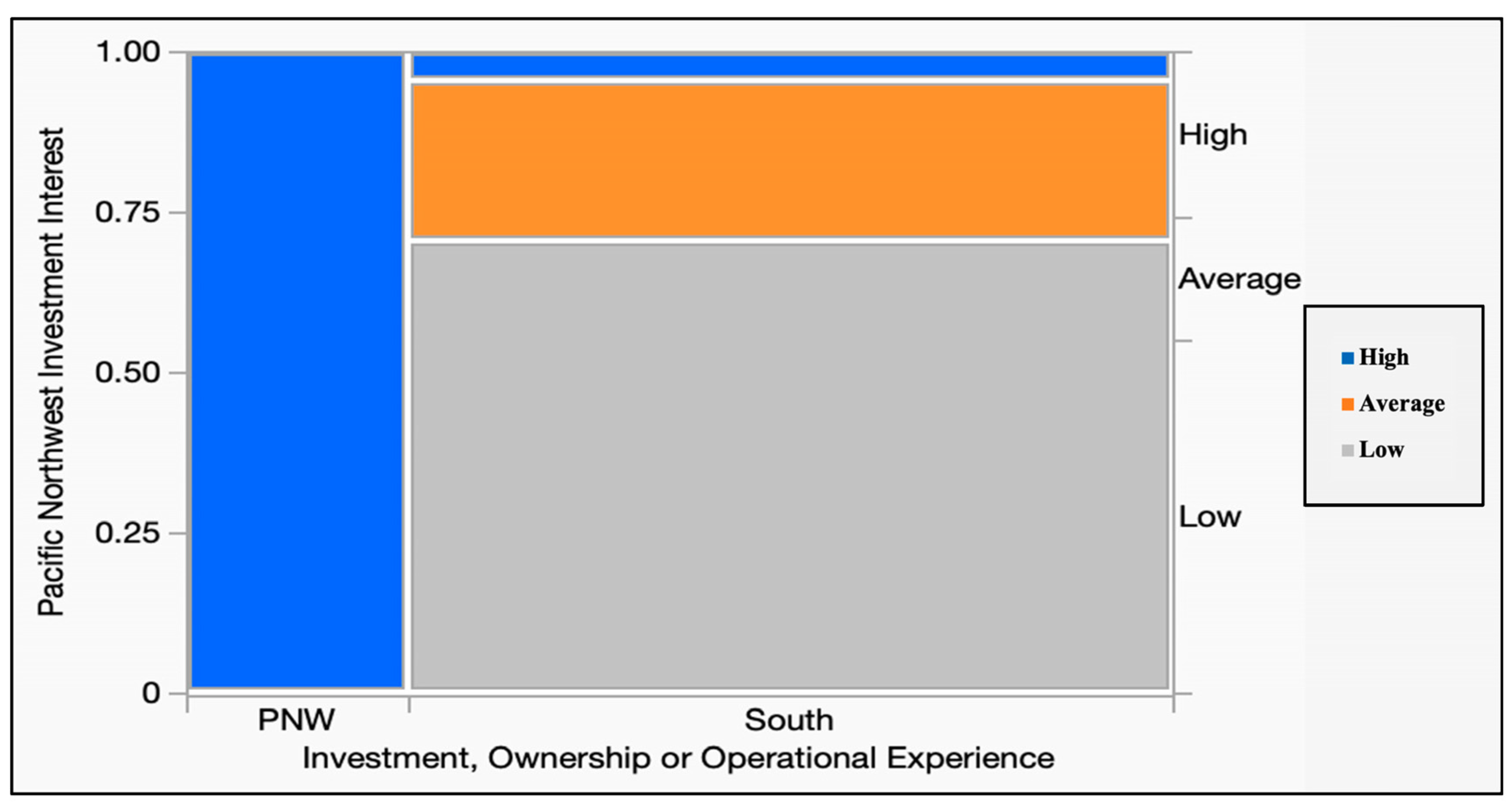
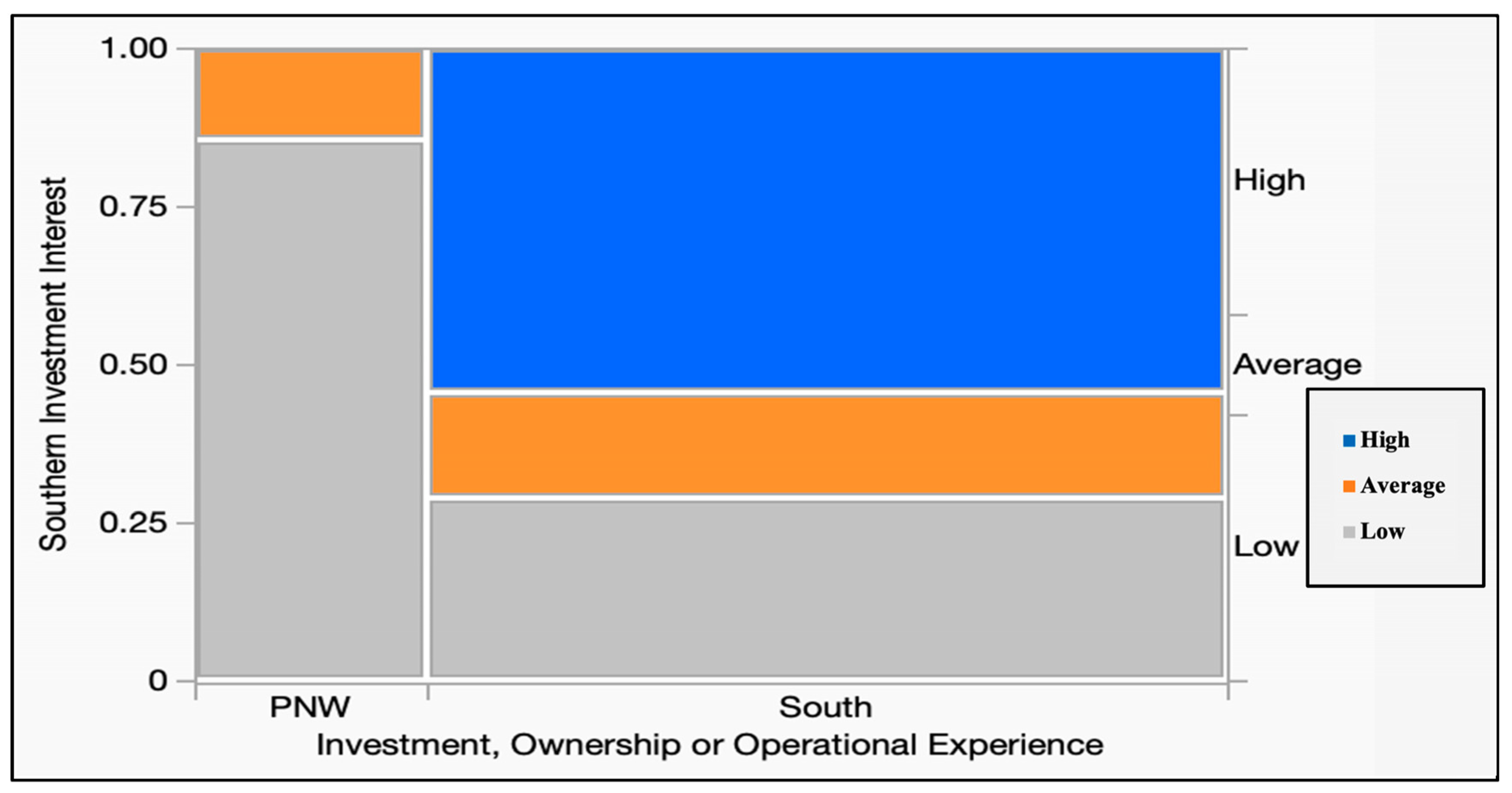
3.3. Hypotheses Testing Results

| Hypothesis | Response Variable | Explanatory Variable | Chi-Squared Test Statistic | Prob> ChiSq | Result |
|---|---|---|---|---|---|
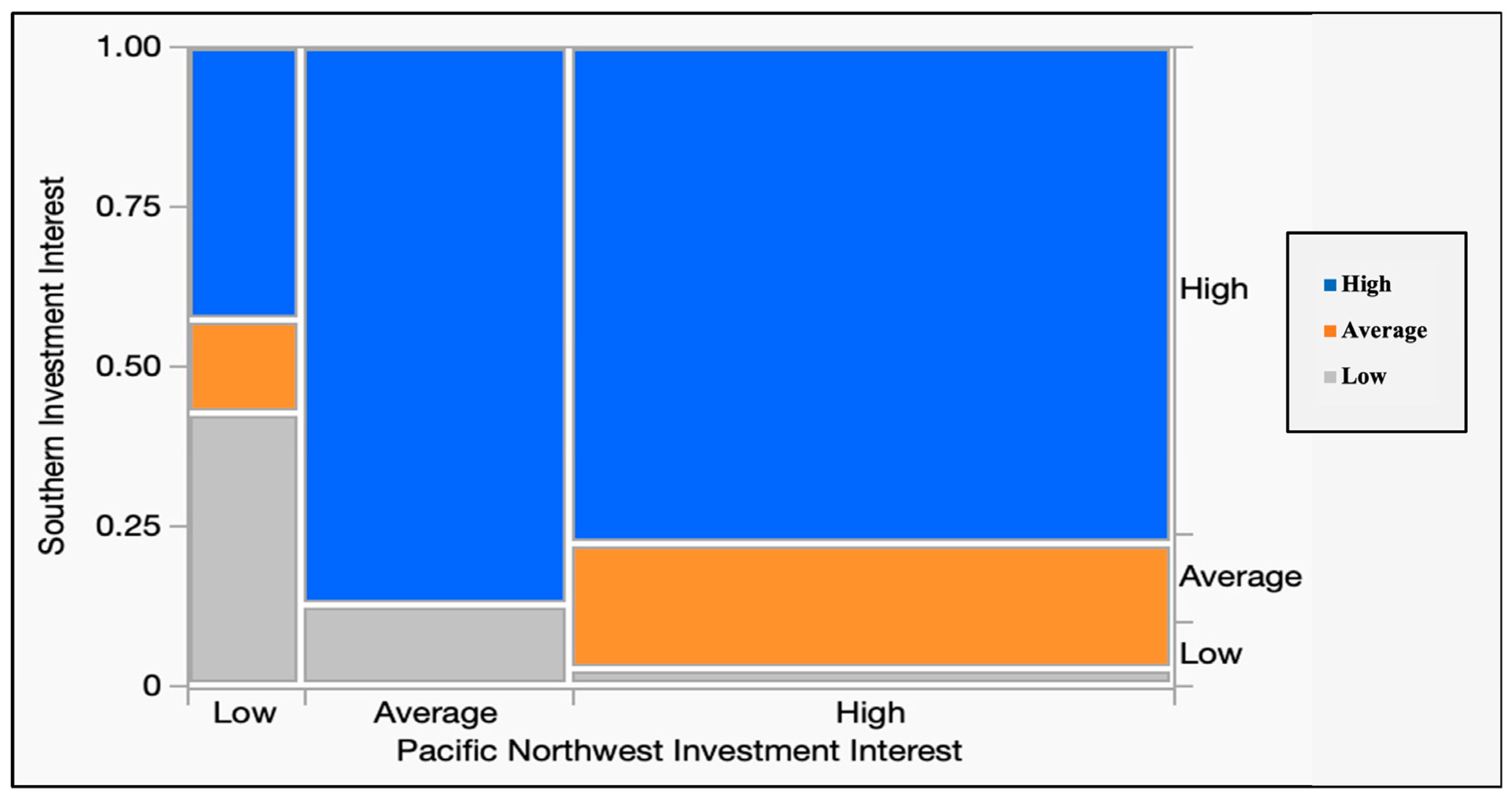
| H1: Investment interest in one region is not affected by investment interest in the other region. | PNW Investment Interest | U.S. South Investment Interest | 13.494 | 0.009 * | Reject H1 |
| U.S. South Investment Interest | PNW Investment Interest | 13.494 | 0.009 * | ||
| H2: Investment interest in one region is not affected by an investor’s existing ownership or investment experience in the same region. | PNW Investment Interest | Investment Ownership or Mgmt. in Either Region | 27.090 | <0.0001 * | Reject H2 |
| U.S. South Investment Interest | Investment Ownership or Mgmt. in Either Region | 10.169 | 0.006 * | ||
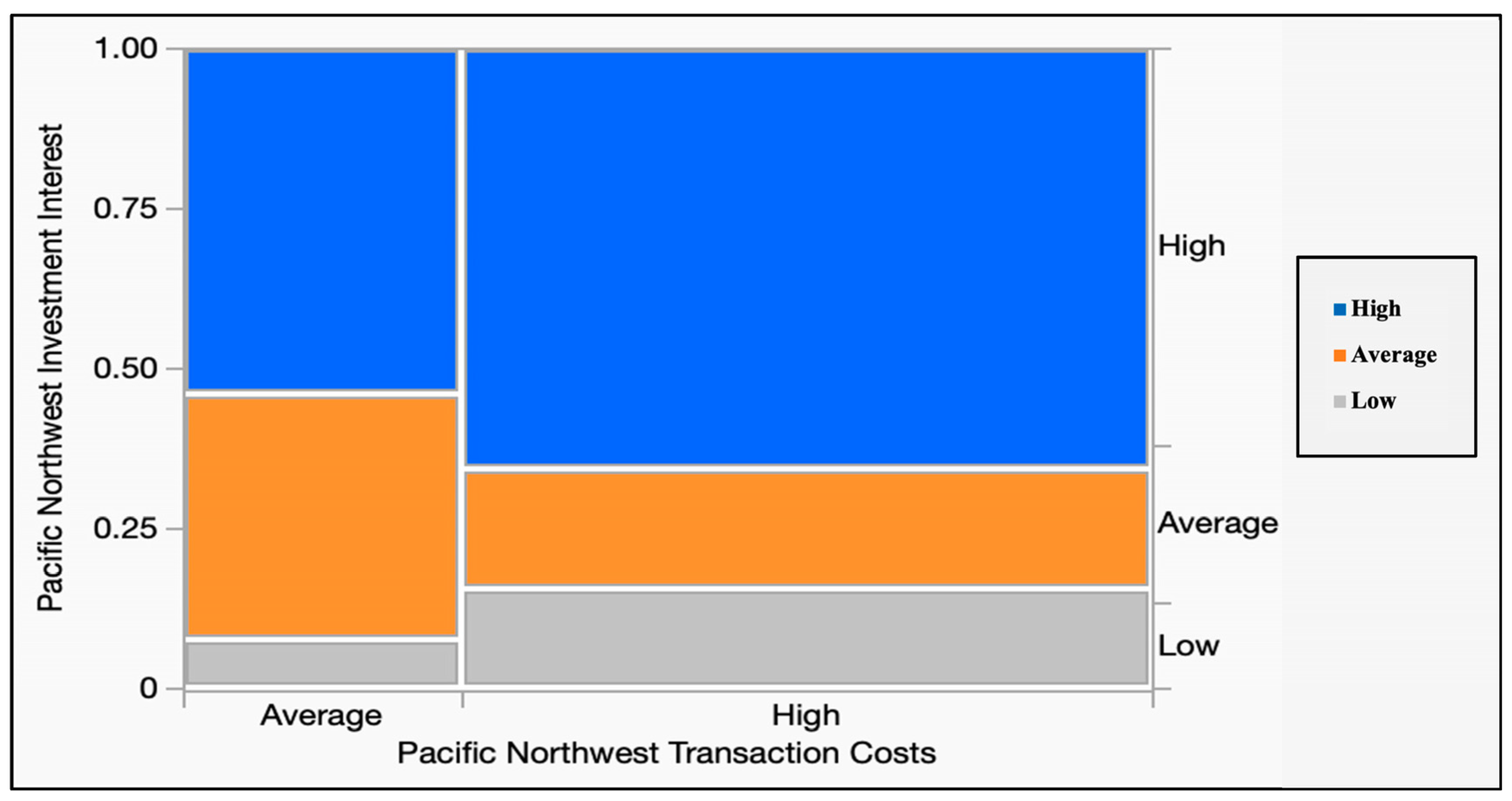
| H3: Investment interest in either region is not affected by the transaction costs incurred either in the same region or the other region. | PNW Investment Interest | PNW Transaction Costs | 0.806 | 0.6682 | Reject H3 |
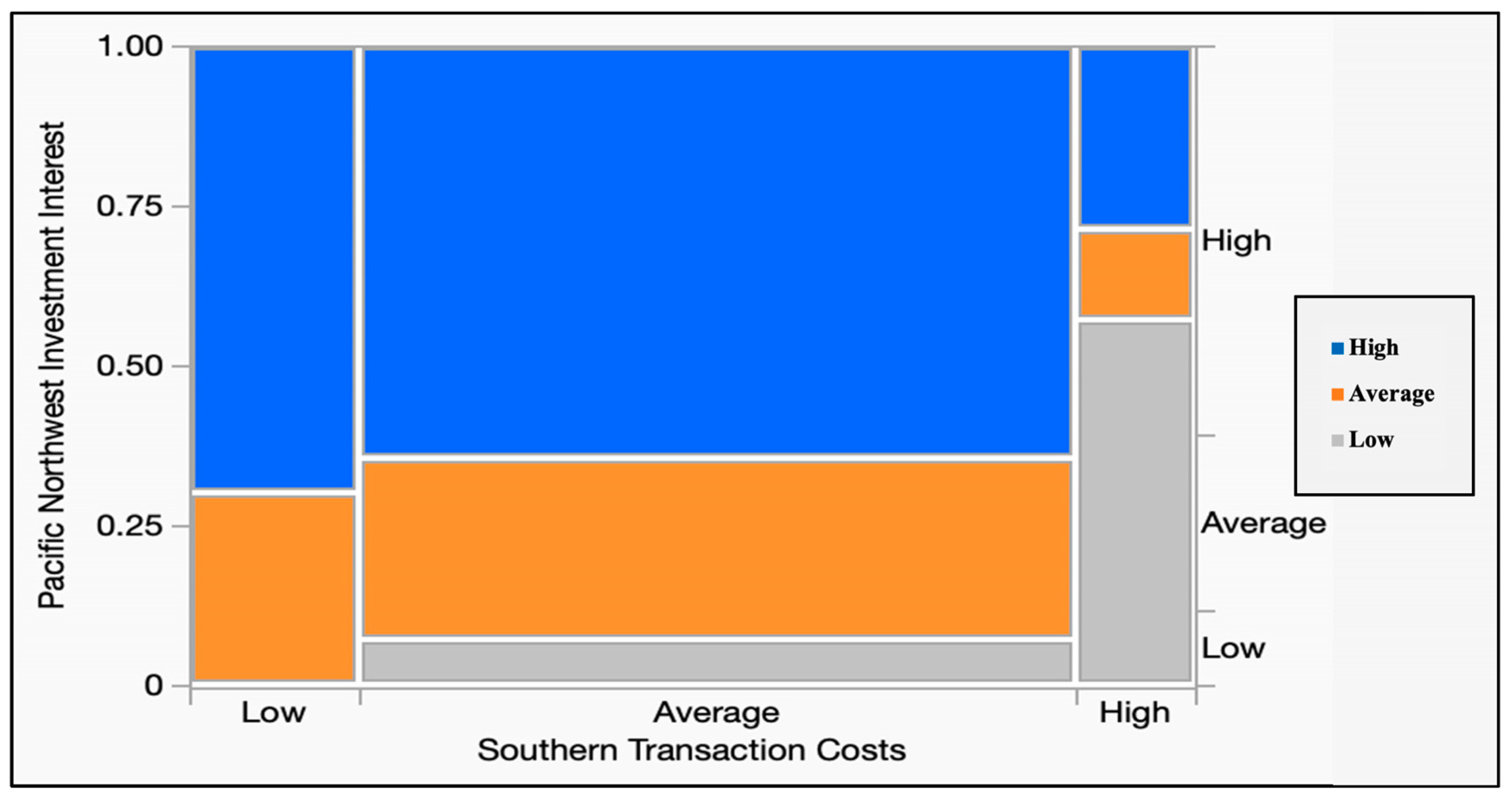
| PNW Investment Interest | U.S. South Transaction Costs | 11.814 | 0.018 * | ||
| U.S. South Investment Interest | PNW Transaction Costs | 3.245 | 0.1974 | ||
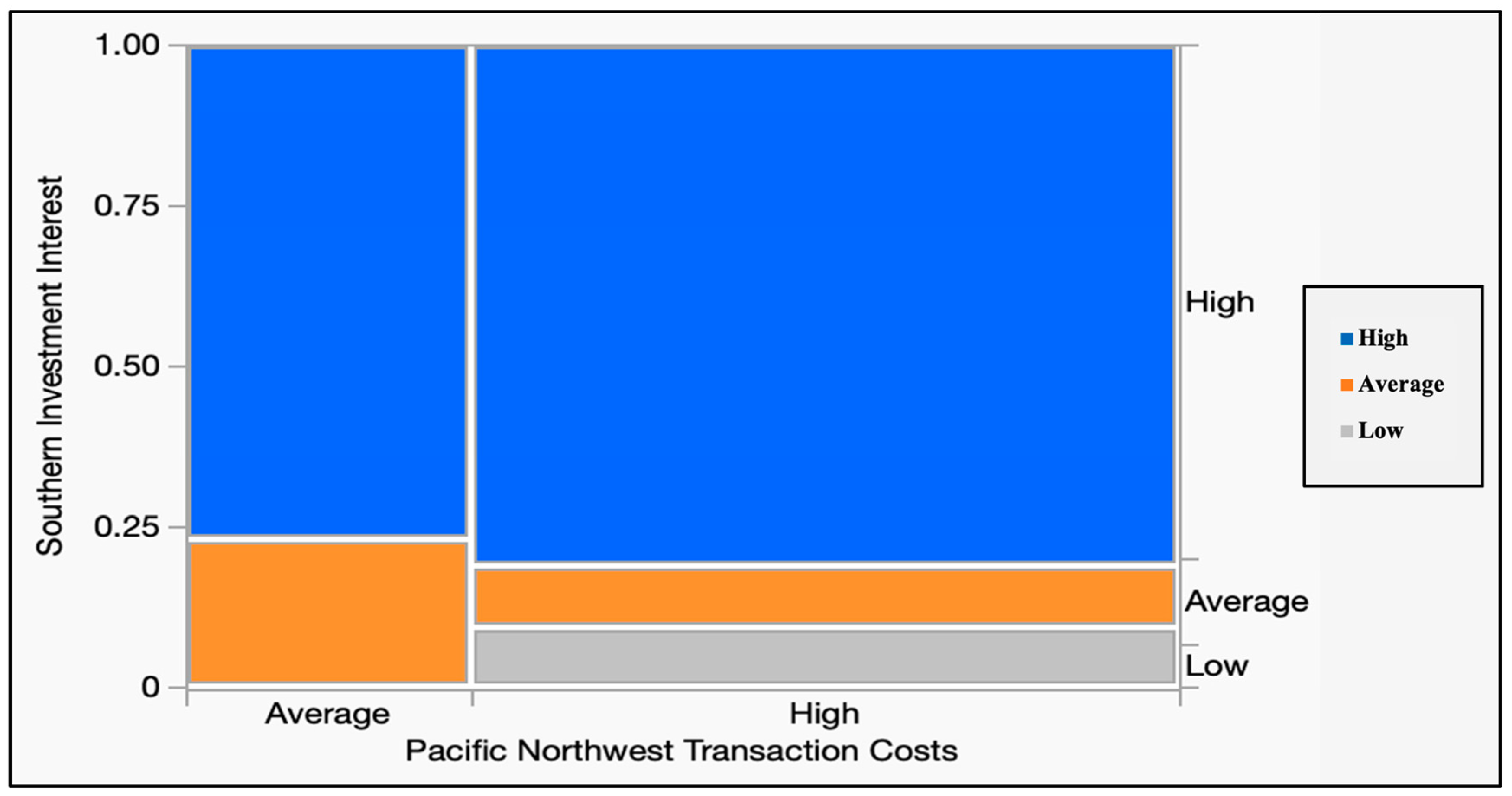
| U.S. South Investment Interest | U.S. South Transaction Costs | 10.037 | 0.039 * |


| Pacific Northwest Investment Interest | Total Responses | |||
|---|---|---|---|---|
| U.S. South Investment Interest | Low | Average | High | |
| High | 3 | 2 | 1 | 6 |
| Average | 1 | 0 | 7 | 8 |
| Low | 3 | 14 | 28 | 45 |
| Total | 7 | 16 | 36 | 59 |

| Pacific Northwest Investment Interest | Total Responses | |||
|---|---|---|---|---|
| Pacific Northwest Transaction Costs | Low | Average | High | |
| High | 6 | 11 | 26 | 43 |
| Average | 1 | 5 | 10 | 16 |
| Low | 0 | 0 | 0 | 0 |
| Total | 7 | 16 | 36 | 59 |

| Pacific Northwest Investment Interest | Total Responses | |||
|---|---|---|---|---|
| U.S. South Transaction Costs | Low | Average | High | |
| High | 4 | 1 | 2 | 7 |
| Average | 3 | 12 | 27 | 42 |
| Low | 0 | 3 | 7 | 10 |
| Total | 7 | 16 | 36 | 59 |

| U.S. South Investment Interest | Total Responses | |||
|---|---|---|---|---|
| Pacific Northwest Transaction Costs | Low | Average | High | |
| High | 0 | 3 | 10 | 13 |
| Average | 3 | 3 | 26 | 32 |
| Total | 3 | 6 | 36 | 45 |

| U.S. South Investment Interest | Total Responses | |||
|---|---|---|---|---|
| U.S. South Transaction Costs | Low | Average | High | |
| High | 3 | 1 | 3 | 7 |
| Average | 2 | 7 | 33 | 42 |
| Low | 1 | 0 | 9 | 10 |
| Total | 6 | 8 | 45 | 59 |

| Pacific Northwest Investment Interest | Total Responses | |||
|---|---|---|---|---|
| Investment, Ownership or Operational Experience in the Two Regions | Low | Average | High | |
| PNW | 0 | 0 | 7 | 7 |
| South | 17 | 6 | 1 | 24 |
| Total | 17 | 6 | 8 | 31 |

| U.S. South Investment Interest | Total Responses | |||
|---|---|---|---|---|
| Investment, Ownership or Operational Experience in the Two Regions | Low | Average | High | |
| PNW | 6 | 1 | 0 | 7 |
| South | 7 | 4 | 13 | 24 |
| Total | 13 | 5 | 13 | 31 |

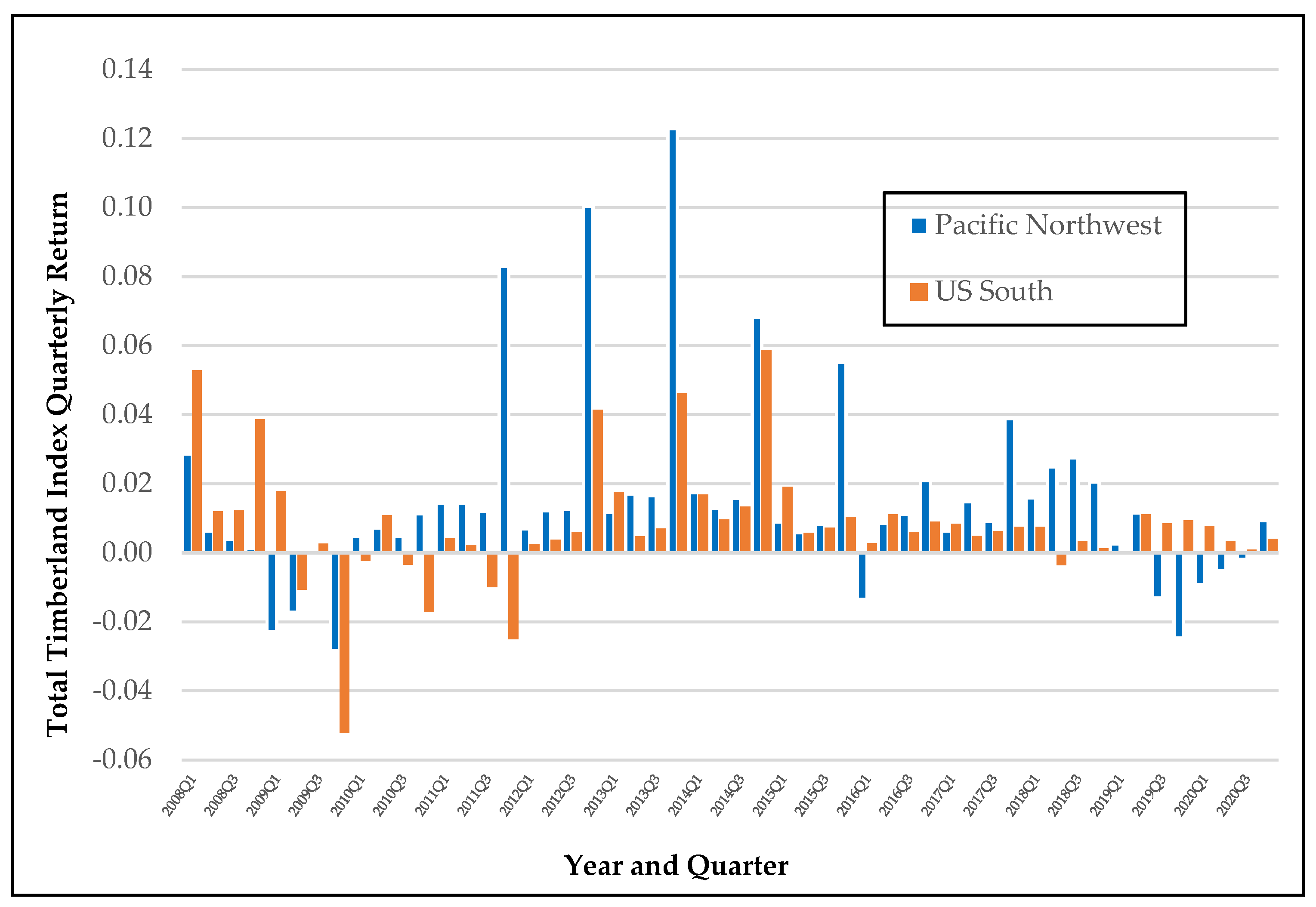
3.4. Regional Timberland Return Comparisons

| Timberland Region | Annualized Returns with Corresponding Standard Deviations (S.D.) | |||||
|---|---|---|---|---|---|---|
| 2016 until 2018 | 2015 until 2019 | 2014 until 2020 | ||||
| 3-Year | S.D. | 5-Year | S.D. | 7-Year | S.D. | |
| U.S. South | 2.16% | 1.24% | 2.75% | 1.15% | 3.61% | 3.07% |
| Pacific Northwest | 6.28% | 3.30% | 4.82% | 4.75% | 4.98% | 5.31% |
4. Conclusions
Author Contributions
Funding
Data Availability Statement
Acknowledgments
Conflicts of Interest
References
- Hardt, Ł. A history of transaction cost economics and its recent developments. Erasmus J. Phils. Econ. 2009, 2, 29–51. [Google Scholar] [CrossRef]
- Coase, R.H. The nature of the firm. Economica 1937, 4, 386–405. [Google Scholar] [CrossRef]
- Coase, R.H. The problem of social cost. J. Law Econ. 1960, 3, 1–44. [Google Scholar] [CrossRef]
- Hicks, J. A suggestion for simplifying the theory of money. Economica 1935, 2, 1–19. [Google Scholar] [CrossRef]
- Amihud, Y.; Mendelson, H. Transaction costs and asset management. In Global Asset Management: Strategies, Risks, Processes, and Technologies; Pinedo, M., Walter, I., Eds.; Palgrave Macmillan: London, UK, 2013; pp. 414–432. [Google Scholar]
- Allen, D.W.; Lueck, D. A transaction cost primer on farm organization. Can. J. Agric. Econ. 2000, 48, 643–652. [Google Scholar] [CrossRef]
- Mei, B. Timberland investments in the United States: A review and prospects. For. Pol. Econ. 2019, 109, 101998. [Google Scholar] [CrossRef]
- Evens, T. (TimberLink LLC., Johns Creek, GA, USA). Unpublished raw data. 2022. [Google Scholar]
- Hiegel, A.; Siry, J.; Bettinger, P.; Mei, B. Timberland transaction costs: Survey results and insights. J. For. Bus. Res. 2022, 1, 21–50. [Google Scholar]
- Chudy, R.P.; Cubbage, F.W. Research trends: Forest investments as a financial asset class. For. Policy Econ. 2020, 119, 102273. [Google Scholar] [CrossRef] [PubMed]
- Chambers, D.R.; Anson, M.J.P.; Black, K.H.; Kazemi, H.B. Alternative Investments: CAIA Level 1, 4th ed.; John Wiley & Sons, Inc.: Hoboken, NJ, USA, 2020; p. 928. [Google Scholar]
- The Land Report. 2022. Available online: https://landreport.com (accessed on 17 October 2022).
- Zhang, D.; Butler, B.J.; Nagubadi, R.V. Institutional timberland ownership in the US South: Magnitude, location, dynamics, and management. J. For. 2012, 110, 355–361. [Google Scholar] [CrossRef]
- Baral, S.; Mei, B. Development and performance of timber REITs in the United States: A review and some prospects. Can. J. For. Res. 2022, 47, 226–233. [Google Scholar] [CrossRef]
- Rayonier. 2022. Available online: www.rayonier.com (accessed on 5 August 2022).
- Forisk Consulting. 2022. Available online: https://forisk.com/resources/timber-reit-weekly-summary/ (accessed on 11 July 2022).
- Hoya Capital. 2022. Available online: https://www.hoyacapital.com/reit-sector/timber (accessed on 11 July 2022).
- Forest2Market. A New Report Details Regional Timberland Ownership and Class Profiles. 2019. Available online: www.forest2market.com (accessed on 3 November 2022).
- Kelly, E.C.; Crandall, M.S. State-level forestry policies across the US: Discourses reflecting the tension between private property rights and public trust resources. For. Pol. Econ. 2022, 141, 102757. [Google Scholar] [CrossRef]
- Rauscher, H.M.; Johnsen, K. Southern Forest Science: Past, Present, and Future, General Technical Report, SRS-75; Southern Research Station: Asheville, NC, USA, 2004; United States Forest Service. [Google Scholar]
- Talbert, C.; Marshall, D. Plantation productivity in the Douglas-fir region under intensive silvicultural practices: Results from research and operations. J. For. 2005, 103, 65–70. [Google Scholar]
- Binkley, C.S.; Aronow, M.E.; Washburn, C.L.; New, D. Global Perspectives on intensely managed plantations: Implications for the Pacific Northwest. J. For. 2005, 103, 61–64. [Google Scholar]
- Baldwin, S. Large US Timberland Transactions-Annual Summary (2015–2021); TimberMart-South: Athens, Greece, 2022; Unpublished raw database. [Google Scholar]
- Kessinger, J. (Forest2Market, Charlotte, NC, USA). Unpublished raw data. 2022. [Google Scholar]
- US Census Bureau, U.S. Department of Commerce. 2022. Available online: https://www.census.gov/construction/nrc/historical_data/index.html (accessed on 17 December 2022).
- Lee, H.Y. Goodness-of-fit tests for a proportional odds model. J. Korean Data Info. Sci. Soc. 2013, 24, 1465–1475. [Google Scholar] [CrossRef][Green Version]
- Heeringa, S.G.; West, B.T.; Berglund, P.A. Applied Survey Data Analysis, 2nd ed.; Chapman and Hall/CRC press: New York, NY, USA, 2017; 568p. [Google Scholar]
- Lyddan, C. (Fastmarkets RISI, Boston, MA, USA). Unpublished raw data. 2022. [Google Scholar]
- Mei, B. Investment returns of US commercial timberland: Insights into index construction methods and results. Can. J. For. Res. 2017, 47, 226–233. [Google Scholar] [CrossRef]
- Busby, G.; Binkley, C.S. Explaining the Disconnect between Lumber and Timber Prices. Nuveen Natural Capital Opinion Piece. 2021. Available online: https://documents.nuveen.com/Documents/Nuveen/Default.aspx?uniqueId=834a79b4-cbaf-4139-87ec-cf723a693f13 (accessed on 17 March 2023).


| Year | Pacific Northwest | Northeast | Midwest | South | U.S. Total |
|---|---|---|---|---|---|
| 2000 | - | - | - | 359,125 | 359,125 |
| 2001 | 133,263 | 10,724 | 36,826 | 2,353,289 | 2,534,103 |
| 2002 | 113,171 | 194,856 | 127,557 | 513,692 | 1,106,254 |
| 2003 | 179,476 | 509,257 | 166,043 | 991,668 | 1,954,377 |
| 2004 | 262,738 | 608,944 | - | 538,311 | 1,504,862 |
| 2005 | 628,667 | 332,612 | 653,690 | 972,670 | 3,009,322 |
| 2006 | 181,542 | 193,116 | 207,198 | 2,230,195 | 2,875,361 |
| 2007 | 510,895 | 78,914 | 70,820 | 1,265,681 | 2,157,773 |
| 2008 | 189,149 | 325,967 | 65,726 | 732,529 | 1,596,055 |
| 2009 | 96,494 | 141,718 | 23,876 | 290,135 | 653,120 |
| 2010 | 27,640 | 67,744 | 116,378 | 270,761 | 518,986 |
| 2011 | 124,193 | 473,370 | 68,878 | 260,263 | 987,033 |
| 2012 | 380,078 | 19,409 | 161,915 | 460,676 | 1,155,139 |
| 2013 | 366,798 | 38,727 | 2,015 | 515,257 | 983,720 |
| 2014 | 313,655 | 116,648 | 23,472 | 308,075 | 826,139 |
| 2015 | 287,584 | 63,281 | 48,967 | 540,810 | 1,022,716 |
| 2016 | 149,133 | 168,993 | 157,810 | 312,988 | 943,499 |
| 2017 | 108,012 | 9,308 | 37,644 | 199,389 | 431,934 |
| 2018 | 55,769 | 32,973 | 16,046 | 687,779 | 835,918 |
| 2019 | 24,015 | 184,610 | 283,323 | 257,774 | 1,094,232 |
| 2020 | 205,293 | 114,166 | 58,455 | 66,811 | 623,269 |
| 2021 | 316,366 | 102,645 | 101,118 | 360,060 | 973,748 |
| Totals | 4,653,933 | 3,787,983 | 2,427,757 | 14,487,939 | 28,146,686 |
Disclaimer/Publisher’s Note: The statements, opinions and data contained in all publications are solely those of the individual author(s) and contributor(s) and not of MDPI and/or the editor(s). MDPI and/or the editor(s) disclaim responsibility for any injury to people or property resulting from any ideas, methods, instructions or products referred to in the content. |
© 2023 by the authors. Licensee MDPI, Basel, Switzerland. This article is an open access article distributed under the terms and conditions of the Creative Commons Attribution (CC BY) license (https://creativecommons.org/licenses/by/4.0/).
Share and Cite
Hiegel, A.; Siry, J.; Mei, B.; Bettinger, P. Transaction Costs and Investment Interest in the U.S. South and the Pacific Northwest Timberland Regions. Forests 2023, 14, 1588. https://doi.org/10.3390/f14081588
Hiegel A, Siry J, Mei B, Bettinger P. Transaction Costs and Investment Interest in the U.S. South and the Pacific Northwest Timberland Regions. Forests. 2023; 14(8):1588. https://doi.org/10.3390/f14081588
Chicago/Turabian StyleHiegel, Andrew, Jacek Siry, Bin Mei, and Pete Bettinger. 2023. "Transaction Costs and Investment Interest in the U.S. South and the Pacific Northwest Timberland Regions" Forests 14, no. 8: 1588. https://doi.org/10.3390/f14081588
APA StyleHiegel, A., Siry, J., Mei, B., & Bettinger, P. (2023). Transaction Costs and Investment Interest in the U.S. South and the Pacific Northwest Timberland Regions. Forests, 14(8), 1588. https://doi.org/10.3390/f14081588