Article

Identifying the Minimum Number of Flood Events for Reasonable Flood Peak Prediction of Ungauged Forested Catchments in South Korea

Forest Restoration and Resources Management Division, National Institute of Forest Science, Seoul 02455, Republic of Korea
*
Author to whom correspondence should be addressed.
Forests 2023, 14(6), 1131; https://doi.org/10.3390/f14061131
Submission received: 31 March 2023 / Revised: 10 May 2023 / Accepted: 26 May 2023 / Published: 30 May 2023
(This article belongs to the Section Forest Hydrology)

Abstract

:
The severity and incidence of flash floods are increasing in forested regions, causing significant harm to residents and the environment. Consequently, accurate estimation of flood peaks is crucial. As conventional physically based prediction models reflect the traits of only a small number of areas, applying them in ungauged catchments is challenging. The interrelationship between catchment characteristics and flood features to estimate flood peaks in ungauged areas remains underexplored, and evaluation standards for the appropriate number of flood events to include during data collection to ensure effective flood peak prediction have not been established. Therefore, we developed a machine-learning predictive model for flood peaks in ungauged areas and determined the minimum number of flood events required for effective prediction. We employed rainfall-runoff data and catchment characteristics for estimating flood peaks. The applicability of the machine learning model for ungauged areas was confirmed by the high predictive performance. Even with the addition of rainfall-runoff data from ungauged areas, the predictive performance did not significantly improve when sufficient flood data were used as input data. This criterion could facilitate the determination of the minimum number of flood events for developing adequate flood peak predictive models.

1. Introduction

The frequency and severity of heavy rainfall events occurring in forested areas have escalated owing to increasing land use and rapid global climate change, with such events frequently resulting in flash flood disasters [1]. Flash floods cause considerable direct and indirect economic losses by damaging socioeconomic systems and infrastructure [2]. This trend is found worldwide, and damage to the environment is increasing as a result [3,4]. Moreover, susceptibility to flood-related threats is reaching dangerous levels [5,6]. Consequently, there is significant demand for researchers and governments to construct reliable and accurate flood prediction models and plan and implement sustainable flood risk management measures, with an emphasis on prevention and preparedness [7].
The development of statistical models and physically based distributed hydrological models (PB-DHMs) has traditionally been the focal point for simulating streamflow and flood peaks [8,9,10]. Statistical models utilize empirical datasets to determine underlying patterns for predicting future situations [11]. Common flood analysis models for flood prediction include multiple linear regression (MLR) [12], autoregressive moving average (ARMA) [13], and autoregressive integrated moving average (ARIMA) [14]. These are simple statistical models that predict floods quickly [15] and are easy to apply, which could be helpful in emergencies [16]. PB-DHMs take into consideration the physical features of a watershed, such as topography, soil characteristics, vegetation cover, and climate, when predicting the behavior of the hydrological system. The advantage of these models is their ability to account for geographic heterogeneity within a watershed and the significant knowledge of the hydrologic system [17,18].
The two approaches, statistical models and PB-DHMs, however, have disadvantages in flood prediction. Statistical models cannot explain variance in catchment sizes owing to their lack of mechanistic understanding [11]. Furthermore, they are dependent on historical datasets and generally require several datasets for capturing seasonal patterns and producing reliable long-term predictions. Therefore, statistical models may not be appropriate for predicting floods in areas with limited or incomplete datasets [19]. The PB-DHMs require rigorous calibration to produce correct predictions. This process is often time consuming, difficult, and requires abundant data and high levels of expertise for operation [20,21]. Moreover, these models require substantial computational resources and high-resolution geographical data pertaining to catchment characteristics, as well as the initial boundary conditions [22]. Therefore, despite extensive research, an optimal model remains elusive, and it remains difficult to accurately predict a flood peak, particularly in forested catchments with complex topological features.
Machine learning approaches have recently emerged as promising technologies that could partly solve some of the aforementioned problems. This is because machine learning structures, which include a significant number of parameters, are complex and can effectively explain the relationships of non-linear variables. Therefore, complicated mathematical formulations of the physical processes of flooding can be mimicked by machine learning [23]. Several researchers have found that predictive models based on machine learning generally have superior prediction performances [24] and are particularly effective for predicting flooding events [23,24,25]. Consequently, the field of flood prediction has moved toward data-driven techniques.
Flood prediction in ungauged areas remains challenging and relevant research on this topic is scarce. A few models that could potentially accurately predict flood peaks have been investigated, particularly for ungauged catchments. A particular concern is that flood hazards are increasing in severity and frequency. However, almost all the areas remain unmeasured, placing a significant limitation on conventional approaches such as statistical models or PB-DHMs. Thus, these limitations have resulted in the development of machine learning-based data-driven models. When a hydrological model is calibrated to a single unique catchment, the developed model provides the most accurate simulation results [26]. Furthermore, data-driven approaches could benefit from a vast cross-section of heterogeneous training data, as knowledge could be transferred between different catchments [27]. This implies that floods from various catchments could be studied through one predictive model based on machine learning. Few studies, however, have investigated flood peak prediction for ungauged areas by considering the differences in the characteristics of the basin and the interrelationships with flood characteristics. Moreover, few studies have collected sufficient data to develop optimal predictive models.
Deep learning approaches are data-driven models; therefore, the predictive accuracy is determined by the quality and quantity of the input data [28]. Thus, to develop a reasonable predictive model, an adequate amount of data must be collected, and the model should be trained based on these data. In addition, to develop a region-specific flood peak predictive model, plans must be established for collecting flood data in each region. However, studies presenting the minimum amount of flood event data required for the accurate prediction of flood peaks and establishing assessment standards for data collection remain scarce.
Therefore, the current study aims to (1) identify whether a machine learning model is suitable for predicting a flood peak in ungauged areas (only for the prediction of a flood peak, which is the maximum streamflow of a singular rainfall-runoff event) and (2) present the data of the minimum number of flood events required to effectively predict flood peaks.

2. Materials and Methods

2.1. Study Areas

The rainfall and flow data required for developing a flood prediction model were collected from 40 forest sites managed by the National Institute of Forest Science, Seoul, South Korea (Figure 1). The data from each catchment were collected over a minimum of 1 year and a maximum of 39 years. The size of the catchment areas ranged between 2 ha and 969 ha, and most were small forested catchments below 100 ha. The slopes of the 40 catchments varied, with the average slope being 20.0–4.9 degrees. Various basin characteristics were reflected on the forest floor, including broadleaf, coniferous, and mixed forests (Table S1).
A water level gauge dam was installed at each site that included a 90° or 120° V-shaped notch or square notch, and the flow data were collected every hour through a pressure-type water level gauge or float-type water level meter. A rain gauge was also installed at each site to collect rainfall data every 10 min.

2.2. Identifying Flood Peaks

We identified the flood events and extracted information from the observed streamflow. Every peak in the streamflow data was isolated and considered a potential flood event. The 95th percentile streamflow value was calculated for each catchment, and this value was designated as the threshold for a flood peak, i.e., when an observed streamflow was higher than the threshold, it was considered a flood event.
Although such streamflow represents a substantial flow, not all events inundating the embankment were considered flood events. However, if all these data were used, the machine learning model could be trained with substantially more data, which could facilitate more reasonable predictions of extreme streamflow. The eventual result would be an effective predictive model for the highest streamflow status and may be highly correlated with flood events [10].
Another subjective criterion was used for the identification of flood events. We considered a flood event to have ended if no rainfall occurred for 3 consecutive days following the end of precipitation. This criterion was added because most of the streamflow was dominated by baseflow after 3 days with no rainfall, particularly in small forested catchments [29]. As the effects of torrential rainfall usually dissipate after 3 days, this threshold was used to identify the end of a flood event.

2.3. Flood Predictive Model

2.3.1. Random Forest

The random forest (RF) model, a popular machine learning algorithm, is an ensemble learning technique that integrates the results of numerous decision trees to produce a single final prediction [30]. As the ensemble of decision trees minimizes the variance of the predictions and prevents overfitting to noisy data, the RF model is less affected by noise and outliers compared with the other approaches [31]. Moreover, this model is renowned for its accuracy in prediction tasks despite its simplicity and has a wide range of applications.
Long short-term memory (LSTM) has recently been used as a deep learning approach to predict time-series data; therefore, we adopted the RF model in our study. The parameters of LSTM are updated continuously according to the time series. The rainfall-runoff model is a suitable structure for time-varying processes in nature where values depend on their own previous values. By contrast, the model we developed for this study was based on independent flood peaks for the purpose of understanding the unique characteristics of floor peaks; therefore, we used the RF model. Three RF model hyperparameters, namely, n_estimation, max_depth, and max_features, were tuned for optimization.

2.3.2. Streamflow and Meteorological Dataset

Streamflow and meteorological datasets, including rainfall and potential evapotranspiration (PET) data, were used as the dynamic variables for predicting flood peaks. The Korea Meteorological Administration (KMA), Seoul, South Korea, offers extremely short-term rainfall predictions up to a maximum of 6 h; therefore, we used hourly data in the current study. The streamflow and rainfall data are in situ measurements collected from water level gauge dams in 40 forested catchments. To eliminate the impact of streamflow derived from the different catchment sizes, we standardized all streamflow and rainfall data units to millimeters. The PET data were calculated based on a meteorological dataset collected by the Automated Synoptic Observation System currently operated by the KMA. The PET was determined based on the daily evapotranspiration estimation equation provided by the UN Food and Agriculture Organization (FAO) [32]. The PET estimation equation is as follows:
P E T = 0.408 R n G + γ 900 / T + 273 u 2 ( e s e a ) + γ ( 1 + 0.34 u 2 )
where R n is net radiation (MJ m−2 day−1), G is the soil heat flux density (MJ m−2 day−1) that can be ignored for daily calculations, T is the air temperature at 2 m height (°C), u 2 is the average wind speed at 2 m height (m s−1), e s is the vapor pressure of the air (kPa), e a is the actual vapor pressure (kPa), is the slope of the vapor pressure curve (kPa °C−1), and γ is the psychrometric constant (kPa °C−1). Allen et al. [32] suggested a comprehensive set of equations for computing all the parameters of Equation (1) in accordance with the available meteorological data and a time-step computation. In this study, we ignored G for estimating the daily PET. The sine method, which assumes that latent flux follows a sine curve throughout a day, was used to estimate the hourly PET from the daily values [33].

2.3.3. Catchment Characteristic Variables

Six catchment characteristics were used to reflect the characteristics of different catchments, which are the catchment area, mean slope, stream slope, stream length, mean soil depth, and hypsometric (Table S1). The catchment area at the point where the flow gauge dam is located was calculated for the catchment area, and the average slope of the catchment area was determined as the mean slope. For the stream slope, the difference between the maximum and minimum heights was divided by the stream length [34]. For average soil depth, we used the Forest Site and Soil Map provided by the Korea Forest Service [35], Daejeon, South Korea, and the Hypsometric Integral Toolbox of ArcGIS (Esri, Redlands, CA, USA) for the hypsometric [36]. It is worth noting that these are static variables that all have the same value for the catchment characteristics of each catchment, unlike the streamflow and meteorological data that vary for each flood event.
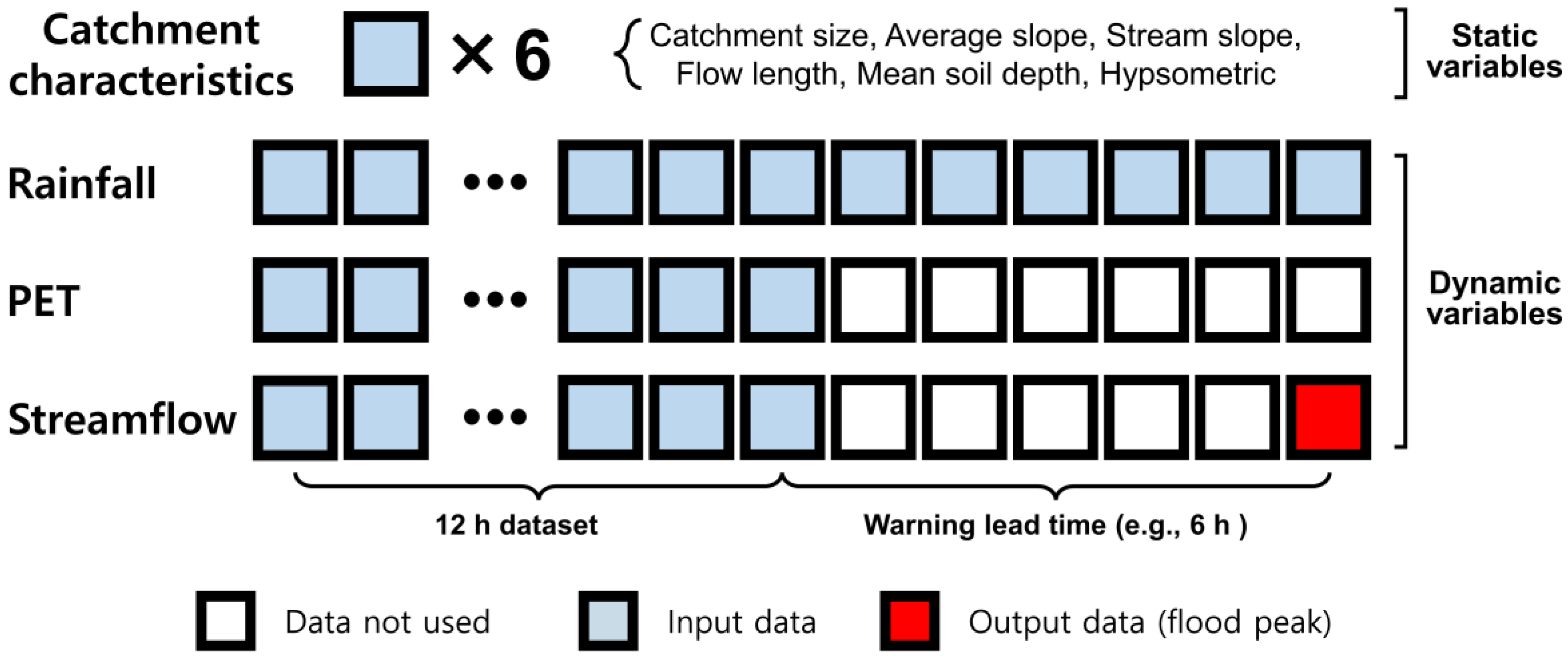
Figure 2 shows the input and output variables used in this study. The rainfall, PET, and streamflow data of the previous 12 h were used to predict the flood peak, and rainfall data up until the flood peak were used. Furthermore, to understand the differences between the catchments, the data on six catchment characteristics were included in the input datasets. As the KMA provides extremely short-term rainfall prediction up to 6 h from the current period, the warning lead times for setting the flood peak alarm were set at 1 h and 6 h.

2.4. Performance Evaluation

The root mean square error (RMSE) and Nash–Sutcliffe efficiency (NS) were used to evaluate the performances of the predictive models.
R M S E = 1 N i = 1 N P i P i ^ 2
N S = 1 i = 1 N P i P i ^ 2 i = 1 N P i P ¯ 2
where P i is the observed flood peak at time i (mm), P i ^ is the predicted flood peak at time i (mm), P ¯ is the average value of observed flood peaks (mm), and N is the total number of observed flood peaks. The RMSE is a commonly used metric for comparing the values predicted by a model with the values actually observed [37]. This value can show the predictive errors, with a lower RMSE value denoting superior prediction. The NS value equals 1 when the model is perfect, and the estimation error variance is equal to zero [38,39]. However, if the observed mean is a better predictor than the model, it could be less than zero. Therefore, RMSE and NS values that are close to 0 and 1, respectively, are considered accurate for flood prediction models.

3. Results and Discussion

3.1. Prediction of Flood Peaks in Ungauged Areas

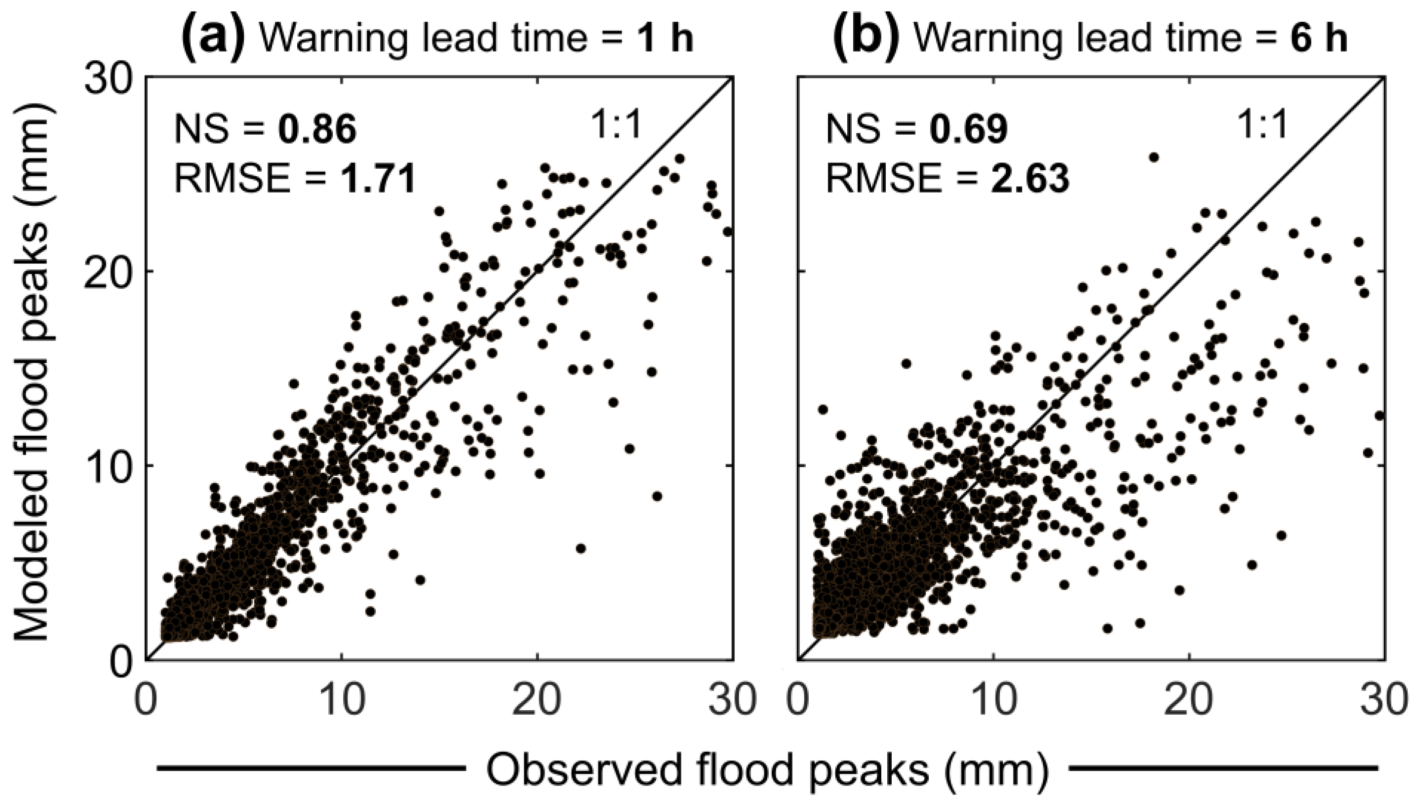
We conducted analyses of the relationship between the observed and the modeled flood peaks to determine whether the machine learning approach was suitable for predicting flood peaks in ungauged catchments (Figure 3). In the prediction model, one out of 40 catchments was assumed to be an ungauged catchment, and the flood data from the remaining 39 catchments were used for model development. The flood peak of the hypothesized ungauged area was predicted based on the developed model. Additionally, to holistically identify the prediction rate from all the catchments, all 40 catchments were assumed ungauged in order; thus, 40 different prediction models were developed. After model development, the prediction performances of the shortest warning lead time (1 h) and the longest warning lead time (6 h) were compared. In Figure 3a, a higher performance is shown for the flood peak prediction with 1 h warning lead time. When the warning lead time was 1 h, the NS value was 0.86 and RMSE 1.71, i.e., the predictive accuracy was high. By contrast, with a warning lead time of 6 h, the NS value was 0.69 and the RMSE 2.63, indicating that the predictive performance declined as the warning lead time increased.
Considering the extreme difficulty of predicting the flood peak of ungauged areas [40], our prediction results showed high accuracy for both cases (1 h and 6 h warning lead time). Moreover, we determined that the RF model could be used effectively to predict the flood peak of an ungauged catchment.
As shown in Figure 3, several events with higher flood peaks were identified in the observed flood peaks compared with the predicted flood peaks for relatively substantial flooding. Therefore, some flood peak events appear to have been underestimated. Underestimation could trigger false alarms, as the actual flooding amount could exceed the predicted flooding amount, and the risk would be higher when an actual warning system is operated [41]. Such underestimation mostly occurred when flooding during the summer rainy season was predicted. In South Korea, the four seasons are distinct, and the rainy season occurs between June and July because of a combination of high-pressure systems [42]. As significant preceding rainfall could occur during the rainy season, the soil near the catchment could be close to saturation, and these circumstances could generate significant flooding, even with relatively low rainfall events [1].
If more input variables related to flooding, such as the antecedent precipitation index (API) that quantify the rainfall status, were added, the model could be strengthened, and flood peak prediction could be accurate. In addition, in the future, if the machine learning model specialized for prediction accuracy and the physical model that physically describes the preceding rainfall and soil saturation could be combined, a deeper understanding of heavy rainfall linked to soil saturation could be attained. Moreover, flooding amounts could probably be predicted with higher accuracy.

3.2. Predictive Performance Changes with Data Accumulation

Analysis was conducted to determine the minimum number of flood events required for effective flood peak estimation. As the machine learning model is a data-driven model and is directly affected by the quality and quantity of data [28], we compared the relationship between data quantity and prediction capacity. The number of flood events contained in the data of the training dataset was increased gradually to observe any changes in prediction accuracy (Figure 4). Note that only the warning lead time of 1 h was considered in the comparison of the prediction performance, as the lag time of the forest catchment did not generally exceed 2 h [43]. Additionally, a warning lead time of 1 h is considered the most important for a flash flood warning system for mountain village inhabitants.
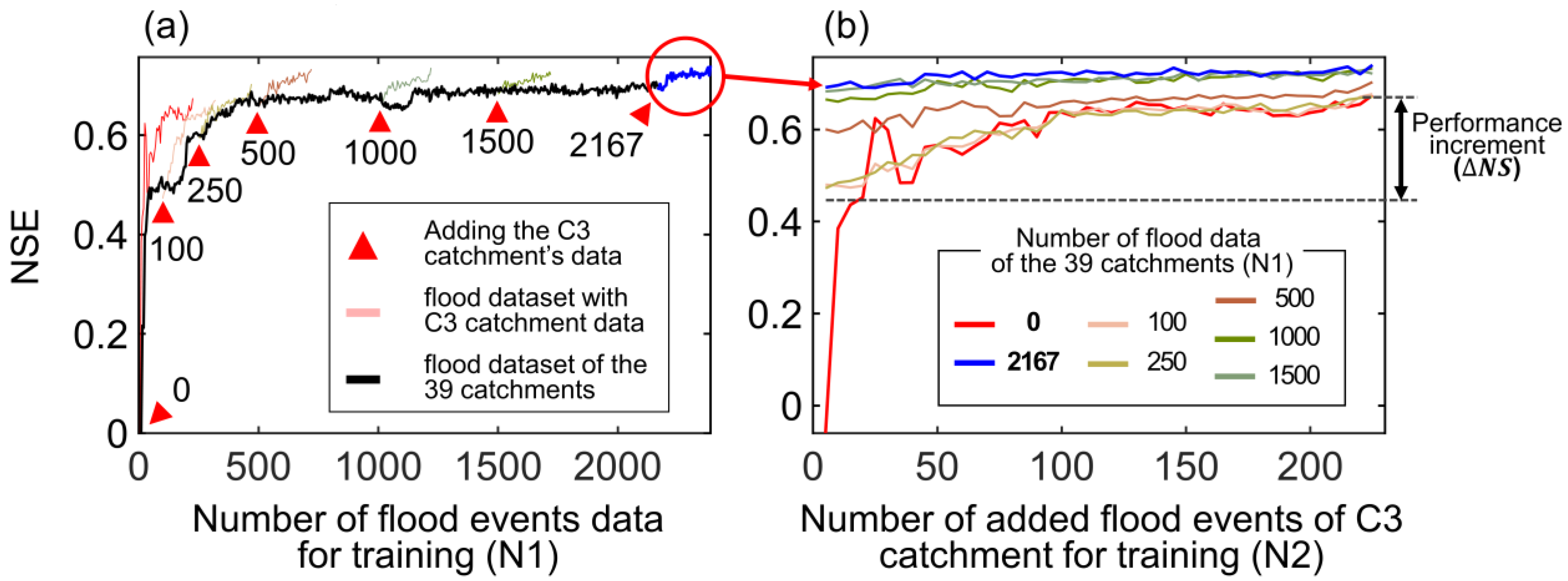
A site (catchment C3; Table S1) with numerous flooding events was selected as the hypothesized ungauged area. In order to generate a training dataset, five flood events were selected randomly and repeatedly added to the collected flood data from the remaining 39 catchments until all flood events were included (first loop in Figure 4). The test dataset was constituted by arbitrarily selecting 30% of the flood dataset of site C3. Each time the number of flood events (N1) changed, the predictive model was developed, and the predictive accuracy was determined by comparing the predicted values with the test dataset (Figure 5). Figure 5a shows the relationship between the number of flood events (training dataset) and the predictive performance. The number of flood events for developing machine learning could be identified, which showed higher flood peak prediction performance in the ungauged catchment as the training dataset increased.
We determined whether the flood peak data of ungauged catchments were sufficiently predictable by each prediction model with a different number of flood events. We repeatedly added the flood peak dataset of the C3 site (hypothesized ungauged catchment) to the training dataset used in the existing predictive model to identify changes in prediction performance (Figure 5b). The analysis was performed to determine the extent of changes in the prediction performance when the flood data of the ungauged catchment were added to the flood dataset used to develop the prediction model; 0, 100, 250, 500, 1000, 1500, and 2167 flood events that were selected arbitrarily from the flood peak dataset of 39 catchments were added to the flood peak data of the C3 catchment. Subsequently, the predictive accuracy was estimated (second loop in Figure 4). Seventy percent of flood events in site C3 were selected, and five flood events were repeatedly added each time to merge with the existing data. Therefore, even when all the data were merged, there were no flood events overlapping with the test datasets.
A predictive model was developed using the merged dataset, and its predictive accuracy was estimated. As the data from site C3 were added, the predictive accuracy increased (Figure 5b). However, the increase in performance accuracy differed significantly according to the number of flood events included in the data of the 39 catchments. We defined the increased performance accuracy as the performance increment ( N S ) after all the data from the hypothesized ungauged catchment (site C3) had been added. The calculation equation is as follows:
N S = N S f l o o d s N S 0
where N S 0 is the NS value of the predictive model before adding the flood events of the hypothesized ungauged catchment, and N S f l o o d s is the NS value after adding all the flood events of this catchment. Therefore, N S is the difference in performance accuracy before and after adding all the flood events of the ungauged catchment.
For zero flood events, the N S value was the greatest (red line in Figure 5b), and for 2167 flood events, the N S value was the lowest (blue line in Figure 5b). As shown, the N S value gradually declined as the number of flood events included in the data of the 39 catchments increased. A small N S value implied that despite collecting continuous flood data from an ungauged catchment, only a slight improvement was observed in the performance. Thus, even if sufficient flood data were obtained, the predictive performance would hardly improve with flood data from ungauged catchments being added continuously. This implies that despite adding significant flood data from ungauged catchments—in this case, 70% of flood data for 39 years—if the predictive accuracy does not increase, the training set used to develop the existing model probably already sufficiently describes the characteristics of the ungauged catchment. Therefore, with a sufficiently small N S , an adequate number of flood events were contained in the data for predicting the flood peaks in ungauged catchments. For the same reason, this process could be considered standard for a minimum number of flood events to be included in the data for predicting flood peaks in ungauged catchments.

3.3. Minimum Number of Flood Events in Data Collection

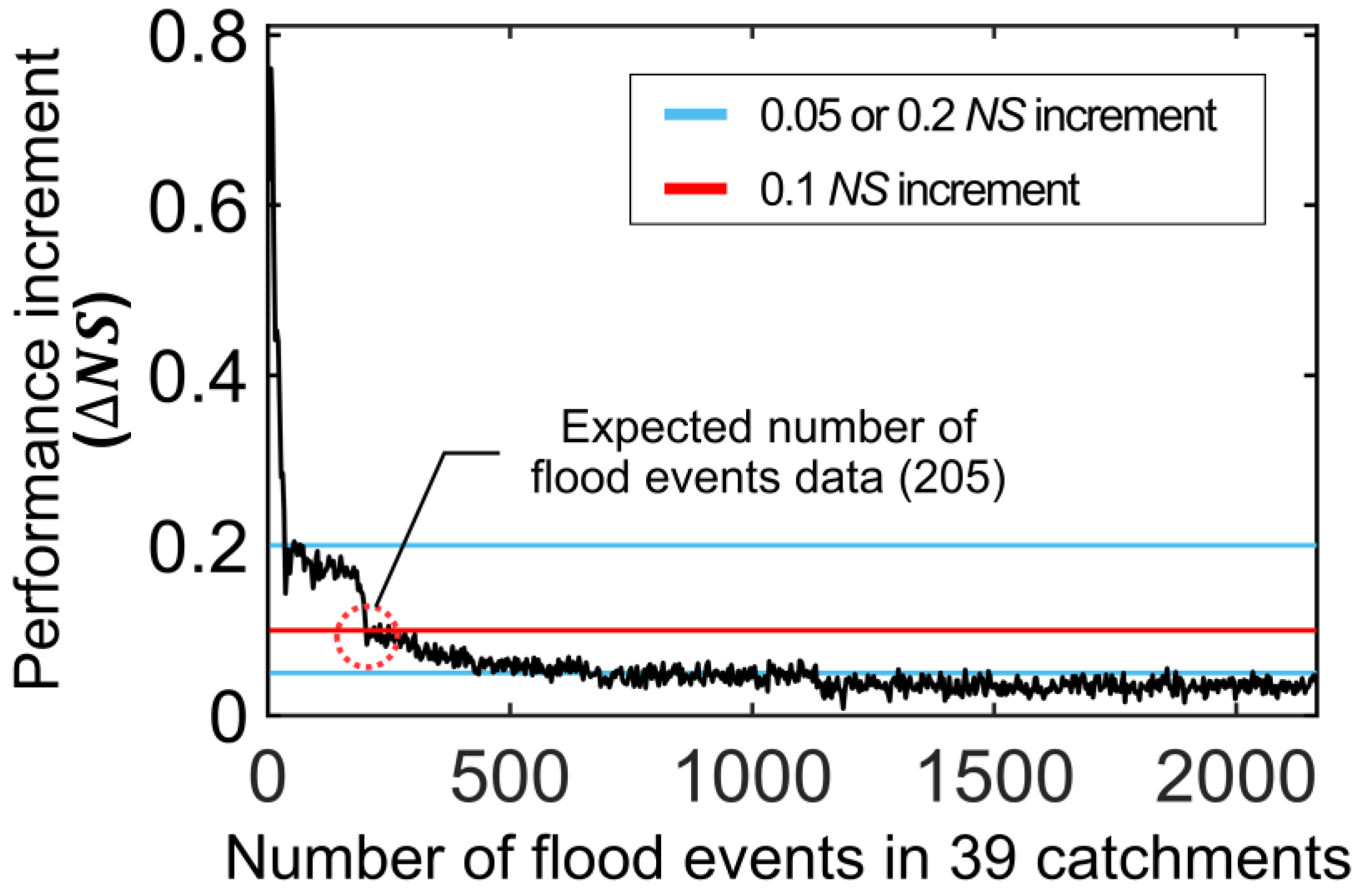
To present the minimum number of flood events in the collected data and effectively predict the flood peak in ungauged catchments, we analyzed the number of flood events in the data collected from 39 catchments as well as the relationship with N S (Figure 6). As the number of flood events in 39 catchments increased, N S decreased. When we set N S at 0.1 as a criterion for the minimum amount of data required, we considered data with 205 flood events as the expected number of flood data collection. This is ascribed to the predictive model being developed based on a set of 205 arbitrarily selected flood events, and even when a large number of flood events from site C3 were added, the N S value only increased below 0.1. The predictive performance did not significantly increase even when data from site C3 was added; therefore, data for 205 flood events could be considered to adequately reflect the flood peak characteristics of site C3. Note that these calculations are based on a subjective standardization of N S ; therefore, depending on the accuracy goal of a predictive model, different standards could be applied, such as 0.05 or 0.2 (blue lines in Figure 6). In this study, N S of 0.1 was set as the standard for collecting the minimum number of flood events.
However, the data for 205 floods were derived from a case study. Only site C3 was assumed to be an ungauged catchment, and flood data were extracted randomly from the 39 catchments. Therefore, it is difficult to present the above conclusions as a general minimum amount of data for predicting the flood peak in ungauged forest catchments in South Korea. In order to manage this problem, seven different catchments were selected, and random sampling was repeated multiple times, which involved adding flood events (third loop in Figure 4). In order to determine the required number of flood events, a sufficient amount of flood data from hypothesized ungauged areas must be added and compared. Therefore, seven catchments, with at least 100 flood events recorded over a period of 10 years or longer, were selected (bold catchments in Table S1). For generalization, random sampling was performed 1000 times for each catchment, and the minimum number of flood events was determined for each iteration to derive a total of 7000 result values (Figure 7). The median of the distribution was 75, the mean value was 94, and the standard deviation was 76.6. The 90th percentile of this distribution was 195 flood events, and the 95th percentile was 240 flood events. Therefore, when 195 and 205 flood events were gathered, the flood peaks of ungauged forest catchments could be estimated effectively at 90% and 95% probability, respectively. Additionally, this distribution could be used to establish a data collection strategy for a flood peak prediction model of ungauged catchments or for flood warning services.
Region-specific models must be developed for the effective prediction of floods in ungauged catchments, as flood characteristics in each region vary with different climate and environmental characteristics. Rasheed et al. [10] found that flood prediction in 18 distinct hydroclimatic regions in the United States showed significant regional dependence. Kratzert et al. [27] developed a rainfall-runoff model using LSTMs, which is a data-driven approach. These authors found that the embedding layer showing the characteristics of the predictive model exhibited regional dependency despite excluding longitude and latitude data during the model development process. Consequently, individual models must be developed for each region to facilitate a more accurate prediction of floods.
Therefore, the method presented in this study could be employed in the future for establishing a strategy for region-specific flood peak predictive model development to enable effective flood estimation of ungauged catchments. The study results could be particularly useful for establishing plans for estimating floods in forest watersheds. Forest catchments are often subject to significant environmental restrictions and have limited accessibility; therefore, data collection is quite difficult in forest catchments. Developing a model for more accurate forest watershed flood prediction in South Korea requires a strategic approach to the collection of flood data. In the future, establishing data collection strategies based on these methods could facilitate a more economical and time-efficient approach to model development.

4. Conclusions

A machine learning model based on RF information was developed to predict flood peaks in ungauged catchments using data from 40 small forested catchments. Six static variables for catchment characteristics and three hourly dynamic variables for meteorological features were used as training datasets to develop the predictive model. The predictive performance was evaluated using the RMSE and Nash–Sutcliffe efficiency, and high predictive performance was obtained for two warning lead times, namely, 1 h and 6 h. High predictive accuracy demonstrated the applicability of machine learning for estimating flood peaks in ungauged areas. This study confirmed a non-linear relationship between the number of flood events contained in the data for training datasets and the predictive accuracy. Based on this relationship, we found that the predictive accuracy did not increase significantly when a sufficient number of floods were included in the model development process; however, additional rainfall-runoff data for ungauged catchments were added to the training datasets. Therefore, we propose a criterion for a minimum number of flood events based on the performance increment after a sufficient number of flood events from the ungauged catchment was added ( N S ). From this result, we inferred that the existing training dataset may have had adequate information. We iterated 7000 random samplings and proposed a minimum number of flood events for effective flood peak estimation in the small forested catchments of South Korea based on the distribution derived from the iterations. Our proposed process for determining the minimum number of floods for data collection could be a strategy for collecting data in forested catchments or remote areas where data collection is difficult. This criterion also facilitates developing a region-specific flood peak predictive model for a flash flood warning system.

Supplementary Materials

The following supporting information can be downloaded from https://www.mdpi.com/article/10.3390/f14061131/s1, Table S1: Catchments and flood peaks characteristics of 40 study sites used in this study.

Author Contributions

Conceptualization, H.Y. and H.T.C.; methodology, H.Y.; software, H.Y., H.L. and H.T.C.; validation, H.Y.; formal analysis, H.Y. and H.L.; investigation, H.Y., H.L. and H.T.C.; resources, H.Y., H.L. and H.T.C.; data curation, H.Y., H.L. and H.T.C.; writing—original draft preparation, H.Y.; writing—review and editing, H.Y., H.M. and Q.L.; visualization, H.Y., H.L. and H.M.; supervision, H.Y.; project administration, H.L., S.N., B.C. and H.T.C.; funding acquisition, H.T.C. All authors have read and agreed to the published version of the manuscript.

Funding

This study was carried out with the support of the “R&D Program for Forest Science Technology (Project No. 2021343B10-2323-CD01)” provided by the Korea Forest Service (Korea Forestry Promotion Institute).

Data Availability Statement

The data presented in this study are available on request from the corresponding author. The data are not publicly available since these are research data conducted as a project for obtaining specific research results and intellectual property rights at the National Institute of Forest Science. When the project is completed, it is planned to be publicly provided through the institution’s original and independent system.

Conflicts of Interest

The authors declare they have no conflict of interest.

References

  1. Tabari, H. Climate change impact on flood and extreme precipitation increases with water availability. Sci. Rep. 2020, 10, 13768. [Google Scholar] [CrossRef] [PubMed]
  2. Sieg, T.; Schinko, T.; Vogel, K.; Mechler, R.; Merz, B.; Kreibich, H. Integrated assessment of short-term direct and indirect economic flood impacts including uncertainty quantification. PLoS ONE 2019, 14, e0212932. [Google Scholar] [CrossRef] [PubMed]
  3. Teuling, A.J.; De Badts, E.A.; Jansen, F.A.; Fuchs, R.; Buitink, J.; Hoek van Dijke, A.J.; Sterling, S.M. Climate change, reforestation/afforestation, and urbanization impacts on evapotranspiration and streamflow in Europe. Hydrol. Earth Syst. Sci. 2019, 23, 3631–3652. [Google Scholar] [CrossRef]
  4. Gulakhmadov, A.; Chen, X.; Gulahmadov, N.; Liu, T.; Anjum, M.N.; Rizwan, M. Simulation of the potential impacts of projected climate change on streamflow in the Vakhsh River basin in central Asia under CMIP5 RCP scenarios. Water 2020, 12, 1426. [Google Scholar] [CrossRef]
  5. Wing, O.E.; Bates, P.D.; Smith, A.M.; Sampson, C.C.; Johnson, K.A.; Fargione, J.; Morefield, P. Estimates of present and future flood risk in the conterminous United States. Environ. Res. Lett. 2018, 13, 034023. [Google Scholar] [CrossRef]
  6. Naz, B.S.; Kao, S.C.; Ashfaq, M.; Rastogi, D.; Mei, R.; Bowling, L.C. Regional hydrologic response to climate change in the conterminous United States using high-resolution hydroclimate simulations. Glob. Plant. Chang. 2016, 143, 100–117. [Google Scholar] [CrossRef]
  7. Danso-Amoako, E.; Scholz, M.; Kalimeris, N.; Yang, Q.; Shao, J. Predicting dam failure risk for sustainable flood retention basins: A generic case study for the wider Greater Manchester area. Comput. Environ. Urban Syst. 2012, 36, 423–433. [Google Scholar] [CrossRef]
  8. Yamazaki, D.; Lee, H.; Alsdorf, D.E.; Dutra, E.; Kim, H.; Kanae, S.; Oki, T. Analysis of the water level dynamics simulated by a global river model: A case study in the Amazon River. Water Resour. Res. 2012, 48, W09508. [Google Scholar] [CrossRef]
  9. Lin, P.; Yang, Z.L.; Gochis, D.J.; Yu, W.; Maidment, D.R.; Somos-Valenzuela, M.A.; David, C.H. Implementation of a vector-based river network routing scheme in the community WRF-Hydro modeling framework for flood discharge simulation. Environ. Model. Softw. 2018, 107, 1–11. [Google Scholar] [CrossRef]
  10. Rasheed, Z.; Aravamudan, A.; Sefidmazgi, A.G.; Anagnostopoulos, G.C.; Nikolopoulos, E.I. Advancing flood warning procedures in ungauged basins with machine learning. J. Hydrol. 2022, 609, 127736. [Google Scholar] [CrossRef]
  11. Gude, V.; Corns, S.; Long, S. Flood Prediction and Uncertainty Estimation Using Deep Learning. Water 2020, 12, w12030884. [Google Scholar] [CrossRef]
  12. Adamowski, J.; Fung Chan, H.; Prasher, S.O.; Ozga-Zielinski, B.; Sliusarieva, A. Comparison of multiple linear and nonlinear regression, autoregressive integrated moving average, artificial neural network, and wavelet artificial neural network methods for urban water demand forecasting in Montreal, Canada. Water Resour. Res. 2012, 48, W01528. [Google Scholar] [CrossRef]
  13. Valipour, M.; Banihabib, M.E.; Behbahani, S.M.R. Parameters estimate of autoregressive moving average and autoregressive integrated moving average models and compare their ability for inflow forecasting. J. Math. Stat. 2012, 8, 330–338. [Google Scholar]
  14. Valipour, M.; Banihabib, M.E.; Behbahani, S.M.R. Comparison of the ARMA, ARIMA, and the autoregressive artificial neural network models in forecasting the monthly inflow of Dez dam reservoir. J. Hydrol. 2013, 476, 433–441. [Google Scholar] [CrossRef]
  15. Lall, U.; Sharma, A. A nearest neighbor bootstrap for resampling hydrologic time series. Water Resour. Res. 1996, 32, 679–693. [Google Scholar] [CrossRef]
  16. Al-Shukaili, A.; Al-Mayahi, A.; Al-Maktoumi, A.; Kacimov, A.R. Unlined trench as a falling head permeameter: Analytic and HYDRUS2D modeling versus sandbox experiment. J. Hydrol. 2020, 583, 124568. [Google Scholar] [CrossRef]
  17. Costabile, P.; Macchione, F. Enhancing river model set-up for 2-D dynamic flood modelling. Environ. Model. Softw. 2015, 67, 89–107. [Google Scholar] [CrossRef]
  18. Oldford, S.; Leblon, B.; Maclean, D.; Flannigan, M. Predicting slow-drying fire weather index fuel moisture codes with NOAA-AVHRR images in Canada’s northern boreal forests. Int. J. Remote Sens. 2006, 27, 3881–3902. [Google Scholar] [CrossRef]
  19. Thompson, S.A. Hydrology for Water Management; CRC Press: New York, NY, USA, 2017. [Google Scholar]
  20. Beven, K.; Westerberg, I. On red herrings and real herrings: Disinformation and information in hydrological inference. Hydrol. Process. 2011, 25, 1676–1680. [Google Scholar] [CrossRef]
  21. Sivapalan, M.; Takeuchi, K.; Franks, S.W.; Gupta, V.K.; Karambiri, H.; Lakshmi, V.; Liang, X.; McDonnell, J.J.; Mendiondo, E.M.; O’Connell, P.E.; et al. IAHS Decade on Predictions in Ungauged Basins (PUB), 2003–2012: Shaping an exciting future for the hydrological sciences. Hydrol. Sci. J. 2003, 48, 857–880. [Google Scholar] [CrossRef]
  22. Samaniego, L.; Kumar, R.; Attinger, S. Multiscale parameter regionalization of a grid-based hydrologic model at the mesoscale. Water Resour. Res. 2010, 46, W05523. [Google Scholar] [CrossRef]
  23. Mosavi, A.; Ozturk, P.; Chau, K.W. Flood Prediction Using Machine Learning Models: Literature Review. Water 2018, 10, 1536. [Google Scholar] [CrossRef]
  24. Feng, D.; Fang, K.; Shen, C. Enhancing Streamflow Forecast and Extracting Insights Using Long-Short Term Memory Networks With Data Integration at Continental Scales. Water Resour. Res. 2020, 56, e2019WR026793. [Google Scholar]
  25. Keum, H.J.; Han, K.Y.; Kim, H.I. Real-time flood disaster prediction system by applying machine learning technique. KSCE J. Civ. Eng. 2020, 24, 2835–2848. [Google Scholar] [CrossRef]
  26. Keum, H.J.; Han, K.Y.; Kim, H.I. Towards seamless large-domain parameter estimation for hydrologic models. Water Resour. Res. 2017, 53, 8020–8040. [Google Scholar]
  27. Kratzert, F.; Klotz, D.; Shalev, G.; Klambauer, G.; Hochreiter, S.; Nearing, G. Towards learning universal, regional, and local hydrological behaviors via machine learning applied to large-sample datasets. Hydrol. Earth Syst. Sci. 2019, 23, 5089–5110. [Google Scholar] [CrossRef]
  28. Yang, H.; Lim, H.; Moon, H.; Li, Q.; Nam, S.; Kim, J.; Choi, H.T. Simple Optimal Sampling Algorithm to Strengthen Digital Soil Mapping Using the Spatial Distribution of Machine Learning Predictive Uncertainty: A Case Study for Field Capacity Prediction. Land 2022, 11, 2098. [Google Scholar] [CrossRef]
  29. Yang, H.; Choi, H.T.; Lim, H. Applicability assessment of estimation methods for baseflow recession constants in small forest catchments. Water 2018, 10, 1074. [Google Scholar]
  30. Breiman, L. Random Forests. Mach. Learn. 2001, 45, 5–32. [Google Scholar]
  31. Zhang, M.; Shi, W. Systematic comparison of five machine-learning methods in classification and interpolation of soil particle size fractions using different transformed data. Hydrol. Earth Syst. Sci. 2019, 24, 2505–2526. [Google Scholar]
  32. Allen, R.G.; Pereira, L.S.; Raes, D.; Smith, M. Crop evapotranspiration-Guidelines for computing crop water requirements-FAO Irrigation and drainage paper 56. FAO Rome 1998, 300, D05109. [Google Scholar]
  33. Zhang, B.; Chen, H.; Xu, D.; Li, F. Methods to estimate daily evapotranspiration from hourly evapotranspiration. Biosyst. Eng. 2017, 53, 129–139. [Google Scholar] [CrossRef]
  34. Dimple, D.; Rajput, J.; Al-Ansari, N.; Elbeltagi, A.; Zerouali, B.; Santos, C.A.G. Determining the Hydrological Behaviour of Catchment Based on Quantitative Morphometric Analysis in the Hard Rock Area of Nand Samand Catchment, Rajasthan, India. Hydrology 2022, 9, 31. [Google Scholar] [CrossRef]
  35. Yang, H.; Yoo, H.; Lim, H.; Kim, J.; Choi, H.T. Impacts of Soil Properties, Topography, and Environmental Features on Soil Water Holding Capacities (SWHCs) and Their Interrelationships. Land 2021, 10, 1290. [Google Scholar] [CrossRef]
  36. Shivaswamy, M.; Ravikumar, A.S.; Shivakumar, B.L. Quantitative morphometric and hypsometric analysis using remote sensing and GIS techniques. Int. J. Adv. Res. Eng. Tecnol. 2019, 10, 1–14. [Google Scholar] [CrossRef]
  37. Hyndman, R.J.; Koehler, A.B. Another look at measures of forecast accuracy. Int. J. Forecast. 2006, 22, 679–688. [Google Scholar] [CrossRef]
  38. Ritter, A.; Munoz-Carpena, R. Performance evaluation of hydrological models: Statistical significance for reducing subjectivity in goodness-of-fit assessments. J. Hydrol. 2013, 480, 33–45. [Google Scholar] [CrossRef]
  39. Nash, J.E.; Sutcliffe, J.V. River flow forecasting through conceptual models part I—A discussion of principles. J. Hydrol. 1970, 10, 282–290. [Google Scholar] [CrossRef]
  40. Potdar, A.S.; Kirstetter, P.-E.; Woods, D.; Saharia, M. Toward predicting flood event peak discharge in ungauged basins by learning universal hydrological behaviors with machine learning. J. Hydrometeorol. 2021, 22, 2971–2982. [Google Scholar]
  41. Peco Chacón, A.M.; García Márquez, F.P. False alarms management by data science. Data Sci. Digit. Bus. 2019, 301–316. [Google Scholar]
  42. Kim, G.; Cha, D.H.; Park, C.; Lee, G.; Jin, C.S.; Lee, D.K.; Suh, M.S.; Ahn, J.B.; Min, S.K.; Hong, S.Y.; et al. Future changes in extreme precipitation indices over Korea. Int. J. Climatol. 2018, 38, e862–e874. [Google Scholar] [CrossRef]
  43. Loukas, A.; Quick, M.C. Physically-based estimation of lag time for forested mountainous watersheds. Hydrol. Sci. J. 1996, 41, 1–19. [Google Scholar] [CrossRef]
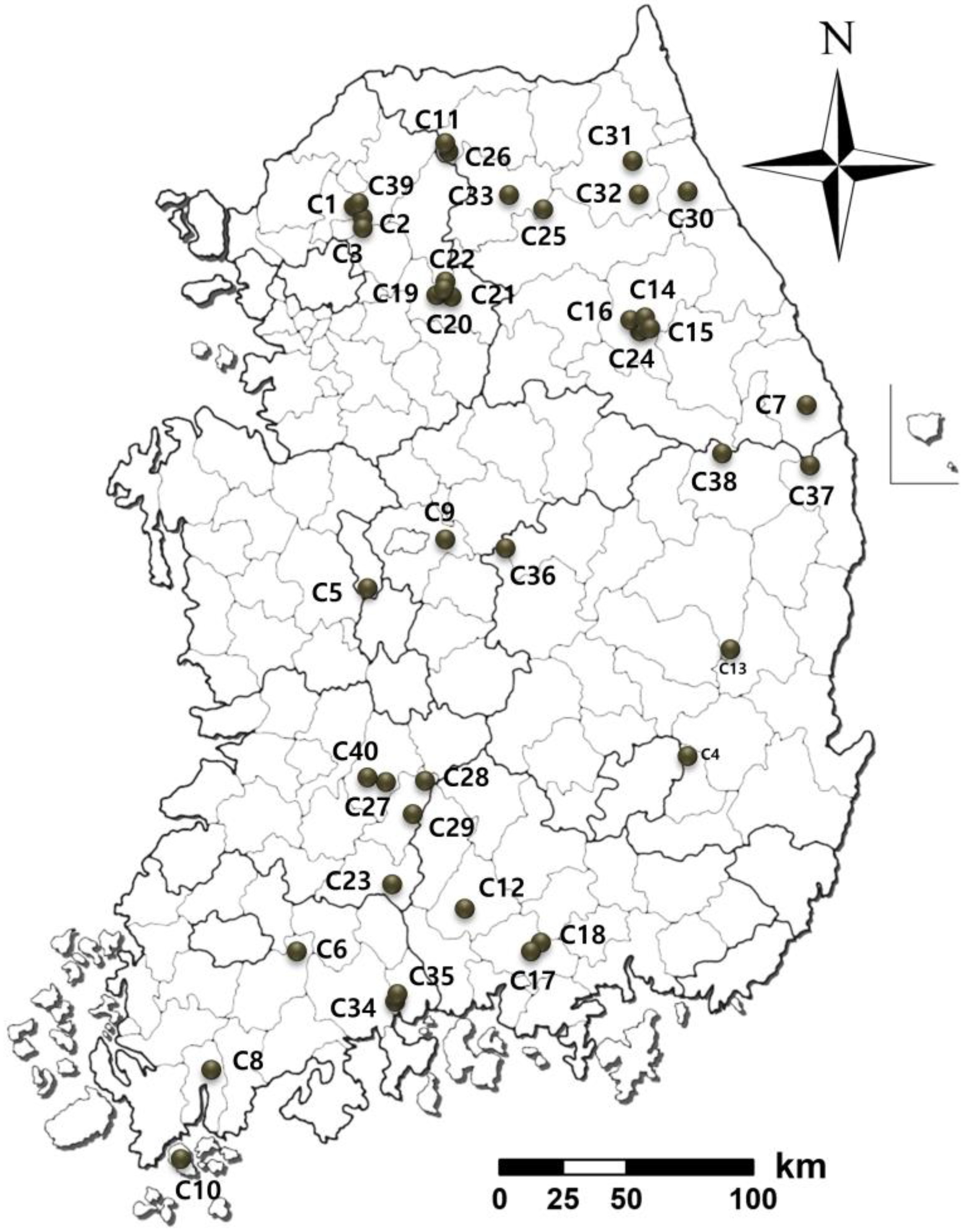
Figure 1. In this study, 40 small forested catchments were used, where water level gauge dams were installed.
Forests 14 01131 g001
Figure 2. Input and output data for developing flood peak predictive model. Six static variables for catchment characteristics and three dynamic variables for meteorological features were used to train the RF models. The warning lead times were 1 h and 6 h, based on the extremely short-term rainfall prediction system of the KMA.
Forests 14 01131 g002
Figure 3. Relationship between the observed and modeled flood peaks. Random forest predictive models were developed with two different warning lead times at (a) 1 h and (b) 6 h.
Forests 14 01131 g003
Figure 4. Flowchart of model building and performance evaluation processes for analyzing the minimum number of flood events required in data collection.
Forests 14 01131 g004
Figure 5. (a) Relationship between the number of flood events used for training dataset (N1; defined in Figure 4) and the predictive performances; (b) 0, 100, 250, 500, 1000, 1500, and 2167 flood events were selected, and the flood data of catchment C3, hypothesized as the ungauged catchment, were added repeatedly to the previous dataset to analyze the predictive accuracy.
Forests 14 01131 g005
Figure 6. Relationship between the number of flood events of 39 catchments and the performance increment ( N S ) . In this instance, data for 205 flood events were confirmed as the required number of flood events for effective flood peak prediction in an ungauged area when an N S value of 0.1 was selected as a criterion.
Forests 14 01131 g006
Figure 7. Distribution of the minimum number of flood events in the collected data to develop an effective predictive model from a total of 7000 iterations. Dark gray indicates a probability of 95% and light gray indicates a probability of 90%.
Forests 14 01131 g007
Disclaimer/Publisher’s Note: The statements, opinions and data contained in all publications are solely those of the individual author(s) and contributor(s) and not of MDPI and/or the editor(s). MDPI and/or the editor(s) disclaim responsibility for any injury to people or property resulting from any ideas, methods, instructions or products referred to in the content.