Patterns of Forest Species Association in a Broadleaf Forest in Romania

Abstract

Ecological patterns of species distribution can reveal essential information on the spatial and functional relationship between species or species and their environment. Various approaches can be used to assess species associations, and our study aimed to compare three methods at different scales: the co-occurrence indices for binary presence–absence data, principal component analysis (PCA) on species abundance and point process analysis. Our goal was to gain a deeper understanding of the species’ co-occurrence patterns and notice if the three methods capture roughly the same spatial distribution trends. Our observational study of the analysed sapling community displayed several positive relationships between species (e.g., the association between ash and linden). However, many relationships were inconsistent across different scales. Furthermore, attraction between species was more prevalent than repulsion. Overall, there is a positive association trend, with more relationships being significantly positive across all scales. This trend is consistent with other recent studies of tree–species interaction. Nonetheless, the results suggest that the scale significantly influences spatial patterns of associations. Positive associations tend to be more prevalent on larger scales, while negative associations are more commonly found on smaller scales, regardless of the analysis method used. While the PCA results are less consistent, the point process analysis allowed us to detect more refined patterns of species associations based on the distance of their interaction. In addition, the binary presence–absence analysis provided solid results, with a coarser spatial perspective but with significantly less sampling effort.

1. Introduction

Ecological patterns of species distribution are of great interest for researchers who aim to decipher and understand the interspecific connections. Moreover, these patterns can reveal essential information on the spatial and functional relationship between species or species and their environment [1]. Due to this particular interest and the large amount of information encapsulated in co-occurrence data, ecological similarity or association studies are widely used in community ecology, assembly ecology, spatial diversity, or ecosystem dynamics [2,3].

The species co-occurrence in a defined space could reveal interspecific associations caused by the functional dependency of specimens and their environment. When two species prefer the same habitat or have similar environmental requirements, there are indications of a positive association. Conversely, if they have distinct ecological needs, negative associations may occur [4]. Furthermore, association relationships between species can also develop as a direct result of biotic interactions. However, a recent study [5] highlighted that researchers should not always link species association or co-occurrence to their ecological interactions.

Various quantitative methods have been developed to assess the ecological resemblance [2] between sites or species composition patterns. Indices of co-occurrence or pairwise association for binary presence–absence data are among the first used and still very popular in assessing ecological resemblance [6,7,8,9]. Researchers use association or co-occurrence metrics on pairs of entities to establish whether their presence is linked or independent and to estimate resemblances or dissimilarities among different data sets. These investigations unveil hidden spatial distribution patterns in ecology, biogeography, biodiversity, epidemiology or evolution [3].

The theoretical framework of binary data metrics was developed at the beginning of the previous century [10]. Nowadays, many indices are still used to evaluate presence–absence associations on the analysed pairs [6,7,11] because they are practical in inferring potential biotic interactions [12]. Despite their wide use, recent studies [3,9] showed that the theoretical framework of these indices has flaws, especially related to species prevalence and scale analysis, which might lead to misinterpretations. Furthermore, the deficiencies regarding significance testing led to diverse and complex approaches: identifying null distribution [12], constructing a null model using simulations [6,11,13] or standardization of counts and indices [6,14,15].

There are more than 80 association indices based on binary data [6,7], and selecting an appropriate one may be provoking. However, most studies orbit around the same indices, and the many reviews and comparisons [7,8,11,14,16,17,18,19] facilitate the selection of the right index [10,13,15,16].

While the binary indices consider the number of shared events (species co-occurrence) and are straightforward to calculate [7,8], the data on species proportions or abundance is not integrated into this evaluation. Having more than two species and adding information on their abundances increase the complexity of the analysis [6]. Therefore, this study also uses a method which incorporates the local species abundance per quadrat. The scale of the analysis can also influence the association patterns of the species [5,19,20]. Many association or co-occurrence studies use quadrats analysis or quadrat sampling [19,21,22].

Species are typically nonrandomly scattered due to intra- and inter-specific interactions and in response to their environment [23,24]. The assumption that spatial distribution patterns meet the condition of randomness within each species limits the co-occurrence indices’ relevance. Therefore, different modern approaches have been developed in recent decades to assess species association based on data mining [25], network theory [3,26,27] or spatial point pattern analysis [24,28,29,30,31].

Among the various approaches, the most common is to investigate species’ spatial patterns using point process analysis through univariate or bivariate Ripley’s K-function [32,33]. Consequently, the present study also integrates the analysis of the spatial distribution patterns of species at different scales through bivariate Ripley’s K-function.

The object of our observational study was a sapling community. We focused on it because biotic interactions in these communities are highly complex and confined to limited spaces [34,35], offering a solid test platform to compare different methods for species association assessments. Although few studies investigated the particularities of juvenile forest communities, shaped by many biotic and environmental factors, we consider the potential practical importance of association patterns not only for the insight into community assembly but also to provide forest restoration directions.

Therefore, in this paper, we examine the patterns of species association in a sapling community using three different approaches: co-occurrence indices based on binary data, local abundance examination by principal component analysis (PCA), and spatial point pattern analysis of species distribution. We aimed to test the three methods by examining species associations at different scales. All three procedures cover the narrative of species interaction and create a picture of forest species association in a sapling community.

Nevertheless, do all methods depict the same picture? Or do the different approaches generate distinct perspectives, which could bind as part of the same scene?

Thus, the main goal of this study is to investigate the forest species association trends in a specific sapling community using different methods and scales to understand the co-occurrence patterns better.

2. Materials and Methods

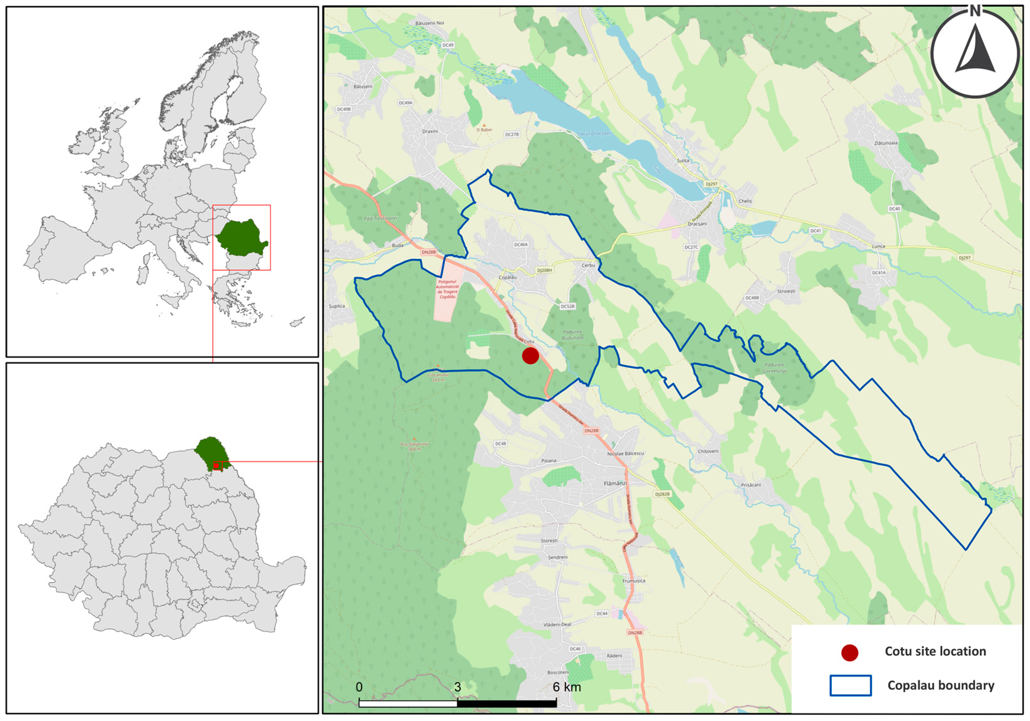
2.1. Study Site

The investigations were carried out at approximately 140 m a.s.l. in a broadleaf forest stand near Cotu village, Botosani County, Romania (47°35′41″ N, 26°51′44″ E) (Figure 1). The climate is temperate continental, with a mean annual temperature of 9 °C and a mean annual precipitation of 560 mm·year⁻¹.

The stand was regenerated using the group shelterwood system, and the final removal cuts were applied six years before installing the sampling plots. In the study area, the seedlings had similar vegetation conditions: the aspect was northeast, the slope ranged between 2 and 4°, and the altitude varied from 135 to 140 m. The soil is classified as greyic phaeozem. We located our study in an even-aged managed forest stand with a representative species composition for this region. Before the felling, the stand composition was pedunculate oak (50%) and hornbeam (30%), with small-leaved lime (10%) and common ash (10%). At the moment of the final removal cut, the stand was approximately 130 years old (130 years for the pedunculate oak and 110 for the other species), and the canopy cover was 0.6. The final cut was synchronised with a relatively abundant fruiting year for oak (but not a fully masting year). More detailed information on the stand can be found in the Supplementary Material (Table S3).

We chose this regular stand type to minimise confounding factors and accurately study the species association from the statistical point of view. Therefore, we selected a case study in an even-aged stand, with consistent regeneration in terms of age and size and representative species composition for this habitat type.

The tree species of the seedlings we found in the sample plots were pedunculate oak (Quercus robur L.), hornbeam (Carpinus betulus L.), small-leaved lime (Tilia cordata Mill.), common ash (Fraxinus excelsior L.), field maple (Acer campestre L.), wild cherry (Prunus avium L.) and sycamore maple (Acer pseudoplatanus L.). However, very few specimens of other species were also identified: dog rose (Rosa canina L.), common dogwood (Cornus sanguinea L.), common hawthorn (Crataegus monogyna Jacq.), and elder (Sambucus nigra L.).

2.2. Data Collection

Within the stand, a homogeneous area with a compact seedling cover was selected, where we set up a network of 10 plots in which all individuals were inventoried. The understory in that area was relatively uniform in size and age, being the last part of the stand that was harvested. The plots were positioned in two rows, with plot limits separated by 50 m. A buffer strip of 100 m was left from the stand boundary to prevent any specific composition irregularities due to the edge effect.

Each rectangular plot of 7 × 7 m was positioned in the field, marked with wood pickets, and delimited with cords. This plot size was chosen for practical reasons, following an evaluation of the saplings’ density and considering the possibility of precise and reliable determination of the individual positions. The species were identified for all saplings, and each individual’s spatial coordinates were determined (x, y). The distances were measured (1 cm precision) from the stem to the abscissa and ordinate of a Cartesian system, with the origin in the bottom-left corner of the plot. We determined the distances in the field using measuring tape sets and a Leica DISTO laser distance metre. The measurements were carried out successively for one-metre sections of the plot, delimited by cords and precise markings.

All the seedlings were sampled in the ten plots, regardless of species, resulting in approximately 7200 saplings being inventoried in all the plots. However, to avoid a “dilution effect’’ [36], only the data from 7171 individuals were used in further analysis, belonging to the seven species with a percentage above 1% in the seedling composition. We examined the species association for all species where this was theoretically possible, and only dog rose, common dogwood, common hawthorn, and elder were excluded due to their very low abundance.

2.3. Data Analysis

The proposed framework of this study involves making inferences on species association in sapling communities using different methods and scales.

The sampling volume is crucial in identifying association patterns [5], therefore, the analysis employed an extensive data set for 7171 individuals, which implied a significant sampling effort and a substantial computing amount. To efficiently use the large data volume, we performed additional processing.

Addressing the scale issue—One method utilized is spatially explicit (point process analysis). Nonetheless, incorporating different scales in the other two methods, the binary indices of co-occurrence and the PCA, required a supplementary space partitioning of the ten analysed plots. Therefore, we split the data from the ten sampling plots into seven different variants of smaller quadrats to address the problem of spatiality. Then, we quantified the presence–absence data for the binary analysis and the abundances of the species (for PCA) in each quadrat.

The scale of the analysis profoundly impacts the ecological spatial patterns [5,19,20,37], and various methods are applied to integrate the spatial perspective. For instance, the quadrat approach is frequently used to study the scale influence on species association patterns [19,21,22]. Finding a suitable sampling size for characterizing community spatial interactions is difficult. Interpreting species association is challenging in large quadrats because the spatial patterns can be diffused, and in small quadrats, it is possible to record only a few interactions between species [20,21]. Therefore, we used several different quadrat sizes to reveal possible hidden association patterns. In our study, the regular 7 × 7 m quadrats were divided into 196, 49, 25, 16, 9, and 4 smaller quadrats corresponding to other six scales, of 0.5 × 0.5 m, 1 × 1 m, 1.4 × 1.4 m, 1.75 × 1.75 m, 2.33 × 2.33 m, and 3.5 × 3.5 m, respectively.

For each scale and quadrat, we assessed the species’ local abundance. Further, based on the saplings’ x and y coordinates, a function was implemented for each individual to compute the number of the quadrat it belongs to (the code is available in a publicly shared repository). This procedure was repeated for all quadrats’ scale configurations. Then, the quadrats with no seedlings of any of the seven analysed species were removed from further analysis.

The binary analysis of co-occurrence—The binary indices are explicit in their evaluation, based on the number of species co-occurrence in the same area. The joint presence of species could be interpreted as a meaningful ecological parameter [38]. However, selecting a relevant binary index of co-occurring may be challenging, considering the large number of indices [6,7].

In our analyses, we selected the Jaccard index [10], a classical index of co-occurrence that does not incorporate negative matches (quadrats where both species are missing). This is one of the most expressive and frequently used indices, which is often recommended [13,15,16]. Its value ranges between 0 and 1, with values close to 0 implying highly negative associations and those near 1 implying highly positive associations between species. The Jaccard index (J) was used in R-mode to measure between-species associations and not in Q-mode to measure beta diversity [2,20].

The index calculation is similar to the binary indices, based on the abcd matching components [19] specific to contingency tables.

The mathematical formula is J = a/(a + b + c), where a represents the number of shared presences in the same area; b is the number of presences of the first species, and c is the number of presences of the second species. The J index is a binary index that does not consider joint absences (negative matches), making it more reliable in analysing communities with an unbalanced distribution of species percentage [6].

The index values were calculated by implementing a function (the code is available in the supplementary material) that evaluates the previous formula by counting and interpreting the data related to the presence of the analysed species in each quadrat. The function was employed separately for every scale configuration. Presence–absence data were obtained from the local abundance data sets calculated per quadrat for all seven scales.

The significance of the Jaccard index was assessed at a significance level of 0.05, using computed lower and upper critical values [15,39].

The principal component analysis—The local species abundance per quadrat was analysed using PCA, considering that binary indices do not include species proportions or abundance data. Utilising this available data, we performed PCA to obtain a comprehensive picture of species association preferences.

The principal component analysis is a statistical technique that condenses large volumes of data into smaller components, which makes it more straightforward to visualize and understand [40]. The procedure captures the maximum information in a data set by re-aligning the axis in an n-dimensional space to obtain most of the variance in the data [41]. Any two principal components create a model plane on which all the observations are projected, making it easier to observe the layout of the examined data set [42]. The entities clustered close to each other reveal positive connections, having similar profiles, whereas those far from each other are dissimilar. PCA is a versatile Euclidean-based ordination method, widely used in ecology studies to analyse community data [2], and occasionally utilised in investigating the association of species [43]. Furthermore, the data on the abundance of species is also frequently integrated into PCA analyses that examine the relationships between temporal trends in abundance and suits of functional traits [44,45] or species–habitat associations [34,46]. In our study, all the different scales and species analyses were performed using R [47].

Spatial point process—The previous methods are distance-independent, and we used quadrats of different sizes to deliver spatial relevance to the analyses. The point process approach is natively spatially explicit and have been used for several decades in ecology to analyse spatial distribution patterns [32,33,48,49]. For example, Ripley’s K (t)-function is a cumulative distribution function that adds the expected number of events discovered within a specified distance of each point (t) while increasing the radius of concentric circles [32,33,49,50]. In bivariate analysis, an extension of Ripley’s K-function is used to determine if species exhibit spatial attraction, independence, or repulsion [48,49,51,52,53]. This approach is one of the most frequently used for examining the spatial dependency between plant species [24,25,28,29,30,31,54,55]. Therefore, in this paper, we also used the bivariate spatial point process to infer the spatial association within sapling communities.

For the bivariate analysis, two K(t) estimators are computed (Equations (1) and (2)), counting the neighbours of each analysed species: K₁₂ describes the pattern of species 2 in relation to species 1, and K₂₁ the pattern of species 1 in relation to species 2.

$${\tilde{K}}_{12}\left(t\right)={\left(n_1{n}_2\right)}^{-1}\cdot A \sum \sum w_{ij}^{-1}{I}_t\left(u_{ij}\right)$$

(1)

$${\tilde{K}}_{21}\left(t\right)={\left(n_2{n}_1\right)}^{-1}\cdot A \sum \sum w_{ji}^{-1}{I}_t\left(u_{ji}\right)$$

(2)

where, n represents the number of individuals for each species, A is the analysed plot area, u_ij is the distance between individuals i and j, I_t is a counter of the distances, and w_ij is a weighting correction factor, compensating the edge effects [49,50,54]. The estimators calculate the expected number of individuals of one species within a radius t of an arbitrary individual of the other species [53]. Both estimators were linearly combined into a weighted single mean estimator (Equation (3)) [48,51], and the local weighting method [32,50,52] was used to calculate the edge corrections.

$${\widehat{K}}_{12}\left(t\right)={\left(n_1+n_2\right)}^{-1}\cdot [n_2\cdot {\tilde{K}}_{12}\left(t\right)+n_1\cdot {\tilde{K}}_{21}\left(t\right)]$$

(3)

To stabilize the variance of the K(t) function, we used the L-statistics transformation of Besag [52,53,54], which also facilitates the visual interpretation of the results (Equation (4)).

$${\widehat{L}}_{12}\left(t\right)={\left({\widehat{K}}_{12}\left(t\right)\cdot {\pi }^{-1}\right)}^{0.5}-t$$

(4)

Investigating spatial association patterns in bivariate spatial point processes may require different null hypotheses: population independence or random labelling. In this situation, considering we analyse between-species interactions, the adequate null hypothesis is population independence (L₁₂(t) = 0) [54], making it possible to test whether interactions between species have significantly increased their spatial dependence. The positive values of L(t) indicate attraction, and the negative ones indicate repulsion among the spatial pattern of the analysed species [52]

To assess the statistical significance of L(t) values, we used a randomisation method based on 1000 Monte Carlo simulations of random coordinates of species and toroidal shifts [52,53,54]. Using the simulation data, we generated a critical confidence envelope at a significance level of 0.05 (p ≤ 0.05) for the L(t) function. Considering the independent null model, the function values within the confidence intervals indicate no interaction between species, while the values outside this range reveal significant associations at the corresponding distance. Individual charts were created for each species’ relationship and plot. The positive values of L(t) indicate attraction, and the negative ones indicate repulsion among the analysed species (Figure 2). In the supplementary data, all the individual graphs are presented (Figures S29–S48).

We progressively incremented the distance t by 5 cm to 350 cm. The maximum value was half the size of the side of the plot to avoid biases for large values of the distance [49,50,52]. We also performed an overall test of complete spatial randomness (CSR) using the Cramer-von Mises test to assess the overall significance of patterns over the full range of t, incorporating the squares of the L(t) function deviations from expected values [49,52,53]. The ranking of the L-statistic considering the number of simulations was used to obtain the significance level of probability using the Haase method [53], the null hypothesis being rejected at the p < 0.05 level.

For the seven species, 20 out of 21 pair–species relationships were analysed, one of the relationships (Pa–Ap) being excluded due to the low number of trees in the analysed plots. In addition, several other plots were also eliminated in the case of point process analysis from particular species analyses because they did not meet the requirement of having at least ten individuals of each species in a plot.

In order to consolidate the information about the significant ranges of positive or negative association, summarising bar charts were designed for each species’ relationship. Therefore, only the ranges with the significant association are transposed in the bar chart (Figure 3). Additionally, the plots with a significance level of probability lower than 0.05 for the Cramer-von Mises test were highlighted; they are marked with circles.

Figure 2 and Figure 3 illustrate an example of data integration of the individual graphs into a summary chart that displays the consolidated information for the Cb–Tc relationship. The supplementary data presents all the summary bar charts (Figures S9–S28).

The bivariate analysis, including simulations and L-statistics, was conducted using SPPA ver. 2.03 [56].

The tree species were abbreviated in the analyses: Qr—Quercus robur, Cb—Carpinus betulus, Tc—Tilia cordata, Fe—Fraxinus excelsior, Ac—Acer campestre, Pa—Prunus avium, and Ap—Acer pseudoplatanus.

The other source code mentioned in this section and used for the plots’ quadrat partitioning, the binary co-occurrence analysis, and the PCA is publicly shared (https://github.com/cpalaghianu/saplings, accessed on 15 May 2023).

3. Results

3.1. The Analysis Based on Binary Indices

We identified seven species with a percentage above 1% in the seedling composition: Carpinus betulus—55% (Cb), Quercus robur—16% (Qr), Tilia cordata—11% (Tc), Fraxinus excelsior—9% (Fe), Acer campestre—6% (Ac), Prunus avium—2% (Pa) and Acer pseudoplatanus—1% (Ap). The density of the saplings per square metre was 14.80, with a coefficient of variation of 20% between the plots. Even if pedunculate oak dominated the parent stand (Table S3), hornbeam is the species that dominates the regeneration cohort. The rarity and low intensity of masting events for oaks in the area might partially explain this situation.

All the relationships between the seven species were analysed, and the value of the Jaccard index was calculated for different quadrat sizes using presence–absence information from the local abundance data. The higher values indicate positive associations between species, while the lower infer negative associations. The significance and interpretation of the associations for the 21 pairs of two species are presented in

Table 1. Jaccard index significance and interpretation of species associations for different quadrat sizes.

Qdrt. Size	Cb–Pa	Cb–Fe	Cb–Ac	Cb–Ap	Cb–Qr	Cb–Tc	Pa–Fe	Pa–Ac	Pa–Ap	Pa–Qr	Pa–Tc
7 × 7 m	1.000	1.000	1.000	0.700	1.000	1.000	1.000	1.000	0.700	1.000	1.000
3.5 × 3.5 m	0.800	0.950	0.925	0.525	0.950	1.000	0.795	0.816	0.432	0.842	0.800
2.33 × 2.33 m	0.567	0.744	0.722	0.322	0.922	0.967	0.532	0.487	0.250	0.576	0.551
1.75 × 1.75 m	0.381	0.638	0.594	0.238	0.813	0.850	0.336	0.322	0.165	0.404	0.387
1.4 × 1.4 m	0.272	0.548	0.488	0.160	0.740	0.732	0.235	0.250	0.091	0.278	0.287
1 × 1 m	0.183	0.384	0.337	0.089	0.606	0.524	0.181	0.196	0.063	0.201	0.185
0.5 × 0.5 m	0.051	0.187	0.131	0.031	0.284	0.203	0.045	0.048	0.000	0.051	0.056
Qdrt. size	Fe–Ac	Fe–Ap	Fe–Qr	Fe–Tc	Ac–Ap	Ac–Qr	Ac–Tc	Ap–Qr	Ap–Tc	Qr–Tc
7 × 7 m	1.000	0.700	1.000	1.000	0.700	1.000	1.000	0.700	0.700	1.000
3.5 × 3.5 m	0.875	0.475	0.900	0.950	0.568	0.974	0.925	0.553	0.525	0.950
2.33 × 2.33 m	0.610	0.215	0.705	0.750	0.306	0.721	0.727	0.318	0.303	0.889
1.75 × 1.75 m	0.470	0.167	0.589	0.630	0.198	0.585	0.604	0.273	0.234	0.739
1.4 × 1.4 m	0.385	0.113	0.464	0.546	0.117	0.476	0.473	0.172	0.155	0.586
1 × 1 m	0.262	0.073	0.297	0.413	0.071	0.340	0.281	0.110	0.066	0.382
0.5 × 0.5 m	0.102	0.018	0.124	0.198	0.006	0.134	0.092	0.026	0.019	0.128

Note: The grey-shaded cells highlight the significant values at a significance level of 0.05. Dark grey cells indicate significant positive associations, while light grey cells indicate significant negative associations.

, the values being differentiated by the colour of the cells.

Most relationships between species are statistically significant. Nearly 80% of the associations are significant from 147 relationships analysed at different scales. About 48% of the total relationships reveal significantly positive and 31% significantly negative associations. The positive associations are mainly found in larger quadrats, over 1.75–2.33 m, while the negative ones are encountered at a smaller scale, in quadrat sizes below 1.4–1.0 m. Almost all Jaccard index values for the 0.5 m quadrats reveal significant negative associations, with 20 relationships out of the 21 analysed.

There is a relative consistency from the spatial point of view of the association behaviour of the species because some relationships are predominantly positive, while others are mostly negative, regardless of the scale. For example, the associations Cb–Tc, Cb–Qr, and Fe–Tc preserve a significant positive association on six of the seven spatial scales analysed.

In contrast, the associations Cb–Ap, Pa–Ap, Fe–Ap, Ac–Ap, and Ap–Tc preserve a significant negative association on at least four of the seven spatial scales analysed.

Large differences between the co-occurrence Jaccard index for the species pairs were recorded. In order to emphasise the general behaviour of the species’ relationships for all seven scales, we conducted a graphical cumulation of the values of the Jaccard index to rank the intensity of the association between the different pairs of species (Figure S1).

3.2. The Analysis Based on the Relationship between Quadrat-Specific Abundances

The second stage of examining species association trends was based on the principal component analysis, which clusters species on abundance features. Compared to the co-occurrence index analysis, the PCA incorporates additional information about local species abundance per quadrat.

The principal component analysis was performed to identify tree species associations that explain most of the variation between the individual quadrats of the same size. The analysis helps us visualise the strongest trends in the dataset, considering PCA groups variables (in this case, species) rather than observations (local abundances).

The investigation used seven tree species and seven different sizes of quadrats. The results reveal species clusters with similar abundance profiles. Therefore, species close to each other might suggest positive associations, whereas those far from each other might be dissimilar.

The graphical output is presented in Figure 4 for two-dimensional variants (0.5 × 0.5 and 7 × 7 m quadrats), and the charts for all seven quadrat sizes can be found in the supplementary data section (Figures S2–S8).

Examining the PCA plots allows us to identify specific clustering trends. Thus, the positive association between Fe and Tc species is evident in all the seven charts. At the same time, although less consistent for all quadrat sizes, the clusters between the species Ac–Pa and Ac–Qr might suggest a similar affinity.

The correlation values between species and the principal components indirectly support the visual observations on between-species associations. For example, in the quadrat 0.5 × 0.5 m, the first principal component (PC1) has the highest positive correlation values employing Tc and Fe species (Table S4), while Qr and Cb are weakly correlated. Therefore, Tc and Fe species explain most of the variation in the species abundance amongst quadrats.

On the other hand, the second principal component (PC2) has the highest correlation to Cb (positive) and Qr (negative) species. Thus, these species contribute the most to species abundance variance for PC2 (Figure 4). The pair–species correlations and the explained variance of PCA for all the seven quadrat sizes are summarized in Table S4.

Scrolling the results and noticing PC1’s high correlation (negative or positive) with Fe and Tc species, we consolidate the visual observations on the positive association between Fe and Tc species. Similarly, examining other species’ associations and correlations with PC2, the higher and similar correlation values in the case of the pairs Ac–Pa and Ac–Qr also confirm the clustering displayed in the biplots.

These findings are consistent with all quadrat dimensions in the case of PC1, considering the Fe–Tc relationship, while there are several differences in the case of PC2. In this case, the Ac–Qr association is evident for quadrat sizes larger than 1.75, while the Ac–Pa relationship is noticeable only for 1 × 1 m and 1.4 × 1.4 m quadrats.

The quadrat size also determines substantial differences in the variance explained by the principal components. The variance increases with the quadrat’s dimensions (Table S4), as it is related to the number of analysed quadrats.

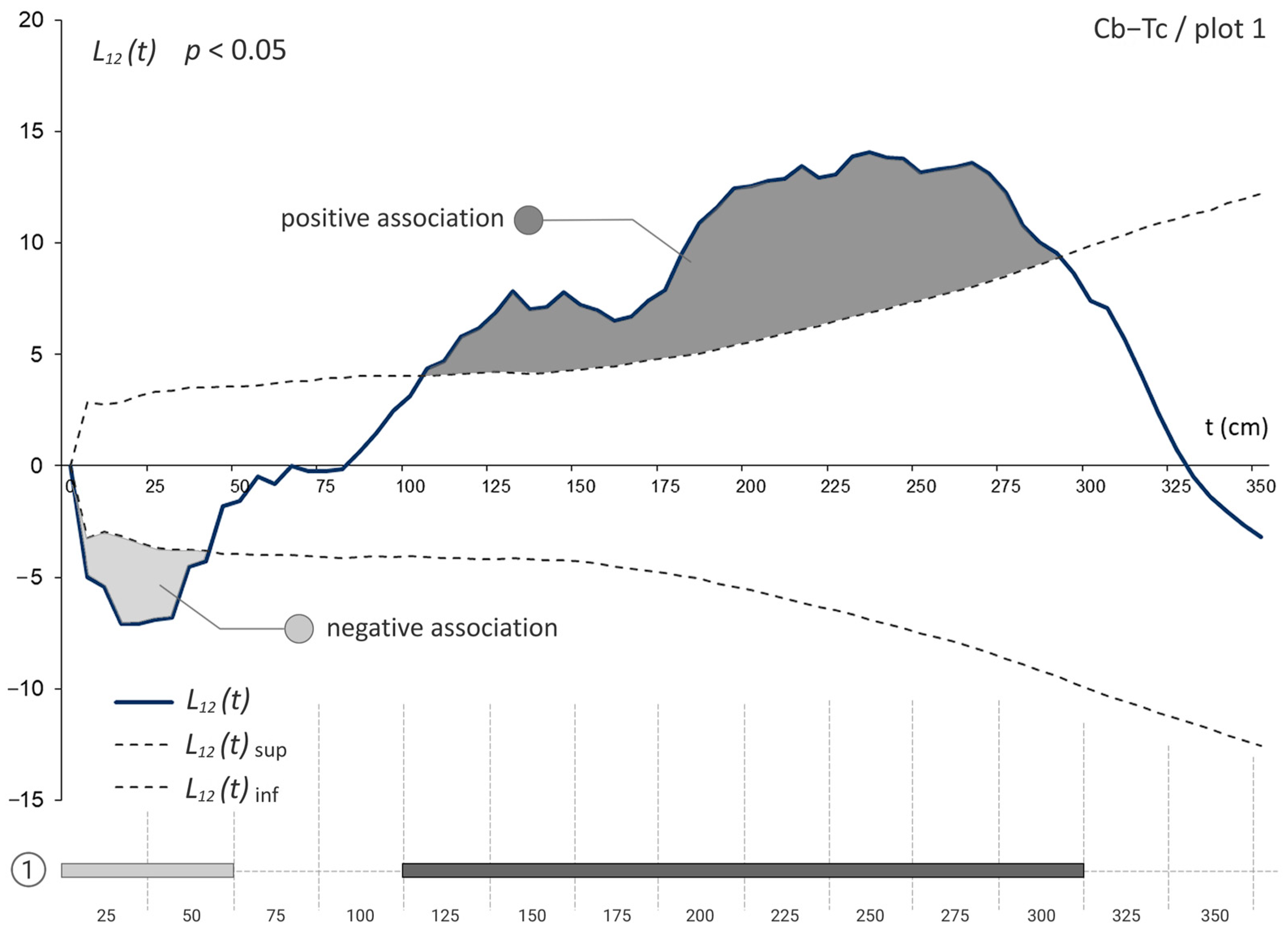
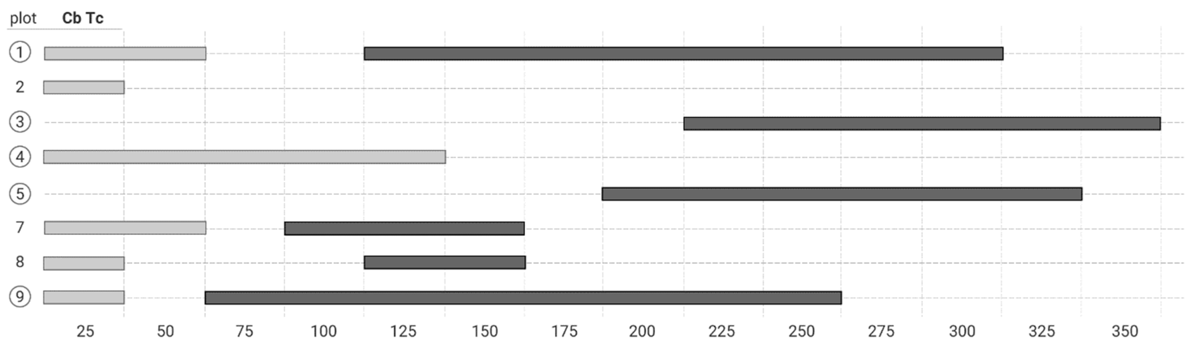
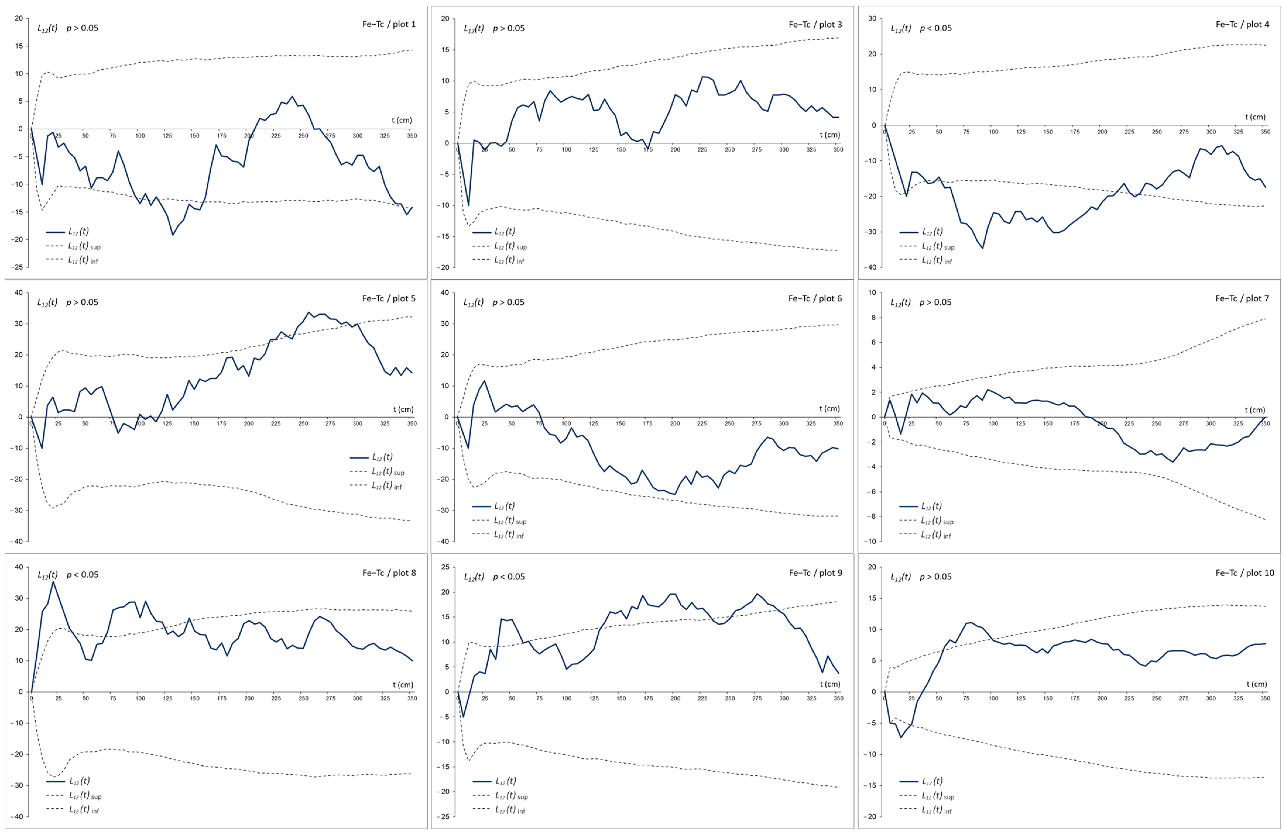
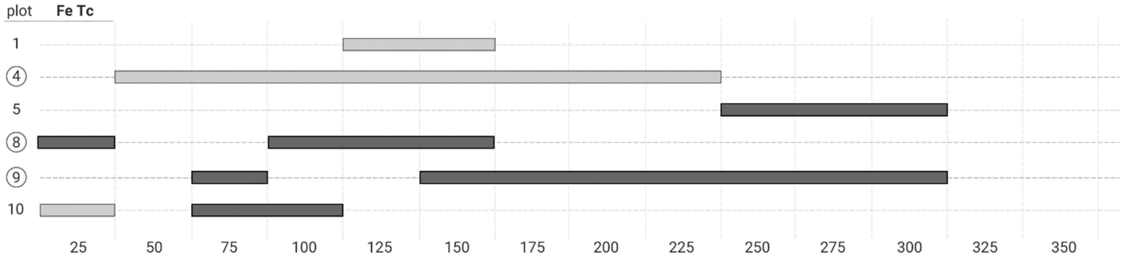
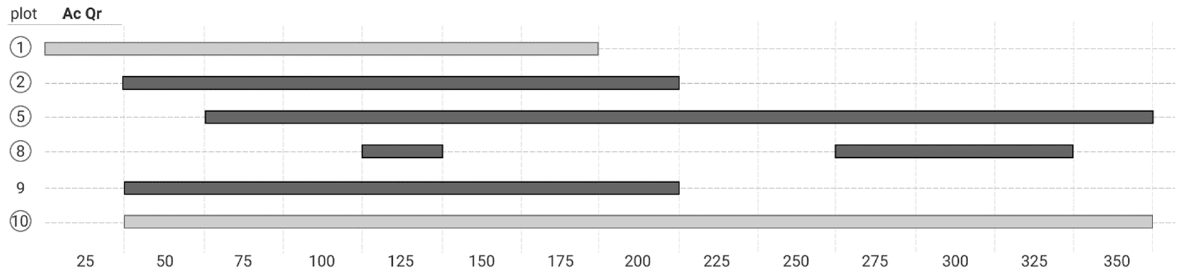
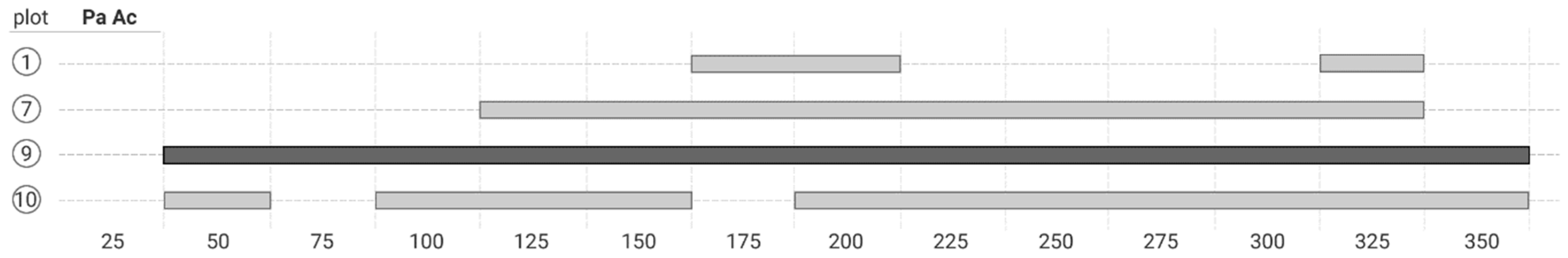
3.3. The Bivariate Analysis

Another detailed perspective provided in this observational study was assembled using a spatially explicit approach based on L-statistics of point process analyses. This method reveals the spatial distribution patterns of the species at finer scales without using quadrats of different sizes. In this case, the analyses are conducted by plot, wherein each relationship between species is analysed separately for all the ten plots.

The species association trends analysed using point process analysis seem less consistent compared to the previous methods of investigation. In this case, the analyses are no longer independent of the plot but are confined to a particular space defined by one of the ten plots. Considering that the plots’ variability is high, inconsistent trends of associations between species appear more often.

For instance, the Fe–Tc relationship, one of the most consistent relationships in the PCA analysis (Table S4), is relatively variable for different plots (Figure 5). The distinct trends observed in the individual graphs are condensed in the bar graph showing only the significant association ranges (Figure 6). Different association trends for the same species relationship can be unveiled between the analysed plots and substantially different patterns even within the same plot (plot 10). Considering only the relevant plots for which the total Cramer-von Mises test has a significance level of probability lower than 0.05, the association tendencies are predominantly positive between the two species (Fe–Tc). In plots 8 and 9, the significant trends of the positive association are discontinuous on intervals up to a maximum of 300 cm. However, in plot 4, the significant trend indicates a negative association on a continuous interval between 50 and 225 cm.

Summary graphs were displayed for two other relationships that indicated possible positive association tendencies following the PCA analysis. First, the Ac–Qr positive association was suggested for quadrat sizes larger than 1.75 m. The summarising chart (Figure 7) greatly supports this indication, considering that significant trends of a positive association between the two species can be observed in four of the six plots.

Another positive association was suggested in the PCA analysis for the Pa–Ac relationship for 1 × 1 m and 1.4 × 1.4 m quadrats. However, the summary chart for this species relationship (Figure 8) does not align with the PCA findings. The significant ranges also display negative association trends between the two species, although there is a significant positive association on a continuous interval between 50 and 350 cm in plot 9.

The analysis of the significant ranges of associations in the condensed graphs (Figures S9–S28) reveals several consistent types of relationships between species. Several relationships, such as Cb–Fe (with positive ranges in all the analysed six plots), Fe–Ac, Fe–Qr, Ap–Qr and Pa–Qr, suggest mostly positive associations. In contrast, others, such as Qr–Tc and Ac–Tc, are mostly negative.

The point processes analysis allows the detection of more refined patterns of associations depending on the interaction distance between the species. In some cases, the two types of association, positive and negative, can coexist, even within the same plot, but at a different spatial scale. Thus, a case of mixed association is the Cb–Tc relationship (Figure 3), which is mostly negative up to 75 cm and predominantly positive above 100–125 cm.

4. Discussion

Although the studies on the community species composition have a strong theoretical component, the findings can also be of practical use as a decision-making tool for partitioning the mixture of species used in planting actions and in providing forest restoration directions. [57]. Most previous studies on species association focused on species–habitat associations and not on between-species associations [2,58]. Furthermore, many studies concentrated on tropical and subtropical forests [29,57,59,60,61]. Relatively few analyses were conducted on the association of seedlings of forest species [35,62,63,64] and even less focused on deciduous species from temperate regions. Consequently, the current study focuses on a topic that has received less attention and uses an approach involving three different methods to determine to what extent their perspectives can be integrated into a single “scene”.

An important aspect of our study which we want to highlight is that we considered the sapling community to be homogeneous in size (Table S2) and age. We did not systematically investigate the age of all the seedlings. However, we conducted several observations in the field which suggested that the age differences between the seedlings were limited. The installation of the first cohort significantly reduced the chances of survival of the new seedlings, considering the limited space and access to light. Studies on deciduous [65] and coniferous species [66] showed that generating a new cohort of saplings is challenging due to low light availability, even for shade-tolerant species.

4.1. Specific Co-Occurrence Patterns

The three methods used in this investigation are different in terms of sampling, collection, analysis and interpretation of data. Undoubtedly, these differences could lead to distinct results. Nevertheless, do they offer conflicting perspectives? Or do we still have a glimpse of the same associations and co-occurrence patterns of species. To better understand the results, we briefly compare the specific elements of each analysis.

The Jaccard index is a classic binary index based on the number of species co-occurrence in a set of quadrats, used in R-mode to measure between-species associations [2]. Although the evaluation using this method directly provides a value that defines the “intensity” of the relationship between two species, the quantitative assessment is based on binary data, which inevitably leads to a loss of information [57]. Therefore, even if it uses the same framework of quadrats of different sizes, the PCA incorporates additional information related to species abundance to complete the binary co-occurrence analysis’s missing information. The method provides a visual synopsis of the predominant association trends, the intensity of these relationships being indirectly appreciated through species correlation with the principal components [40]. Quadrat approaches are characterized by limited spatiality and neighbourhood, being confined to a shape of a certain size, but the last technique we used escapes this limitation. Point process methods have come be more frequently used in forest ecology [67] because these methods have a continuous perspective of space. Furthermore, the relative intensity of the bivariate spatial associations could be evaluated using the ratio between the bivariate function and the associated confidence envelopes [64].

Analysing the results, we observe that many species’ co-occurrence patterns are common to all the three methods we used.

Focusing on the Jaccard index values, almost 80% of the associations identified are statistically significant. In addition, 48% of the total relationships were significantly positive, and 31% were significantly negative. Unfortunately, we do not have the means to objectively compare this predominantly positive trend with the results provided by other methods, so we will compare several specific relationships. In the binary analysis of co-occurrence, some relationships have a relative consistency from the spatial point of view, highlighting a significant positive association on six of the seven spatial scales analysed: Fe–Tc, Cb–Qr and Cb–Tc (Table 1). The PCA also highlights the positive association Fe–Tc as the relationship that visually stands out the most (Figures S2–S8). The cumulative variance explained by the first two eigenvalues are presented in the Supplementary Materials (Table S4). The bivariate analysis is not as pronounced or consistent as previous methods in highlighting this affinity on the entire spatial range, but positive associations are present in four of the ten plots (Figure 6).

Our research goal was not to examine the causality mechanism leading to species associations, considering many standard parametric and nonparametric techniques that presume independence among non-independent sample units are inappropriate and may produce misleading inferences [68,69,70]. However, the connection mentioned above might suggest that it was not competition for resources that shaped the pattern. Instead, the two species occupy unique niches facilitating their presence [4]. Additionally, the spatial segregation hypothesis [71] can explain positive associations between species, especially on a small scale. The hypothesis considers that intraspecific aggregation boosts the importance of intraspecific competition, creating a mechanism that improves local coexistence and shapes diverse species communities [72]. Another possible explanation might be offered by the species herd protection hypothesis, which suggests that heterospecific neighbours can facilitate coexistence by containing the transmission of species-specific pests and pathogens [35,72,73,74].

Another consistent relation from the binary co-occurrence analysis, Cb–Tc (Table 1), is not so obviously highlighted in the PCA (Figures S2–S8). However, this association is consistent with the bivariate analysis performed using the L(t) function. Thus, the Cb–Tc relationship is predominantly positive above 100–125 cm in six out of the eight analysed plots (Figure 3). Furthermore, highlighting another similarity, both the Jaccard index and L(t) function reveal the same type of mixed association, that is, negative on a small scale and positive on a large scale for the Cb–Tc association.

Other relationships also show similar patterns for binary co-occurrence and bivariate analysis, such as Cb–Fe and Fe–Qr, with predominantly positive trends. Furthermore, several associations, such as Pa–Fe, Pa–Qr, or Fe–Ac, are positive only for the second half of the dimensional scale. Finally, others species-couples display a partial similarity, as shown in the case of bivariate analysis less constantly, only at specific intervals.

We also found similarities in the negative relationships between species. For instance, the Jaccard index predominantly shows negative associations at the smallest scale of analysis (0.5 × 0.5 m quadrats), results partially supported by the bivariate analysis. Our findings are consistent with other studies, which found small-scale negative associations [61,64,72]. However, the rest of the negative relationships are relatively rare, and the ones encountered at larger scales could be interpreted as a result of environmental filtering at greater scales [61].

However, there are other relationships with considerable differences or mismatches between the three methods. Unfortunately, no comparative studies are available to compare the three methods, but we can suggest some explanations. We used three profoundly different methods considering the data sampling and the interpretation of spatiality. First, the point process analysis has a continuous perspective of space, and the differences between scales and patterns are not as sharp as in the case of quadrats. There is a quadrat limitation considering that part of the information about neighbours of individuals near the limit of a quadrat is lost [46]. Second, the sample sizes of quadrat-based analysis differ from the distance ranges used in bivariate analysis. Moreover, in the case of the bivariate analysis, the evaluation is performed per plot, and the variation of species composition of each plot (Table S1) can explain some inconsistencies across plots. Furthermore, as many studies indicate, the co-occurrence indices, such as the Jaccard index, are sensitive to the prevalence of the entities [3,11,12,27,38,70]. Additionally, the performance of co-occurrence analyses is lower in complex communities with a large number of species [70].

Sapling communities are complex and shaped by many biotic and environmental factors. That is why a high heterogeneity at a small scale can influence the pattern of the spatial distribution of species. Although the species composition of the regeneration community is similar in the study area, the results of the analyses might be determined by the species–environment interactions rather than directly by relations between species [75]. For example, different characteristics of soil and light availability on seedlings among species can be found [62] or various pests and pathogens can be found [74].

The mixed results obtained using the different methods are easier to observe in the case of bivariate associations, which are very sensitive at finer spatial scales. In these cases, our data show significant positive and negative relationships on different ranges, but no general trend of association or repulsion is evident. However, our results are similar to other studies in which similar fluctuations were observed, and no distinct trend was confirmed [55,64,72,75]. Furthermore, Zhou [72] suggested that according to the low-frequency hypothesis [76], ecological dominance might influence the spatial distribution patterns of species because dominant individuals have more frequent interactions than others. Although it is a more frequently encountered problem in biodiversity studies [77], we acknowledge that sampling issues related to different scales can also impact the results of species association investigations. For example, Legendre and Legendre [2] suggested that it is more instructive to compare dominant or abundant species than rare taxa because the latter, having low frequencies of occurrence, are generally inadequately sampled. In our study, the hornbeam (Cb) has a disproportionate weight (55%) compared to the other species in the analysed sapling community. Possibly as a result of ecological dominance, hornbeam (Cb 55%) is found in many of the positive associations, while sycamore (Ap 1%) is in most of the negative ones, as other rare species. To obtain a more comprehensive understanding of species interactions, we included information about the species composition of each plot in the supplementary material (Table S1). This information may partially explain some of the negative associations between species in specific plots, considering that infrequent species might experience sampling issues due to their low frequency of occurrence.

To conclude, the relationship between binary co-occurrence analysis and bivariate analysis appears more solid, with certain overlaps and common points of view. There are more similarities between these two methods compared to PCA. However, further investigations might develop thorough tests and analyses to reveal additional similarities. Thus, PCA is a flexible distance-based ordination method that can confirm and provide solid results in other circumstances [2,43], but for this particular study, the outcomes overlapped to a small extent with the ones provided by the other methods. The binary co-occurrence analysis provided consistent results across different scales, and the L(t) bivariate function emphasised detailed trends of species association at different scale levels.

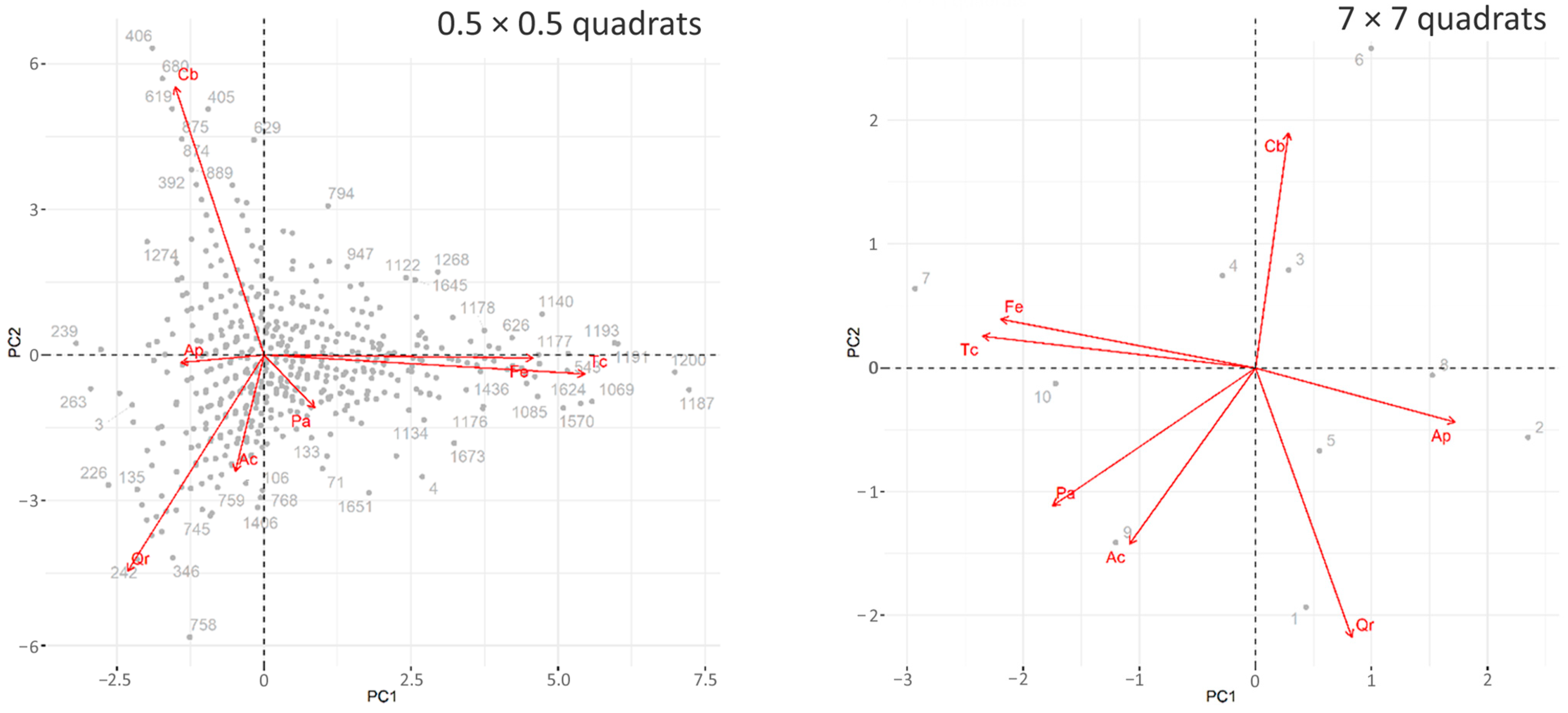
4.2. Co-Occurrence Patterns at Different Scale

Investigations of the spatial distribution of individuals, processes or phenomena are undoubtedly affected by the scale of the analysis [37,77,78]. Bivariate spatial point process analysis is a native spatial analysis method and a robust tool for estimating species co-occurrence patterns [61].

However, quadrats of different sizes with presence–absence data for the binary co-occurrence analysis and local species abundances for PCA were used in this investigation to obtain spatial relevance for these analyses. The quadrat analyses were performed at seven different scales (0.5 × 0.5 m to 7 × 7 m) to quantify the associations of the species. The quadrat sizes were chosen in a progression that would allow recording relevant changes in the association patterns and also considered the possibility of the precise division of the side length of the plot. Individuals are most likely to interact with their closest neighbours on a small scale. At the same time, environmental filtering might extend beyond the neighbour’s scales, generating different association patterns [61]. Considering the high sapling density, the interaction ranges are limited in space. Large sampling cells or quadrats may not facilitate the detection of the spatial dependency present at smaller scales [20].

On the other hand, at small scale, we might find more positive species associations if there are local concentrations of regeneration because of dispersal limitation [79]. Moreover, small quadrats could also be biased toward more negative associations if they are small enough to host a reasonable number of individuals or species. In contrast, the large quadrats will extend over several microhabitats with diverse species compositions. Such quadrats could contain species too far from each other to connect, affecting the biotic interactions and making the interpretation of species associations difficult [21].

The binary Jaccard index provides a specific value defining the intensity of the relationship between two species, which offers an advantage in comparing the values obtained at different dimensional scales (Table 1). The PCA intensity of the relationships can be visually estimated or indirectly appreciated through species correlation with the principal components (Table S4). However, the rarest species have the smallest eigenvalues, and the contributions of these species to the relevant principal components are small. Therefore, PCA results might be affected by inaccuracies generated by the low abundances of rare species [43]. Additionally, in the case of bivariate analysis, the L(t) function provides continuous values over the analysed interval (0–350 cm) that can be easily compared between different distances (Figures S29–S48).

We found a relative coherence from the spatial point of view for species association analysed using the Jaccard index. Nearly all pairs of species were negatively associated at the smallest scale (0.5 × 0.5 m), with 20 significant negative associations out of 21. The maximum number of positive associations was 19, recorded for the 3.5 m quadrat size (

Table 2. The number of significant positive and negative species associations at different scales.

Quadrat Size	0.5 m	1.0 m	1.4 m	1.75 m	2.33 m	3.5 m	7 m
no. of positive associations	0	3	9	10	15	19	15
no. of negative associations	20	12	8	5	1	0	0

).

Overall, there is a positive association trend, with 71 significantly positive relationships and 46 significantly negative from the 147 relationships analysed on the seven scales. This trend is consistent with other recent studies, which found that positive interspecific interactions are more common than negative associations in tree species communities [79]. However, the positive associations are mainly found at a larger scale (beyond 1.75–2.33 m), and the negative ones at a smaller scale (below 1.4–1.0 m). This dispersal of species association trends at different scales (Table 2) might provide helpful information for researchers who want to focus on a specific type of relationship.

For the Jaccard index analysis and in the case of bivariate function L(t), attraction occurred more frequently than repulsion for the large-scale association. We found an increasing trend in the number of positive associations at large scales, noticeable both for the Jaccard analysis (Table 2) and the bivariate analysis (Figures S9–S28)—20 positive associations in the 0–0.5 m range and 28 in the 3–3.5 m range. Similarly, for the small-scale association, repulsion was more prevalent than attraction. The number of negative associations decreases at large scales for the bivariate analysis from 26 (range 0–0.5) to 13 (in the range 3–3.5 m) (Figures S9–S28). Unfortunately, for the PCA, we cannot make an objective estimation of these findings. Despite the frequent use of PCA in examining species association, this method might not be the most suitable for this investigation, considering the distortions induced by the low weights of rare species [43]. However, the same authors consider that PCA allows a quick view of species profiles, which was the reason for including this method in the present study.

Similar trends of interspecific associations related to different scales are also found in other studies [60,61,64,72]. Resource competition might be accountable for more frequent negative associations among species pairs at smaller scales [72]. Nevertheless, competition between individuals and species can shape communities, creating different association patterns [24]. Several studies suggest that intraspecific competition leads to complementarity, and complementarity in resource use is crucial in creating diversity [80,81]. Spatial individual interactions become more vigorous as the interacting specimens are ecologically more similar in the context of resource use.

In the case of the bivariate analysis, we also found positive and negative associations for the same pair of species and even in the same examined plot, which might be intriguing. The variation of species composition in each plot (Table S1) may clarify some discrepancies observed between the plots. Nevertheless, this dynamic tendency of association depending on the scale is frequently noticed in tree species [61,72]. Yin [61] suggested that hierarchical competition, that is, the competitive exclusion of inferior competitors, has a more critical role than environmental filtering in shaping the structure of forest communities at smaller scales. Furthermore, the transition from neighbourhood competition to environmental filtering can be observed at larger scales. However, the scale is narrower in the case of sapling interactions, and the young cohorts are not shaped yet by environmental filtering.

Our study site has no noticeable environmental characteristics heterogeneity, but even minor water or nutrient supply variations may cause microsite differences and influence species’ spatial patterns [55]. Furthermore, the complexity and diversity of biotic interactions between individuals or species can haze the connection between interactions and co-occurrence. Therefore, with our present understanding, we should avoid analysing significant co-occurrence signals between species as evidence of ecological interactions [5]. Nonetheless, we completed an observational study which was not intended to prove associations but to reveal and integrate the results from the three methods about distinct species co-occurrence patterns without drawing conclusions about causal relationships.

5. Conclusions

Very few studies focused on the association of forest species in sapling communities, where the biotic interactions are highly complex and confined to limited spaces. The present study focused on such a community and combined three methods frequently used in species associations and co-occurrence that have not yet been integrated into the same study.

So finally, do all methods depict the same “picture”? For most parts, yes. Nevertheless, there are distinct perspectives of the same scene and substantial differences considering the efficiency of data sampling, collection and the complexity of the analyses. Depending on their investigation objectives, researchers should eventually choose the method that best suits their needs concerning sampling effort, analysis complexity and preferred spatial resolution. Our study emphasises several features of the methods and might support researchers in choosing an adequate approach tailored to their specific needs. For instance, point pattern analyses are complex and suitable for fine spatial resolution analyses. Still, co-occurrence indices based on binary data can provide a coarser spatial perspective of the associations with significantly less effort put into data collecting and sampling. Our findings suggested an adequate scale for this case study. However, additional investigations are needed to establish the appropriate resolution for indirect spatial methods and choose the proper quadrat size for data sampling.

In conclusion, our study revealed distinct co-occurrence patterns of forest species in the analysed sapling community. More specifically, we found several consistent positive and negative associations between species, indicated by all the three methods used in this investigation. Furthermore, our results imply that in the particular case of our studied community, patterns are reshaped according to scale, with more frequent repulsion interactions at small scales and attraction interactions at larger scales. However, the results are confined to the analysed community, and we cannot generalise our findings. Identifying the many factors that shape juvenile forest communities or how they create spatial patterns is beyond the scope of this study. Nonetheless, our results suggest the need for more rigorous experiments to investigate the species associations in sapling communities, requiring complex observations of the micro-habitat conditions, species mechanisms of dispersions and regeneration or even the spatial pattern of the parent trees.

References

1. Jost, L.; Chao, A.; Chazdon, R.L. Compositional Similarity and β (Beta) Diversity. In Biological Diversity: Frontiers in Measurement and Assessment; Magurran, A.E., McGill, B.J., Eds.; Oxford University Press: New York, NY, USA, 2011; pp. 66–84. ISBN 9780199580668. [Google Scholar]
2. Legendre, P.; Legendre, L. Numerical Ecology, 3rd ed.; Elsevier: Amsterdam, The Netherlands, 2012; ISBN 9780444538697. [Google Scholar]
3. Mainali, K.P.; Slud, E.; Singer, M.C.; Fagan, W.F. A Better Index for Analysis of Co-Occurrence and Similarity. Sci. Adv. 2022, 8, eabj9204. [Google Scholar] [CrossRef] [PubMed]
4. Sritharan, M.S.; Scheele, B.C.; Blanchard, W.; Lindenmayer, D.B. Spatial Associations between Plants and Vegetation Community Characteristics Provide Insights into the Processes Influencing Plant Rarity. PLoS ONE 2021, 16, e0260215. [Google Scholar] [CrossRef]
5. Blanchet, F.G.; Cazelles, K.; Gravel, D. Co-occurrence Is Not Evidence of Ecological Interactions. Ecol. Lett. 2020, 23, 1050–1063. [Google Scholar] [CrossRef] [PubMed]
6. Keil, P. Z-scores Unite Pairwise Indices of Ecological Similarity and Association for Binary Data. Ecosphere 2019, 10, e02933. [Google Scholar] [CrossRef] [Green Version]
7. Brusco, M.; Cradit, J.D.; Steinley, D. A Comparison of 71 Binary Similarity Coefficients: The Effect of Base Rates. PLoS ONE 2021, 16, e0247751. [Google Scholar] [CrossRef]
8. MacGregor-Fors, I.; Escobar, F.; Escobar-Ibáñez, J.F.; Mesa-Sierra, N.; Alvarado, F.; Rueda-Hernández, R.; Moreno, C.E.; Falfán, I.; Corro, E.J.; Pineda, E.; et al. Shopping for Ecological Indices? On the Use of Incidence-Based Species Compositional Similarity Measures. Diversity 2022, 14, 384. [Google Scholar] [CrossRef]
9. Chirigati, F. Co-Occurrence and Similarity Revisited. Nat. Comput. Sci. 2022, 2, 67. [Google Scholar] [CrossRef]
10. Jaccard, P. The Distribution of the Flora in the Alpine Zone. New Phytol. 1912, 11, 37–50. [Google Scholar] [CrossRef]
11. Arita, H.T. Multisite and Multispecies Measures of Overlap, Co-Occurrence, and Co-Diversity. Ecography 2017, 40, 709–718. [Google Scholar] [CrossRef]
12. Griffith, D.M.; Veech, J.A.; Marsh, C.J. Cooccur: Probabilistic Species Co-Occurrence Analysis in R. J. Stat. Softw. 2016, 69, 1–17. [Google Scholar] [CrossRef]
13. Chung, N.C.; Miasojedow, B.; Startek, M.; Gambin, A. Jaccard/Tanimoto Similarity Test and Estimation Methods for Biological Presence-Absence Data. BMC Bioinform. 2019, 20, 644. [Google Scholar] [CrossRef]
14. Snijders, T.A.B.; Dormaar, M.; van Schuur, W.H.; Dijkman-Caes, C.; Driessen, G. Distribution of Some Similarity Coefficients for Dyadic Binary Data in the Case of Associated Attributes. J. Classif. 1990, 7, 5–31. [Google Scholar] [CrossRef]
15. Real, R.; Vargas, J.M. The Probabilistic Basis of Jaccard’s Index of Similarity. Syst. Biol. 1996, 45, 380–385. [Google Scholar] [CrossRef]
16. Janson, S.; Vegelius, J. Measures of Ecological Association. Oecologia 1981, 49, 371–376. [Google Scholar] [CrossRef] [PubMed]
17. Wilson, M.V.; Shmida, A. Measuring Beta Diversity with Presence-Absence Data. J. Ecol. 1984, 72, 1055–1064. [Google Scholar] [CrossRef]
18. Cairns, S.J.; Schwager, S.J. A Comparison of Association Indices. Anim. Behav. 1987, 35, 1454–1469. [Google Scholar] [CrossRef] [Green Version]
19. Koleff, P.; Gaston, K.J.; Lennon, J.J. Measuring Beta Diversity for Presence-Absence Data. J. Anim. Ecol. 2003, 72, 367–382. [Google Scholar] [CrossRef] [Green Version]
20. Fortin, M.-J.; Drapeau, P.; Legendre, P. Spatial Autocorrelation and Sampling Design in Plant Ecology. In Progress in Theoretical Vegetation Science; Springer: Dordrecht, The Netherlands, 1990; pp. 209–222. [Google Scholar]
21. Jonsson, B.G.; Moen, J. Patterns in Species Associations in Plant Communities: The Importance of Scale. J. Veg. Sci. 1998, 9, 327–332. [Google Scholar] [CrossRef]
22. Sanaei, A.; Sayer, E.J.; Saiz, H.; Yuan, Z.; Ali, A. Species Co-occurrence Shapes Spatial Variability in Plant Diversity–Biomass Relationships in Natural Rangelands under Different Grazing Intensities. Land Degrad. Dev. 2021, 32, 4390–4401. [Google Scholar] [CrossRef]
23. Roxburgh, S.H.; Chesson, P. A New Method for Detecting Species Associations with Spatially Autocorrelated Data. Ecology 1998, 79, 2180–2192. [Google Scholar] [CrossRef]
24. Gu, L.; O’Hara, K.L.; Li, W.; Gong, Z. Spatial Patterns and Interspecific Associations among Trees at Different Stand Development Stages in the Natural Secondary Forests on the Loess Plateau, China. Ecol. Evol. 2019, 9, 6410–6421. [Google Scholar] [CrossRef]
25. Silva, L.A.E.; Siqueira, M.F.; Pinto, F.d.S.; Barros, F.S.M.; Zimbrão, G.; Souza, J.M. Applying Data Mining Techniques for Spatial Distribution Analysis of Plant Species Co-Occurrences. Expert Syst. Appl. 2016, 43, 250–260. [Google Scholar] [CrossRef] [Green Version]
26. Araújo, M.B.; Rozenfeld, A.; Rahbek, C.; Marquet, P.A. Using Species Co-Occurrence Networks to Assess the Impacts of Climate Change. Ecography 2011, 34, 897–908. [Google Scholar] [CrossRef]
27. Cazelles, K.; Araújo, M.B.; Mouquet, N.; Gravel, D. A Theory for Species Co-Occurrence in Interaction Networks. Theor. Ecol. 2016, 9, 39–48. [Google Scholar] [CrossRef]
28. Julio Camarero, J.; Gutierrez, E.; Fortin, M.-J.; Ribbens, E. Spatial Patterns of Tree Recruitment in a Relict Population of Pinus Uncinata: Forest Expansion through Stratified Diffusion. J. Biogeogr. 2005, 32, 1979–1992. [Google Scholar] [CrossRef]
29. Wiegand, T.; Gunatilleke, S.; Gunatilleke, N. Species Associations in a Heterogeneous Sri Lankan Dipterocarp Forest. Am. Nat. 2007, 170, E77–E95. [Google Scholar] [CrossRef] [PubMed] [Green Version]
30. Du, H.; Hu, F.; Zeng, F.; Wang, K.; Peng, W.; Zhang, H.; Zeng, Z.; Zhang, F.; Song, T. Spatial Distribution of Tree Species in Evergreen-Deciduous Broadleaf Karst Forests in Southwest China. Sci. Rep. 2017, 7, 15664. [Google Scholar] [CrossRef] [Green Version]
31. Bastias, C.C.; Truchado, D.A.; Valladares, F.; Benavides, R.; Bouriaud, O.; Bruelheide, H.; Coppi, A.; Finér, L.; Gimeno, T.E.; Jaroszewicz, B.; et al. Species Richness Influences the Spatial Distribution of Trees in European Forests. Oikos 2020, 129, 380–390. [Google Scholar] [CrossRef]
32. Ripley, B.D. Modelling Spatial Patterns. J. R. Stat. Soc. Ser. B 1977, 39, 172–192. [Google Scholar] [CrossRef]
33. Ripley, B.D. The Second-Order Analysis of Stationary Point Processes. J. Appl. Probab. 1976, 13, 255–266. [Google Scholar] [CrossRef] [Green Version]
34. Webb, C.O.; Peart, D.R. Habitat Associations of Trees and Seedlings in a Bornean Rain Forest. J. Ecol. 2000, 88, 464–478. [Google Scholar] [CrossRef]
35. Yamazaki, M.; Iwamoto, S.; Seiwa, K. Distance- and Density-Dependent Seedling Mortality Caused by Several Diseases in Eight Tree Species Co-Occurring in a Temperate Forest. In Forest Ecology; Van der Valk, A.G., Ed.; Springer: Dordrecht, The Netherlands, 2008; pp. 181–196. [Google Scholar]
36. Zhang, J.; Hao, Z.; Song, B.; Li, B.; Wang, X.; Ye, J. Fine-Scale Species Co-Occurrence Patterns in an Old-Growth Temperate Forest. For. Ecol. Manag. 2009, 257, 2115–2120. [Google Scholar] [CrossRef]
37. Dale, M.R.T. Spatial Pattern Analysis in Plant Ecology; Cambridge University Press: Cambridge, UK, 2000; ISBN 9780521794374. [Google Scholar]
38. Ulrich, W.; Kryszewski, W.; Sewerniak, P.; Puchałka, R.; Strona, G.; Gotelli, N.J. A Comprehensive Framework for the Study of Species Co-Occurrences, Nestedness and Turnover. Oikos 2017, 126, 1607–1616. [Google Scholar] [CrossRef]
39. Real, R. Tables of Significant Values of Jaccard’s Index of Similarity. Misc. Zool. 1999, 22, 29–40. [Google Scholar]
40. Bro, R.; Smilde, A.K. Principal Component Analysis. Anal. Methods 2014, 6, 2812–2831. [Google Scholar] [CrossRef] [Green Version]
41. Shlens, J. A Tutorial on Principal Component Analysis. arXiv 2014, arXiv:1404.1100. [Google Scholar]
42. Eriksson, L.; Byrne, T.; Johansson, E.; Trygg, J.; Vikström, C. Multi-and Megavariate Data Analysis Basic Principles and Applications; MKS Umetrics: Malmo, Sweden, 2013; Volume 1. [Google Scholar]
43. Legendre, P.; Gallagher, E.D. Ecologically Meaningful Transformations for Ordination of Species Data. Oecologia 2001, 129, 271–280. [Google Scholar] [CrossRef] [PubMed]
44. Li, R.; Zhu, S.; Chen, H.Y.H.; John, R.; Zhou, G.; Zhang, D.; Zhang, Q.; Ye, Q. Are Functional Traits a Good Predictor of Global Change Impacts on Tree Species Abundance Dynamics in a Subtropical Forest? Ecol. Lett. 2015, 18, 1181–1189. [Google Scholar] [CrossRef]
45. Restuccia, A.; Scavo, A.; Lombardo, S.; Pandino, G.; Fontanazza, S.; Anastasi, U.; Abbate, C.; Mauromicale, G. Long-Term Effect of Cover Crops on Species Abundance and Diversity of Weed Flora. Plants 2020, 9, 1506. [Google Scholar] [CrossRef]
46. Bin, Y.; Spence, J.; Wu, L.; Li, B.; Hao, Z.; Ye, W.; He, F. Species-Habitat Associations and Demographic Rates of Forest Trees. Ecography 2016, 39, 9–16. [Google Scholar] [CrossRef]
47. R Core Team. The R Project for Statistical Computing; R Foundation for Statistical Computing: Vienna, Austria, 2023; Available online: https://www.R-project.org/ (accessed on 6 March 2023).
48. Lotwick, H.W.; Silverman, B.W. Methods for Analysing Spatial Processes of Several Types of Points. J. R. Stat. Soc. Ser. B 1982, 44, 406–413. [Google Scholar] [CrossRef]
49. Diggle, P.J. Statistical Analysis of Spatial Point Patterns; Academic Press: London, UK, 1983; ISBN 9780122158506. [Google Scholar]
50. Haase, P. Spatial Pattern Analysis in Ecology Based on Ripley’s K-Function: Introduction and Methods of Edge Correction. J. Veg. Sci. 1995, 6, 575–582. [Google Scholar] [CrossRef]
51. Andersen, M. Spatial Analysis of Two-Species Interactions. Oecologia 1992, 91, 134–140. [Google Scholar] [CrossRef]
52. Martens, S.N.; Breshears, D.D.; Meyer, C.W.; Barnes, F.J. Scales of Aboveground and Below-Ground Competition in a Semi-Arid Woodland Detected from Spatial Pattern. J. Veg. Sci. 1997, 8, 655–664. [Google Scholar] [CrossRef]
53. Haase, P. Can Isotropy vs. Anisotropy in the Spatial Association of Plant Species Reveal Physical vs. Biotic Facilitation? J. Veg. Sci. 2001, 12, 127–136. [Google Scholar] [CrossRef]
54. Goreaud, F.; Pélissier, R. Avoiding Misinterpretation of Biotic Interactions with the Intertype K 12 -function: Population Independence vs. Random Labelling Hypotheses. J. Veg. Sci. 2003, 14, 681–692. [Google Scholar] [CrossRef]
55. Hai, N.H.; Erfanifard, Y.; Bui, V.B.; Mai, T.H.; Petritan, A.M.; Petritan, I.C. Topographic Effects on the Spatial Species Associations in Diverse Heterogeneous Tropical Evergreen Forests. Sustainability 2021, 13, 2468. [Google Scholar] [CrossRef]
56. Haase, P. SPPA ver. 2.03—A Program for Spatial Point Pattern Analysis 2004. Available online: http://haasep.homepage.t-online.de/ (accessed on 6 July 2008).
57. Liu, Z.; Zhu, Y.; Wang, J.; Ma, W.; Meng, J. Species Association of the Dominant Tree Species in an Old-Growth Forest and Implications for Enrichment Planting for the Restoration of Natural Degraded Forest in Subtropical China. Forests 2019, 10, 957. [Google Scholar] [CrossRef] [Green Version]
58. O’Reilly, E.; Gregory, R.D.; Aunins, A.; Brotons, L.; Chodkiewicz, T.; Escandell, V.; Foppen, R.P.B.; Gamero, A.; Herrando, S.; Jiguet, F.; et al. An Assessment of Relative Habitat Use as a Metric for Species’ Habitat Association and Degree of Specialization. Ecol. Indic. 2022, 135, 108521. [Google Scholar] [CrossRef]
59. Chuyong, G.B.; Kenfack, D.; Harms, K.E.; Thomas, D.W.; Condit, R.; Comita, L.S. Habitat Specificity and Diversity of Tree Species in an African Wet Tropical Forest. Plant Ecol. 2011, 212, 1363–1374. [Google Scholar] [CrossRef]
60. Garzon-Lopez, C.X.; Jansen, P.A.; Bohlman, S.A.; Ordonez, A.; Olff, H. Effects of Sampling Scale on Patterns of Habitat Association in Tropical Trees. J. Veg. Sci. 2014, 25, 349–362. [Google Scholar] [CrossRef] [Green Version]
61. Yin, D.; Liu, Y.; Ye, Q.; Cadotte, M.W.; He, F. Trait Hierarchies Are Stronger than Trait Dissimilarities in Structuring Spatial Co-occurrence Patterns of Common Tree Species in a Subtropical Forest. Ecol. Evol. 2021, 11, 7366–7377. [Google Scholar] [CrossRef]
62. Modrý, M.; Hubený, D.; Rejšek, K. Differential Response of Naturally Regenerated European Shade Tolerant Tree Species to Soil Type and Light Availability. For. Ecol. Manag. 2004, 188, 185–195. [Google Scholar] [CrossRef]
63. Hou, J.H.; Mi, X.C.; Liu, C.R.; Ma, K.P. Spatial Patterns and Associations in a Quercus-Betula Forest in Northern China. J. Veg. Sci. 2004, 15, 407–414. [Google Scholar] [CrossRef]
64. Fajardo, A.; Goodburn, J.M.; Graham, J. Spatial Patterns of Regeneration in Managed Uneven-Aged Ponderosa Pine/Douglas-Fir Forests of Western Montana, USA. For. Ecol. Manag. 2006, 223, 255–266. [Google Scholar] [CrossRef]
65. Ray, D.G.; Nyland, R.D.; Yanai, R.D. Patterns of Early Cohort Development Following Shelterwood Cutting in Three Adirondack Northern Hardwood Stands. For. Ecol. Manag. 1999, 119, 1–11. [Google Scholar] [CrossRef]
66. Gaudio, N.; Balandier, P.; Perret, S.; Ginisty, C. Growth of Understorey Scots Pine (Pinus Sylvestris L.) Saplings in Response to Light in Mixed Temperate Forest. Forestry 2011, 84, 187–195. [Google Scholar] [CrossRef] [Green Version]
67. Penttinen, A.; Stoyan, D. Recent Applications of Point Process Methods in Forestry Statistics. Stat. Sci. 2000, 15, 61–78. [Google Scholar] [CrossRef]
68. Gotelli, N.J.; Ulrich, W. Statistical Challenges in Null Model Analysis. Oikos 2012, 121, 171–180. [Google Scholar] [CrossRef]
69. Ulrich, W.; Gotelli, N.J. Pattern Detection in Null Model Analysis. Oikos 2013, 122, 2–18. [Google Scholar] [CrossRef] [Green Version]
70. Harris, D.J. Inferring Species Interactions from Co-occurrence Data with Markov Networks. Ecology 2016, 97, 3308–3314. [Google Scholar] [CrossRef]
71. Pacala, S.W. Dynamics of Plant Communities. In Plant Ecology; Crawley, M.J., Ed.; Blackwell Publishing Ltd.: Oxford, UK, 1996; pp. 532–555. [Google Scholar]
72. Zhou, Q.; Shi, H.; Shu, X.; Xie, F.; Zhang, K.; Zhang, Q.; Dang, H. Spatial Distribution and Interspecific Associations in a Deciduous Broad-leaved Forest in North-central China. J. Veg. Sci. 2019, 30, 1153–1163. [Google Scholar] [CrossRef]
73. Peters, H.A. Neighbour-Regulated Mortality: The Influence of Positive and Negative Density Dependence on Tree Populations in Species-Rich Tropical Forests. Ecol. Lett. 2003, 6, 757–765. [Google Scholar] [CrossRef] [Green Version]
74. Seiwa, K.; Miwa, Y.; Sahashi, N.; Kanno, H.; Tomita, M.; Ueno, N.; Yamazaki, M. Pathogen Attack and Spatial Patterns of Juvenile Mortality and Growth in a Temperate Tree, Prunus Grayana. Can. J. For. Res. 2008, 38, 2445–2454. [Google Scholar] [CrossRef]
75. Szwagrzyk, J.; Czerwczak, M. Spatial Patterns of Trees in Natural Forests of East-Central Europe. J. Veg. Sci. 1993, 4, 469–476. [Google Scholar] [CrossRef]
76. Lieberman, M.; Lieberman, D. Nearest-Neighbor Tree Species Combinations in Tropical Forest: The Role of Chance, and Some Consequences of High Diversity. Oikos 2007, 116, 377–386. [Google Scholar] [CrossRef]
77. Xie, L.; Chen, H.; Wei, L.; Chen, S.; Wang, L.; Xu, B.; Yi, X.; Wang, X.; Ding, H.; Fang, Y. Scale-dependent Effects of Species Diversity on Aboveground Biomass and Productivity in a Subtropical Broadleaved Forest on Mt. Huangshan. Ecol. Evol. 2023, 13, e9786. [Google Scholar] [CrossRef]
78. Hurlbert, S.H. Spatial Distribution of the Montane Unicorn. Oikos 1990, 58, 257–271. [Google Scholar] [CrossRef]
79. Liu, P.; Wang, W.; Bai, Z.; Guo, Z.; Ren, W.; Huang, J.; Xu, Y.; Yao, J.; Ding, Y.; Zang, R. Competition and Facilitation Co-Regulate the Spatial Patterns of Boreal Tree Species in Kanas of Xinjiang, Northwest China. Ecol. Manag. 2020, 467, 118167. [Google Scholar] [CrossRef]
80. Paquette, A.; Messier, C. The Effect of Biodiversity on Tree Productivity: From Temperate to Boreal Forests. Glob. Ecol. Biogeogr. 2011, 20, 170–180. [Google Scholar] [CrossRef] [Green Version]
81. Ratcliffe, S.; Wirth, C.; Jucker, T.; van der Plas, F.; Scherer-Lorenzen, M.; Verheyen, K.; Allan, E.; Benavides, R.; Bruelheide, H.; Ohse, B.; et al. Biodiversity and Ecosystem Functioning Relations in European Forests Depend on Environmental Context. Ecol. Lett. 2017, 20, 1414–1426. [Google Scholar] [CrossRef] [PubMed]
Figure 1. Location of the study area.
Forests 14 01118 g001
Figure 2. The bivariate L(t) function for the Cb–Tc relationship in plot 1. Note: The dashed line defines the critical confidence envelope at a significance level of 0.05 (p ≤ 0.05) for the L(t) function. The positive values of L(t) above the limit of the confidence envelope indicate a significant positive association, and the negative ones below the confidence envelope indicate a significant negative association among the species.
Forests 14 01118 g002
Figure 3. The synthesis of the significant association ranges for the Cb–Tc relationship. Note: The significant positive association ranges are marked with dark grey bars, while the negative ones are marked with light grey bars. The circled plot numbers mark the plots with a significance level of probability lower than 0.05, considering the Cramer-von Mises test.
Forests 14 01118 g003
Figure 4. Biplots of the principal component analysis on the species’ local abundance for 0.5 × 0.5 and 7 × 7 m quadrats.
Forests 14 01118 g004
Figure 5. The bivariate L(t) function charts for Fe–Tc relationship.
Forests 14 01118 g005
Figure 6. The synthesis of the significant association ranges for the Fe–Tc relationship. Note: The significant positive association ranges are marked with dark grey bars, while the negative ones are marked with light grey bars. The circled plot numbers mark the plots with a significance level of probability lower than 0.05, considering the Cramer-von Mises test.
Forests 14 01118 g006
Figure 7. The synthesis of the significant association ranges for the Ac–Qr relationship. Note: The significant positive association ranges are marked with dark grey bars, while the negative ones are marked with light grey bars. The circled plot numbers mark the plots with a significance level of probability lower than 0.05, considering the Cramer-von Mises test.
Forests 14 01118 g007
Figure 8. The synthesis of the significant association ranges for the Pa–Ac relationship. Note: The significant positive association ranges are marked with dark grey bars, while the negative ones are marked with light grey bars. The circled plot numbers mark the plots with a significance level of probability lower than 0.05, considering the Cramer-von Mises test.
Forests 14 01118 g008