Article

Estimation of the Three-Dimension Green Volume Based on UAV RGB Images: A Case Study in YueYaTan Park in Kunming, China

1
College of Big Data and Intelligent Engineering, Southwest Forestry University, Kunming 650233, China
2
Institute of Big Data and Artificial Intelligence, Southwest Forestry University, Kunming 650233, China
3
College of Forestry, Southwest Forestry University, Kunming 650233, China
4
Art and Design College, Southwest Forestry University, Kunming 650024, China
*
Author to whom correspondence should be addressed.
Forests 2023, 14(4), 752; https://doi.org/10.3390/f14040752
Submission received: 16 February 2023 / Revised: 2 April 2023 / Accepted: 4 April 2023 / Published: 6 April 2023
(This article belongs to the Section Urban Forestry)

Abstract

:
Three-dimension green volume (3DGV) is a quantitative index that measures the crown space occupied by growing plants. It is often used to evaluate the environmental and climatic benefits of urban green space (UGS). We proposed the Mean of neighboring pixels (MNP) algorithm based on unmanned aerial vehicle (UAV) RGB images to estimate the 3DGV in YueYaTan Park in Kunming, China. First, we mapped the vegetated area by the RF algorithm based on visible vegetation indices and texture features, which obtained a producer accuracy (PA) of 98.24% and a user accuracy (UA) of 97.68%. Second, the Canopy Height Mode (CHM) of the vegetated area was built by using the Digital Surface Model (DSM) and Digital Terrain Model (DTM), and the vegetation coverage in specific cells (1.6 m × 1.6 m) was calculated based on the vegetation map. Then, we used the Mean of neighboring pixels (MNP) algorithm to estimate 3DGV based on the cell area, canopy height, and vegetation coverage. Third, the 3DGV based on the MNP algorithm (3DGV_MNP), the Convex hull algorithm (3DGV_Con), and the Voxel algorithm (3DGV_Voxel) were compared with the 3DGV based on the field data (3DGV_FD). Our results indicate that the deviation of 3DGV_MNP for plots (Relative Bias = 15.18%, Relative RMSE = 19.63%) is less than 3DGV_Con (Relative Bias = 24.12%, Relative RMSE = 29.56%) and 3DGV_Voxel (Relative Bias = 30.77%, Relative RMSE = 37.49%). In addition, the deviation of 3DGV_MNP (Relative Bias = 17.31%, Relative RMSE = 19.94%) is also less than 3DGV_Con (Relative Bias = 24.19%, Relative RMSE = 25.77%), and 3DGV_Voxel (Relative Bias = 27.81%, Relative RMSE = 29.57%) for individual trees. Therefore, it is concluded that the 3DGV estimation can be realized by using the Neighboring pixels algorithm. Further, this method performed better than estimation based on tree detection in UGS. There was 377,223.21 m3 of 3DGV in YueYaTan Park. This study provides a rapid and effective method for 3DGV estimation based on UAV RGB images.

1. Introduction

Urban green space (UGS) is defined as the range of vegetation present in urban landscapes available to city users [1]. It is increasingly recognized that green space provides benefits to humans, including sequestration of carbon [1] through photosynthesis [2], habitat for biodiversity [3], regulation of temperature and humidity [4,5], and conservation of soil and water [6]. There are many studies that attempt to measure UGS and quantify the provision of these benefits [7,8]. The term “green volume” was used early in quantification as a two-dimensional greening index [9]. It can indicate the status and, consequently, the function of UGS, but the vertical complexity and spatial structure of vegetation are hard to capture. Thus, the three-dimensional green volume (3DGV) was proposed to provide fine-scale information about the vertical structure [10].
The 3DGV is the volume occupied by the stems and leaves of growing plants [10]. It is a comprehensive index that accurately describes the spatial structure of UGS. It also reflects the ecological benefits of urban vegetation, providing an important basis for the rational allocation of urban plants and improving UGS planning [10]. Initially, the 3DGV was estimated based on crown diameter and height derived from field survey data [11]. However, using field survey data to estimate the 3DGV has the disadvantages of low accuracy and instability, and it is difficult to calculate the 3DGV for a large region. Thus, laser scanning technology was gradually employed to replace field surveys in 3DGV estimation. It has the advantage of providing vertical vegetation profiles to show the structural complexity of green space [12,13,14].
Laser scanning technology was used to obtain the tree parameters from LIDAR point cloud data, such as crown height and diameter. Many scholars have applied laser scanning technology to estimate the 3DGV for individual trees [15,16,17,18,19] and plots [20,21,22,23]. Mobile laser scanning (MLS) [17], terrestrial laser scanning (TLS) [18], and wearable laser scanning (WLS) [22] have been employed. As for individual trees, a study [17] built Voxel models of individual trees from MLS point cloud data to estimate the 3DGV of individual trees, which resulted in a 96.67% accuracy. Another study [18] extracted crown height and diameter from TLS point cloud data to calculate the 3DGV of individual trees, which achieved an accuracy of over 85%. For plots, Eric Hyyppä et al. [22] used stem volume and tree height from the point cloud data of a backpack laser scanner to estimate the 3DGV of individual trees, which had an excellent relative bias of −3.8% and relative RMSE of 26% compared to the field data. Although laser scanning can improve the accuracy and stability of 3DGV estimation, due to the limitations of the heavy workload and low efficiency, it is difficult to use laser scanning technology to estimate the 3DGV of a large region. Thus, many scholars have combined optical remote sensing imagery and sample plots data to estimate 3DGV at a large scale [24,25,26,27]. For example, Xie et al. [26] constructed a vegetation index from TM imagery to establish regression models of the 3DGV of Badaling Forest Farm compared to the 3DGV of measured data in sample plots and achieved a user accuracy of 90.89%. However, when using optical remote sensing imagery, it is difficult to obtain high-quality satellite imagery due to the limitations of low temporal–spatial resolution and cloud contamination.
In the past several years, unmanned aerial vehicles (UAVs) have been successfully applied to forest resource investigation because of their low cost and high efficiency. They can provide high temporal and spatial resolution images [28,29,30]. Due to the limitations of the payload capacity, the sensor mounted on the UAVs must have a low weight, be of small size, and consume little energy. Thus, the main sensors used in UAVs are the LIDAR and RGB cameras, which are widely employed in UGS investigation. Although LIDAR sensors perform well in urban vegetation inventorying [31,32,33], the disadvantages of high cost and complex operation limit their application at large scales. Compared with the LIDAR sensor, RGB sensors mounted on a UAV are more suitable for large scale vegetation parameter measurements. Therefore, they have been widely used in previous studies [34,35,36,37,38]. In a past study [35], scholars extracted the crown pixels of UAV RGB images, and used the pixel-segmented algorithm and the half-Gaussian fitting algorithm to calculate the crown coverage, which demonstrated the capability of this method (R2 = 0.72). Another study by Liang et al. [36] integrated texture features with textural parameters and spectral information of RGB images from a UAV using the support vector machine (SVM) algorithm to estimate the above-ground biomass (AGB) of rubber plantations, and achieved an excellent estimation accuracy (R2 = 0.75). In addition, Mariana de Jesús Marcial-Pablo et al. [37] constructed the visible vegetation indices, including the Excess Green Index (EXG), Color Index of Vegetation (CIVE), and Vegetation Index Green (VIG), to estimate the vegetation fraction at the National Institute of Forestry, based on UAV RGB images, which resulted in a high average user accuracy (85.66%). However, few studies have estimated the 3DGV based on UAV RGB images. Therefore, the objectives of this study were to (1) prove the feasibility of estimating 3DGV based on UAV RGB images; (2) assess the accuracy of the Canopy Height Model (CHM) calculated by the Digital Surface Model (DSM) and Digital Terrain Model (DTM) for urban forests; (3) evaluate the performance of 3DGV estimation based on the Mean of the neighboring pixels algorithm in UGS.

2. Materials and Methods

The detailed workflow of this study is illustrated in Figure 1. First, a UAV was employed to collect RGB images to form a single ortho mosaic and generate point cloud data of the whole study area on the Pix4D desktop [39]. Second, we extracted the vegetated area by ortho image classification on the GEE platform [40] and generated the DSM and DTM to build the CHM of the vegetated area on a Pix4D desktop. Third, we calculated the area and vegetation coverage in specific cells and used the MNP algorithm to estimate 3DGV. Fourth, we used the semi variance and mean shift algorithm to detect individual trees and extracted the tree crown. We then estimated 3DGV based on tree crowns with the Convex hull and Voxel algorithms. From a field survey, we determined the boundary and measured crown height, crown diameter, first branch height, and crown shape of each tree for the arbor plots and individual trees. For shrub plots, we determined the boundary and measured the average height. Then, the 3DGV of each tree was calculated by their crown diameter and height, and the 3DGV of shrubs was calculated by their area and average height. Subsequently, the accuracies of 3DGV based on the three algorithms compared with the 3DGV based on the field data (3DGV_FD) were determined. Finally, we mapped the 3DGV distribution of the study area. In this study, the abbreviations of parameters and the corresponding explanations are listed in Table 1.

2.1. Study Area

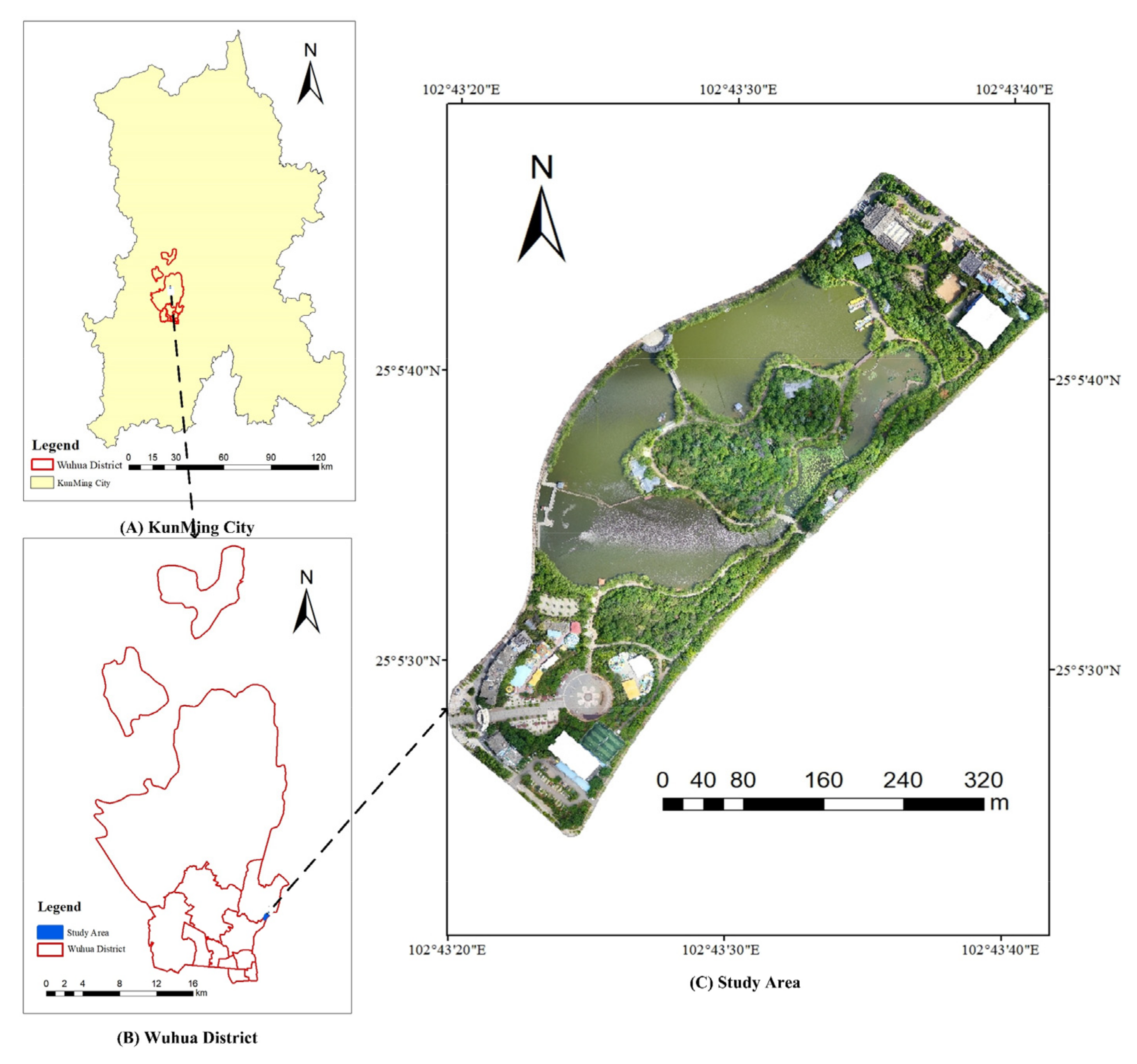
YueYaTan Park is a modern garden park with natural scenery, located in the northern sector of downtown Kunming, China (25°05′25″ N~25°05′45″ N, 102°43′22″ E~102°43′43″ E) (Figure 2). The park has two parts: the island in the center of the lake and the area outside the lake. It was built by the Wuhua District Government and was opened in October 2006. It has a coverage area of 160,000 m2. YueYaTan Park is located in a region with a subtropical highland monsoon climate, relatively high terrain, large amounts of sunshine, and sufficient rainfall, implying excellent plant growth. There are more than 60 plant species in park, and the greening rate is close to 60%, including the main vegetation species: Salix, Metasequoia, Sand jujube, and cinnamon, etc.

2.2. Data Acquisition

This study employed a four-rotor DJI phantom 4 RTK (SZ DJI Technology Co., Shenzhen, China) with an RGB digital camera to acquire high spatial-resolution imagery around YueYaTan Park on 29 April 2022. The UAV aerial photography system can obtain accurate GPS location information with a WGS-84 coordinate system and save it to images. The images have a resolution of 7952 × 5304 pixels in JPG format. The UAV was flown autonomously over the park at an altitude of 60 m, with a ground resolution of approximately 0.02 m, according to a predefined flight route programmed by the DJI ground station. To generate an orthophoto to cover the entire park, the main flight route direction was east–west, and the perpendicular direction was north–south with the forward and side overlap set to 80% and 70%, respectively. In addition, we assigned 12 ground control points (GCPs) to correct the spatial accuracy of the orthophotos. The mean RMS error was 0.024 m. The flight campaigns were conducted under clear skies and low wind speeds between 10:00 a.m. and 3:30 p.m. local time. Each flight duration was about 25 min to cover the study area. The ISO of the camera was set to 100, and the best exposure time of the camera was determined according to the weather conditions.
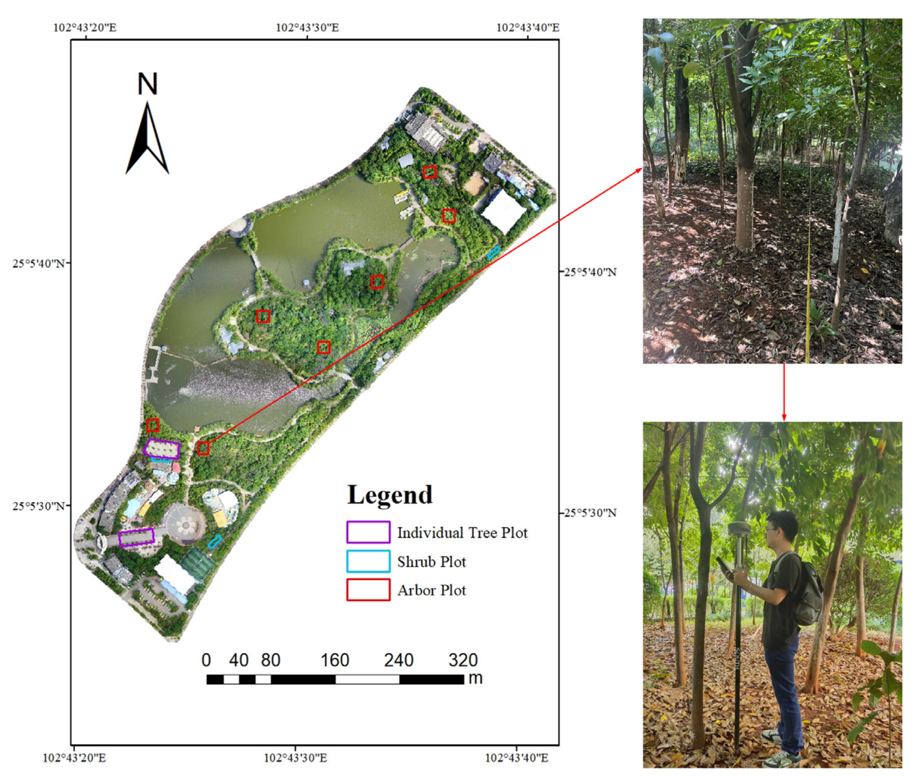
The field survey was conducted on 2 May 2022. A real-time kinematic instrument called ZHD V200 (RTK, GNSS, Guangzhou Hi-Target Navigation Tech Co., Ltd., Guangzhou, China) was used to determine the boundary of the sample plots and the coordinates of each individual tree. The sample plots are shown in Figure 3, and the details of the plots are listed in Table 2. Seven arbor plots were randomly located in the study area, with a size of 16 m × 16 m. Tree parameters, including crown height, crown diameter, first branch height, and crown shape of each tree, were measured, and the total number of trees was counted. In addition to the arbor plots, three shrub plots were positioned randomly, with an area of 256 m2, and average shrubs height was measured. Thirty-one individual trees were selected to avoid crown crossing and eliminate the influence of understory vegetation, such as roadside trees. A handheld digitalized and multi-functional forest measurement gun was used to measure tree and first branch height [41]. The average height of shrubs and crown diameters of each tree were measured with a tape measure. Two operators measured the crown diameter along the east–west and north–south directions. We measured all parameters three times and we used the mean value as the measured value.
The main tree species in the sample plots were Salix babylonica, Metasequoia glyptostroboides, Osmanthus fragrans, Elaeis guineensis, Elaeocarpus decipiens, Cinnamomum japonicum, Ficus microcarpa, Cycas revoluta. Based on these species, we summarized the “crown diameter–crown height” equations of the 3DGV estimation by other scholars’ studies (Table 3) [11,42] and used these equations to estimate the 3DGV for individual trees and each tree in sample plots. The equations were obtained from the crown volume equations. It has been proven that it is useful to simulate crown volume according to tree crown shapes using different regular volume formulas [43]. In the study of [42], the crown volume of was evaluated by measuring the volume using the sphere equation and had a relative bias of 16.4%. Another study [44] illustrated that crown volume calculated from geometrical formulas was feasible with an average relative RMSE of the flabellate formula of 12.5%. Liang et al. [45] compared the crown volume calculated from the ovoid equation and the measured value, which resulted in a relative error of between 7% and 10%. In addition, the crown volume of the cone equation deviated, on average, by 13.62% from the measured crown volume [46]. As for the shrub plots, due to the high density of shrubs, the 3DGV was calculated approximately by multiplying the area covered by shrubs by the height of the shrubs.

2.3. Vegetation Extraction

To improve the accuracy of the 3DGV, we first extracted the vegetated area of the study area before 3DGV estimation. According to a previous study [47], five vegetation indices (VIs) for visible wavelengths were used to extract the vegetated area based on RGB images using the Random Forest algorithm [48], including the Excess Green Index (ExG), Normalized Green-Red Difference Index (NGRDI), the construction of the Normalized Green-Blue Difference Index (NGBDI), the Red-Green Ratio (RGRI), and the Visible Band Difference Vegetation Index (VDVI). All equations for these vegetation indices are listed in Table 4.
The lack of NIR bands in UAV RGB images may lead to spectral fusion between vegetation and non-vegetation, which further results in poor extraction data when extracting the vegetation area. For solving this problem, texture features were also introduced to the extracted vegetation area. The texture features used in this study were textures derived from the gray-level co-occurrence matrix (GLCM), which determines the total co-occurrence of each pair of pixels in a given direction and at a certain distance in the image [49]. Fourteen correlated texture features were defined by Haralick [49]. We used six of the texture features with a gray level of 7, angle from 0° to 135°, distance of 1, and window size of 7 × 7 to extract the vegetated area in our study. This has been proven to improve the accuracy of vegetation extraction [50]. The six texture features (Table 5) were the mean (MEA), standard deviation (STD), homogeneity (HOM), dissimilarity (DIS), entropy (ENT), and angular second moment (ASM). In addition, considering the need to reduce the computational burden and that the Green band has a much higher importance than the Red or Blue bands because vegetation generally manifests green color, only the Green band was used for texture calculation [28].
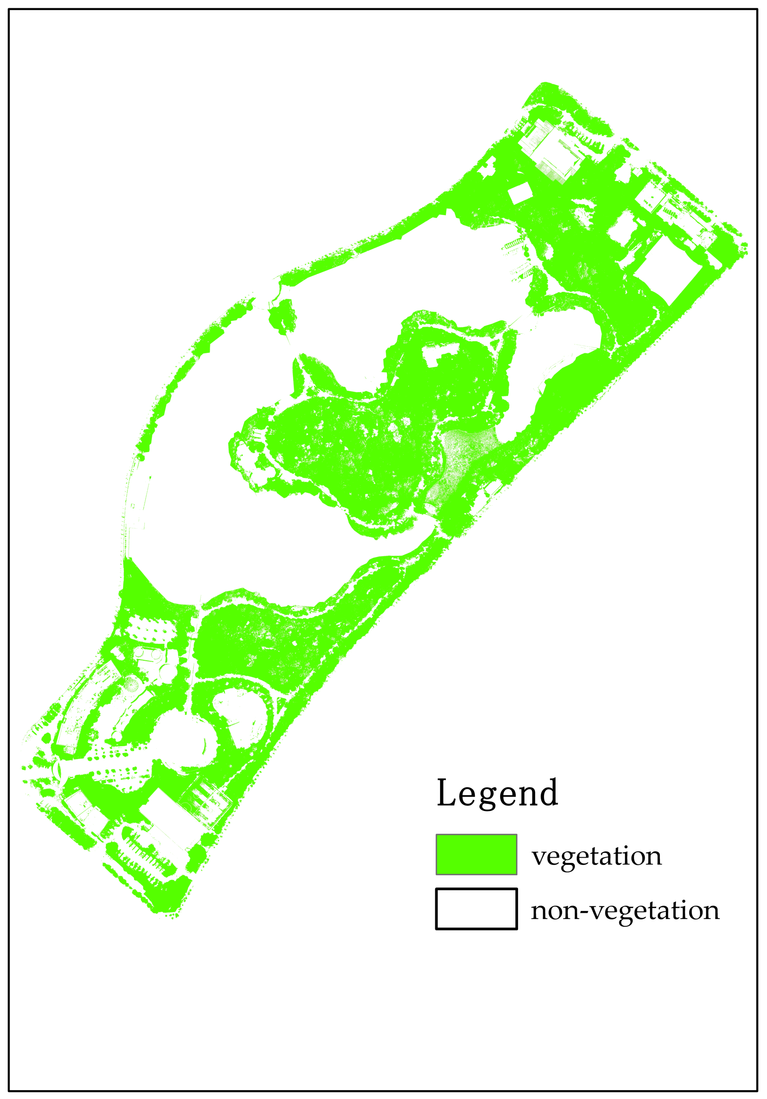
The Random Forest (RF) algorithm was used for vegetation and non-vegetation classification, which has been used frequently in recent years for image classification in remote sensing. RF is a machine learning method proposed in 2001 [48]. It has the advantages of not requiring variables to follow a specific statistical distribution, can be trained on small training samples, is less sensitive to overfitting, and has the ability to rank the importance of features for urban tree species’ classification. These advantages provide significant potential for classifying complex and texture-abundant UAV images. It has been widely applied to urban tree species’ classification [51,52]. The RF decision tree number in this study was set to 200, and the number of features each node used was the default value, which was the square root of the total number of features. The above-mentioned vegetation indices for visible wavelengths and texture features were incorporated into the RF classifier. The vegetation distribution after classification is shown in Figure 4.
A total of 2361 sample pixels were created randomly for classification into two types: vegetation and non-vegetation. One thousand, six hundred and fifty-three pixels served as training data and seven hundred and eight pixels were selected as validation data. The pixel-based confusion matrix was employed to describe accuracy, and the accuracy was evaluated by three accuracy evaluation metrics—producer accuracy (PA) user accuracy (UA), overall accuracy (OA)—and the Kappa coefficient. The confusion matrix and accuracy are listed in Table 6. The assessment results showed that our vegetation classification had reasonably high accuracy. The overall accuracy (OA) was 98.64% and with a Kappa coefficient of 0.98. The vegetation area had a producer accuracy (PA) of 98.24% and a user accuracy (UA) of 98.63%. The accuracy of our vegetation classification was close to previous studies [28,47], and it indicated that it is possible to estimate 3DGV with this vegetated map.

2.4. Estimation of 3DGV Based on the MNP Algorithm

We proposed a new method for estimation by combining the vegetation coverage and the canopy height in the specific cells. A large fishnet with a size of the integer multiple of the UAV RGB image resolution (0.02 m) was created on the orthophoto of the study area to determine the boundary of each specific gird. Then, the canopy height and vegetation coverage of each cell were calculated by the Canopy Height Model (CHM). The 3DGV of study area was estimated using the following equation:
G = i j S i × H i × C i
where G is the total 3DGV of the study area, i is the number of cells, j is the total number of cells. S i , H i , C i represent the area, canopy height, and vegetation coverage of each cell, respectively. For convenient calculation, we used a cell that size was 1.6 m × 1.6 m to estimate the 3DGV, which was one percent of the size of the arbor plots. The area of each cell was 2.56 m2.
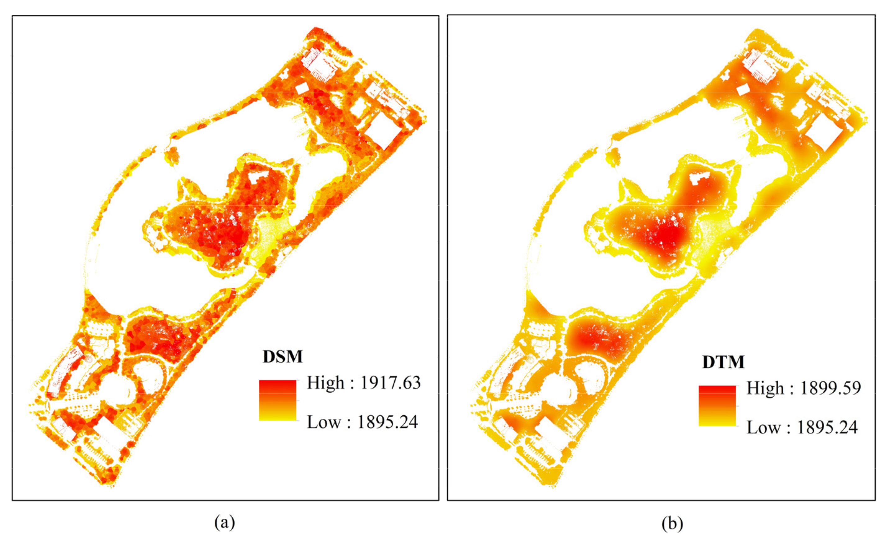
The CHM was constructed using the difference value between the Digital Surface Model (DSM) and Digital Terrain Model (DTM). First, the UAV image was decoded in an analytical aerial triangulation to produce high-density three-dimensional point cloud data. Second, the ground control points were used as the geographic location correction of the DSM, based on the point cloud data, and the point cloud data with obvious anomalies were manually cleared through visual interpretation. The median was 11,940.9 matches per calibrated image, and the average surface density of point cloud was 61.87/m2. Then, the DSM was built automatically on a Pix4D desktop and the DTM was generated by filtering out height information of the DSM, including buildings and vegetation. Finally, Gaussian filtering was employed to smooth the DSM to reduce image noise and improve the elevation of the vertices. The canopy height of each cell was the mean value of the CHM in each cell. The generated DSM and DTM are shown in Figure 5a,b, and the equation is as follow:
H i = D S M i D T M i
where H i is the average CHM of each cell, D S M i and D T M i are the average DSM and DTM of each cell, respectively.
The vegetation coverage was calculated on the vegetation distribution map from the percentage of vegetation pixels in the total pixels of each cell. The equation for the vegetation coverage is as follows:
C i = N n v N n t
where C i is the vegetation coverage of each cell, N n v is the number of vegetation pixels in each cell, and N n t is the total number of pixels in each cell.

2.5. Estimation of 3DGV Based on Tree Detection

2.5.1. Semi Variance Local Maximum Filtering

To demonstrate the method proposed in this paper was feasible, the traditional method of estimating 3DGV based on tree detection was used. Semi variance local maximum filtering was employed to detect trees. Digital images’ semi variance indicated pixel self-similarity over a transect of pixels. It provided a means of measuring the spatial dependency of a continuously varying phenomena [53]. The semi variance was calculated as follows:
γ h = 1 2 m h i = 1 m h Z x i Z x i h 2
where γ h is the semi variance, Z denotes the pixel value at a location x (where [ x = 1 ,   2 ,   3 ,   ,   n ]), the lag h indicates the distance between pairs for comparison. In each transect of values there will be m h observational pairs separated by the same lag distance h . If there is spatial structure in a given dataset, a semi variogram will reveal that semi variance rises until reaching a sill, which indicated the maximum variability between pixels. The pixels in this range imply the pixels related to the first pixel.
In this study, we first operated a moving window on the CHM to find the maximum value in every window. The size of the moving window was the smallest crown diameter of measured field data. Each pixel of the maximum value was considered to be the potential vertex of a tree. Then, we calculated the semi variance in eight cardinal directions of every potential vertex and determined lag distances h 1 ~ 8 . All pixels on h created the potential ranges of each potential vertex. By comparing the CHM value of all potential vertex in each potential range, the potential vertex of the maximum value in each potential range was considered compared to the detected vertex of a tree. The maximum allowable lag location was set as the radius of the biggest tree crown in study area, which was 200 pixels, and 4 m.

2.5.2. Segmentation by Mean Shift Algorithm

Prior to estimating 3DGV, the tree crown must be defined. Based on the detected vertex of each tree, the mean shift algorithm was employed to extract the tree crown and finish the segmentation. The mean shift algorithm is a simple iterative process that shifts each data point to the center point in its neighborhood by computing the offset mean value. The neighborhood was determined to be a cluster [54]. The offset mean value was calculated as follows:
M x = 1 k x i S h x x i
where M x is the offset mean value, S h is a high dimensional sphere with radius h and center x , x i is the sample point, k indicates the number of points falling into the S(h) in x i , x x i is the offset vector of x .
This algorithm was implemented in five steps as follows: Step 1: Initialize all detected vertex as the first center point and describe all pixels in the ranges of the detected vertex with a set named M. Step 2: Compute the offset vectors of each center point to all pixels in M and add all offset vectors and calculate the mean value. Step 3: Move the center point in the direction of the offset vector and the distance is the norm of the offset vector. Step 4: Set a threshold based on the size of the smallest tree crown, iterate step 2, step 3, and record the center point when the offset mean value reaches the threshold. Step 5: Iterate the above steps until all pixels are classified to a cluster.

2.5.3. Estimation of 3DGV Based on the Convex Hull Algorithm

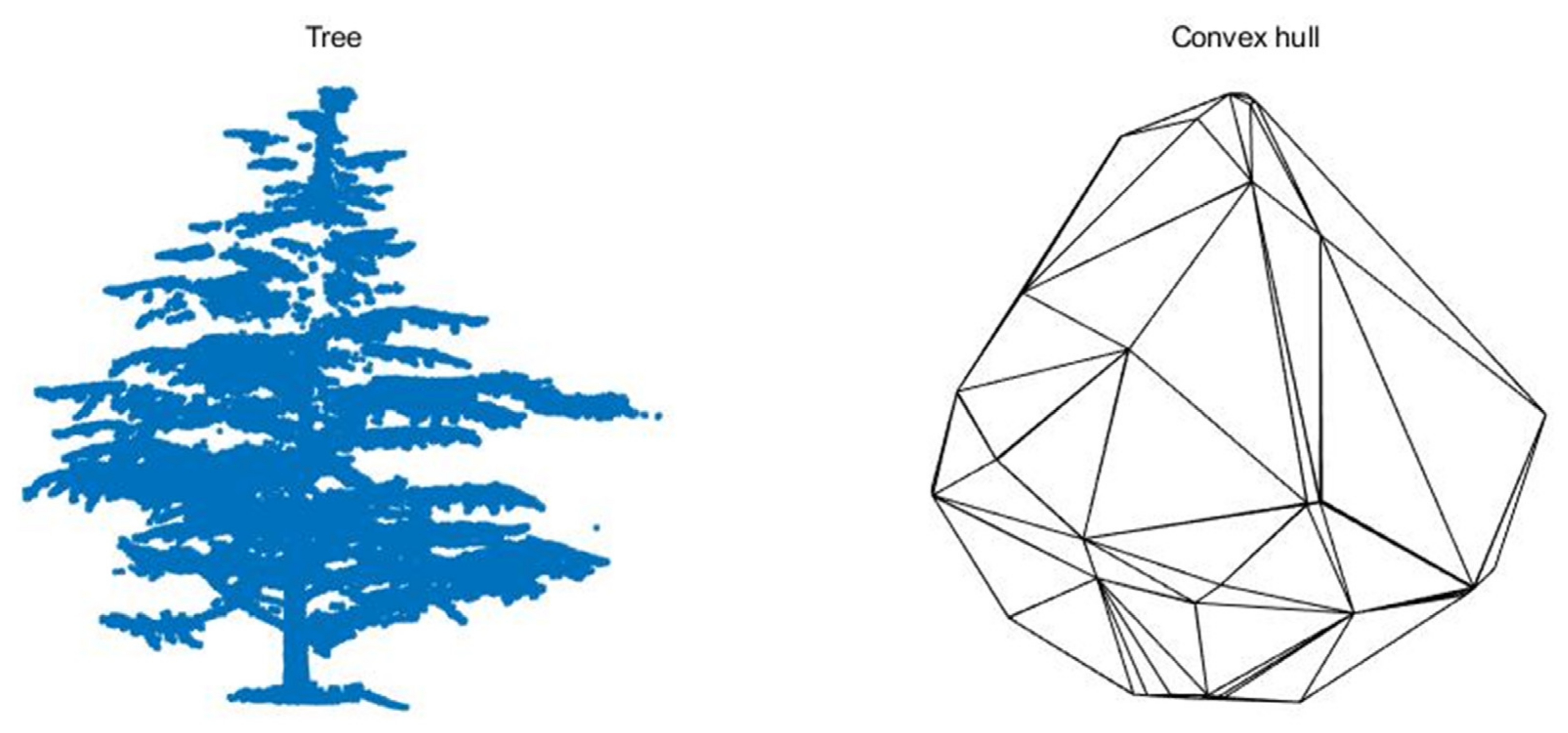
The Convex hull algorithm estimates 3DGV based on the crown volume. It no longer calculates crown volume as a regular geometry but simulates the irregular three-dimensional shape of the crown by a convex polyhedron. We defined the pixels of each tree crown to the x-y coordinates and created a three-dimensional coordinate system with the CHM value of each tree crown as the z coordinate. All pixels were connected to each other with the coordinates, which made multi-polygons, according to different connection orders [18]. The Convex hull function in MATLAB was used to find the maximum polyhedron and calculated volume of polyhedrons as the 3DGV of trees. The algorithm diagram is shown in Figure 6.

2.5.4. Estimation of 3DGV Based on the Voxel Algorithm

The Voxel model is composed of individual cubic elements. A voxel is the 3-D counterpart of a pixel in an image and relates to an elementary volume, typically having a square base. We determined the tree crown composed of voxel models, and the 3DGV was estimated by the sum of the crown voxel volume [55]. The 3DGV based on the Voxel algorithm was calculated as follow:
G v s , t = i = 1 s j = 1 t d 2 × H i j
where G v s , t is the 3DGV of each tree crown, s and t are the numbers of rows and columns in pixels of the image, d 2 is the resolution of the images, i and j are the number of individual cubic elements, H i j is the CHM value of current voxel. The sum of all G v is the 3DGV of study area.

2.6. Accuracy Assessment

The results of the computation in this study were evaluated using the measured value of the field survey. The tree and canopy heights were used to evaluate the CHM, and the 3DGV computed in field survey was used to evaluate the 3DGV estimated based on three algorithms. The arbor and shrub plots were both used as evaluation plots. Three accuracy assessment metrics—bias, coefficient of determination (R2), and root mean square error (RMSE)—were employed to evaluate the performance of the algorithms. The equations for accuracy assessment that we used are defined as follows:
B i a s = i = 1 n y i y r i   n
R M S E = i = 1 n y i y r i 2 n 1
R 2 = 1 i = 1 n y r i   y i 2 i = 1 n y r i   y r ¯ 2
where y i is the estimated value, y r i is the reference value, y r ¯ is the mean value of the reference value, and n is the number of estimates. Relative bias and RMSE were also employed to evaluate the mapping result, which was calculated by dividing bias and RMSE by the mean of the reference values.

3. Results

3.1. The Canopy Height and Vegetation Coverage

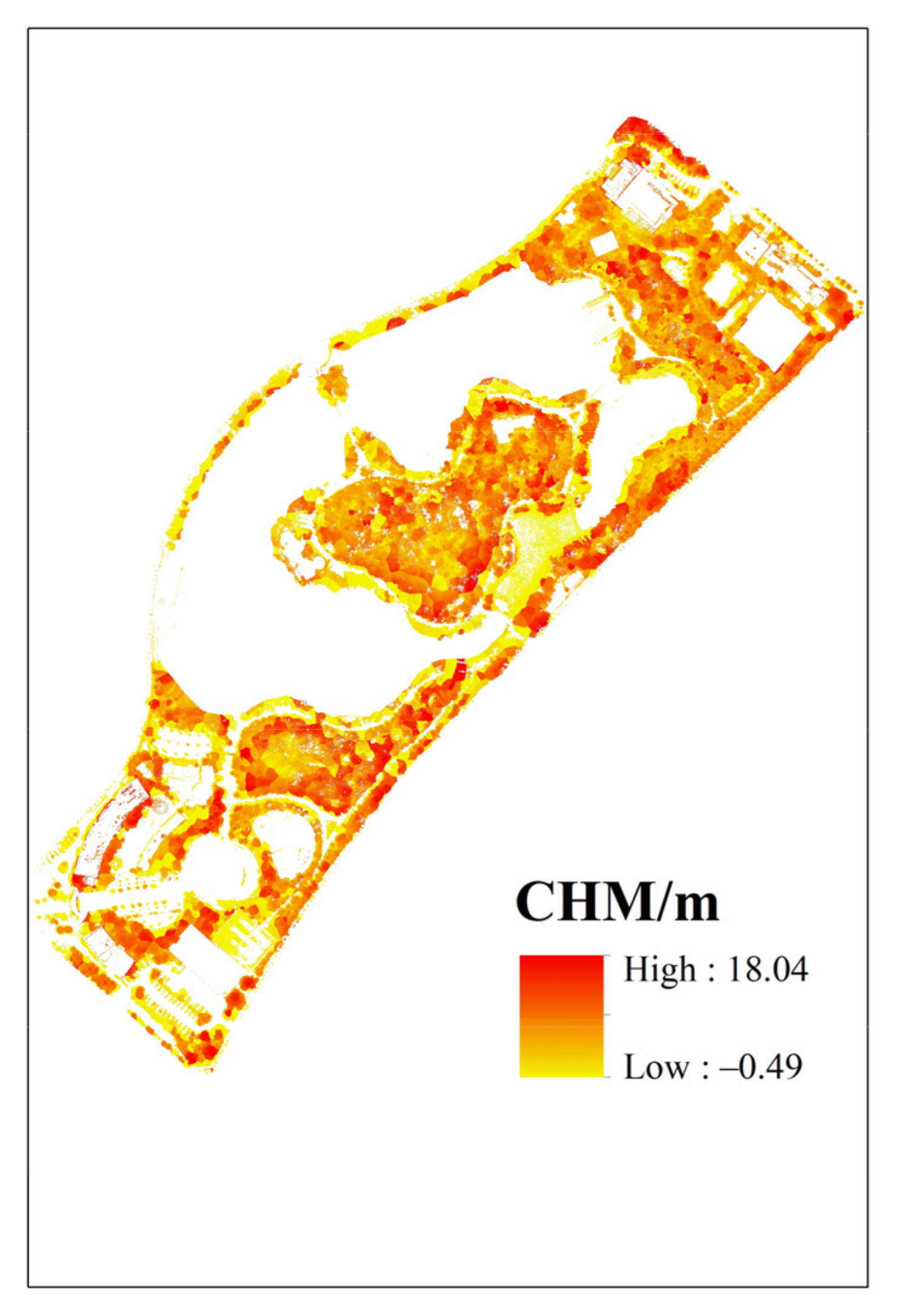
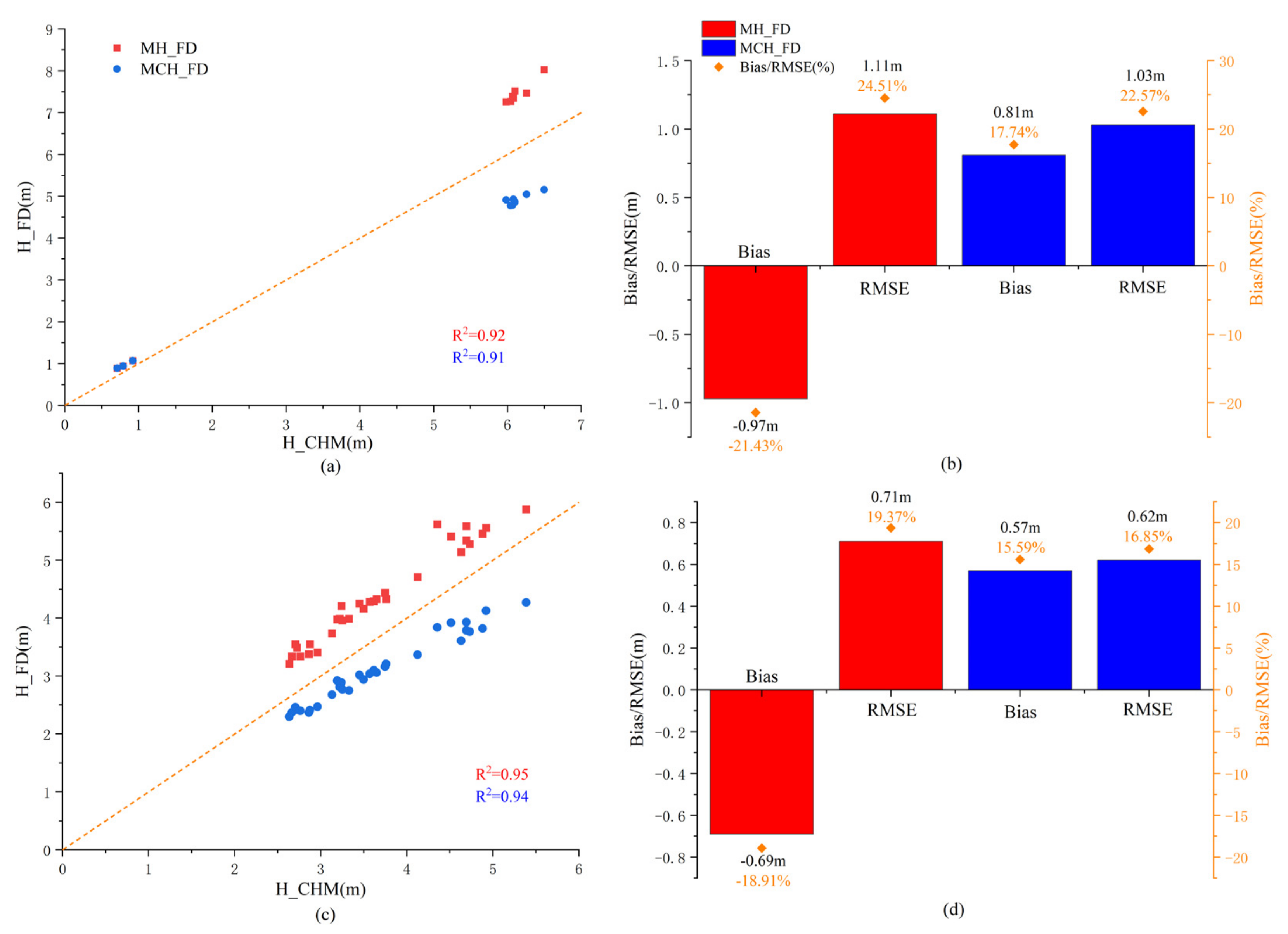
We compared the CHM map extracted using our method (Figure 7) against the tree height and canopy height of reference measurements (Figure 8). The canopy height in the vegetated area was higher on the island in the lake center and lower in the area outside the lake. In addition, some higher values were distributed in the east of study area (Figure 7). As illustrate in scatter plots, the coefficient of the determination R2 of the CHM against MH_FD was 0.92 for plots and 0.95 for individual trees, and R2 of the CHM against MCH_FD was 0.91 for pots and 0.94 for individual trees (Figure 8a). These values of R2 indicated that the CHM had a high correlation with the measured field data, which proved the feasibility of the CHM. On the other hand, the Bias of MCH_FD was 0.81 m (17.74%) and the RMSE of MCH_FD was 1.03 m (22.57%) for plots. The Bias of MCH_FD was 0.57 m (−15.59%) and the RMSE of MCH_FD was 0.62 m (16.85%) for individual trees (Figure 8b). It is worth noting that the deviation between the CHM and MCH_FD for plots and individual trees was positive, which explains that the canopy heights determined from the CHM were overestimated by the field data and resulted in more errors in plots.
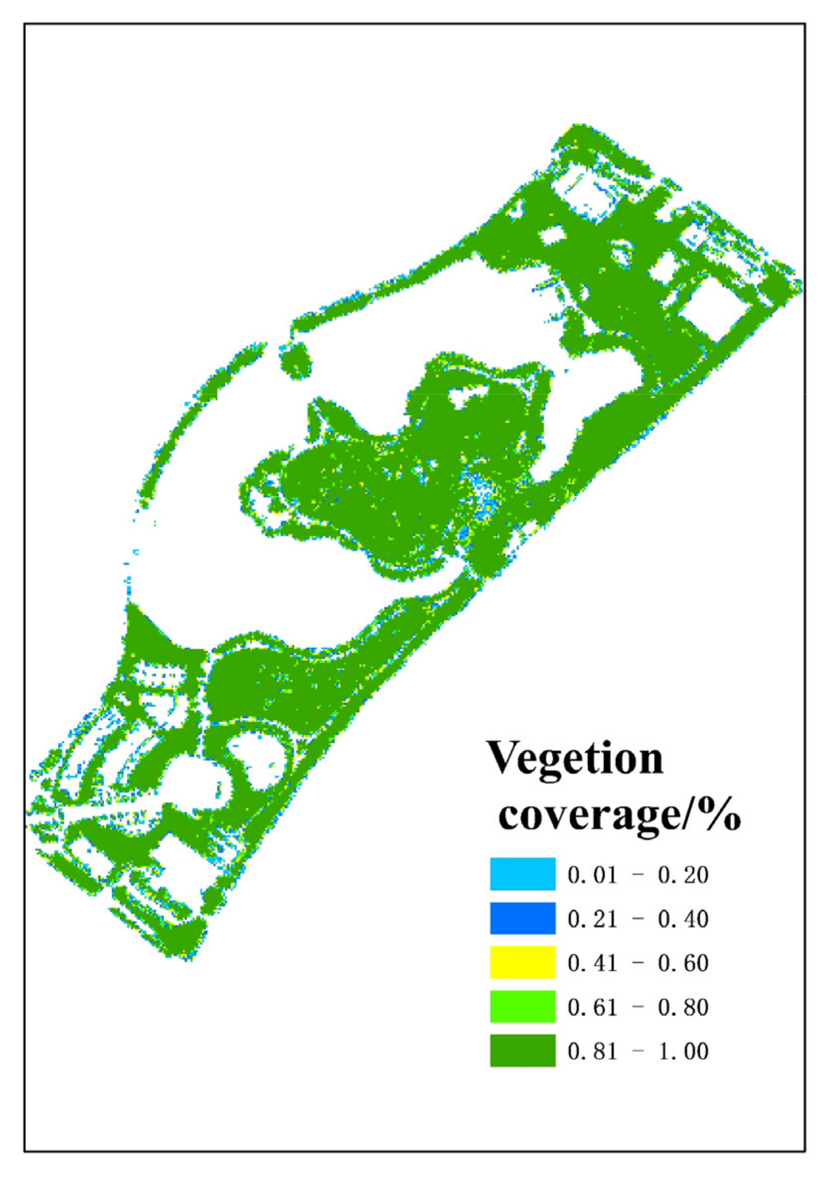
The vegetation coverage in the entire study area was relatively consistent. The coverage of most vegetated areas was high. A lower coverage area only occurred in the distribution of individual trees and at the edge of the vegetated area (Figure 9).

3.2. Accuracy Assessment of 3DGV

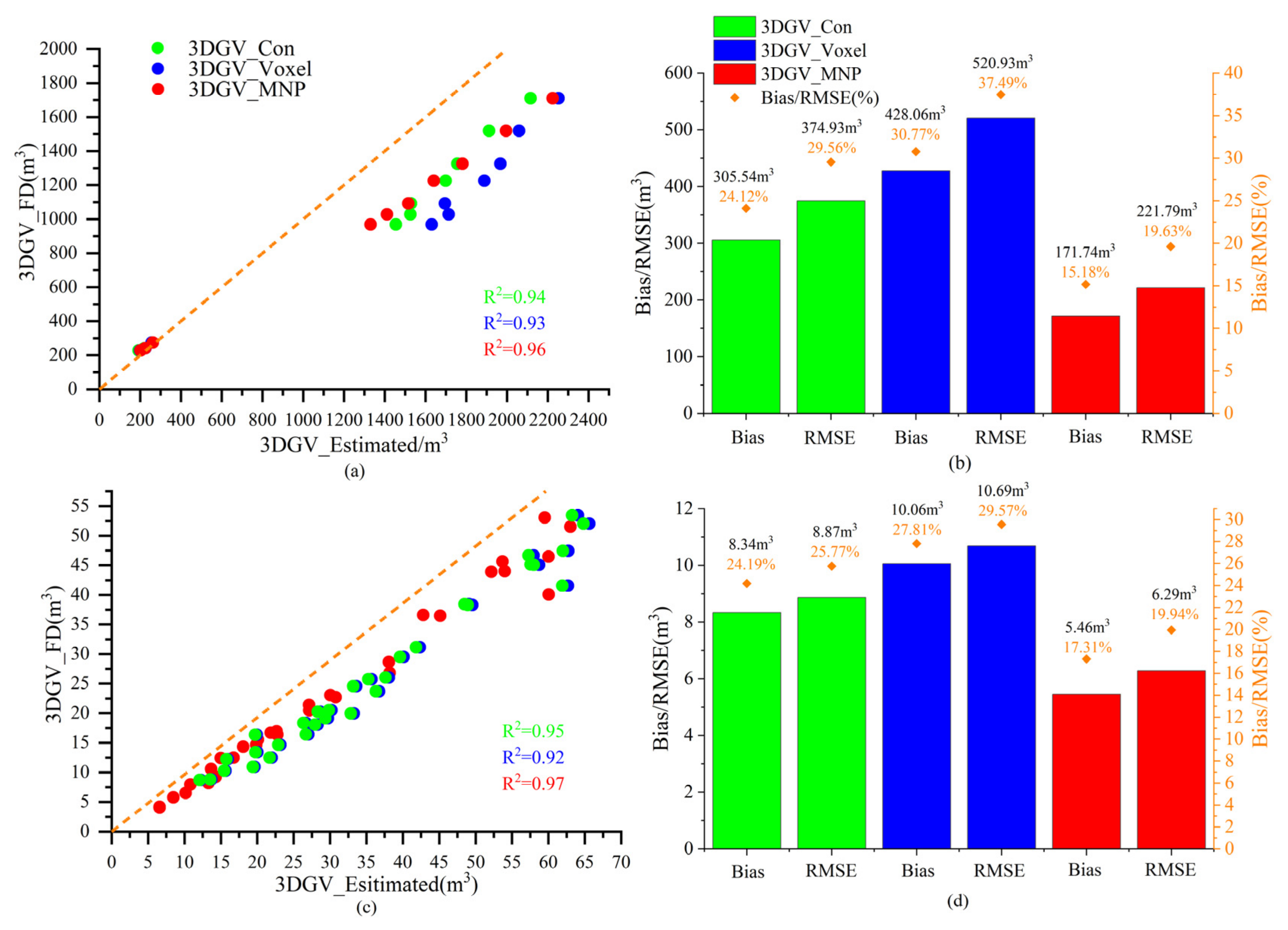
To evaluate the performance of the proposed approach, we compared the 3DGV_FD with 3DGV_Con, 3DGV_Voxel, and 3DGV_MNP (Figure 10). As described in scatter diagrams, the correlation analysis revealed that the R2 value of three algorithms was 0.94, 0.93, 0.96 for plots, respectively, and 0.95, 0.92, and 0.97 for individual trees, respectively (Figure 10a,c). The results of the correlation analysis indicated that all three algorithms can be used to estimate 3DGV, but the MNP algorithm performs slightly better than the others. Furthermore, we compared the performance of 3DGV_Con, 3DGV_Voxel, and 3DGV_MNP with 3DGV_FD (Figure 10b,d). The results showed that the Bias and RMSE of 3DGV_MNP was 171.74 m3 (15.18%) and 227.79 m3 (19.63%) for plots, and 5.46 m3 (17.31%) and 6.29 m3 (19.94%) for individual trees, respectively. The deviation between 3DGV_MNP and 3DGV_FD demonstrated the feasibility of estimating 3DGV based on UAV RGB images at the pixel level. In addition, the Bias and RMSE of 3DGV_Con were 305.54 m3 (24.12%) and 374.93 m3 (24.56%) for plots, and 8.34 m3 (24.19%) and 8.87 m3 (25.77%) for individual trees, respectively. However, 3DGV_Con was larger than 3DGV_MNP but smaller than 3DGV_Voxel. The Bias and RMSE of 3DGV_Voxel were 428.06 m3 (30.77%) and 520.93 m3 (37.49%) for plots, and 10.06 m3 (27.81%) and 10.69 m3 (29.57%) for individual trees, respectively. In conclusion, although all algorithms overestimated the 3DGV values when compared to field data, the MNP algorithm exhibited better performance than the others, indicating that estimating 3DGV based on pixels is superior to estimating based on tree detection. The overestimation may be attributed to the CHM, which was found to overestimate the canopy height. Moreover, the tree detection method introduced errors in areas with high vegetation density and coverage, explaining why the MNP algorithm outperformed the Convex hull and Voxel algorithms.

3.3. The Maps of 3DGV

Overall, the total 3DGV_MNP of YueYaTan Park was 377,223.21 m3. The 3DGV spatial distribution indicated that the 3DGV values fluctuated within a certain range, and the overall trend was consistent with the spatial distribution pattern (Figure 11a). The 3DGV spatial distribution also showed that there were differences in the 3DGV values among different transects, which may be related to the distribution of tree species, vegetation coverage, and soil conditions. These results suggested that the proposed method can effectively estimate the 3DGV of UGS and provide valuable information for the management and planning of UGS.
In order to compare the results of 3DGV_Con and 3DGV_Voxel with 3DGV_MNP, the former two were normalized to the same size as the cell of 3DGV_MNP (Figure 11b,c). The total 3DGV_Con and 3DGV_Voxel was 416,472.33 m3 and 442,795.64 m3, respectively. The results demonstrated that 3DGV_MNP was the smallest, while 3DGV_Voxel was the largest in the study area. This further supports the notion that the estimation of 3DGV based on pixels is smaller than based on tree detection. These findings also indicated that the algorithms of tree detection can overestimate the 3DGV, and the errors increased with increasing tree numbers. Additionally, it was observed that 3DGV_Con was smaller than 3DGV_Voxel, which could be due to the geometry models obtained by the Convex hull algorithm being closer to the trees than voxel models.

4. Discussion

4.1. The Process of Tree Detection

As illustrated in the results of Section 3.3, we considered the reason for why the Bias and RMSE of estimation based on tree detection were smaller than the estimation based on the MNP algorithm in UGS. The details of the tree detection are shown in Figure 12 shows that from the detected vertices on the orthophoto and results of segmentation, it is obvious that most of the tree vertices in the plots can be accurately marked, especially for individual trees. However, in the vegetation areas with a flat crown or dense crown, the detected vertices were marked on the same tree or some trees were omitted whose CHM was close to neighboring trees. The segmentation algorithm applied in these detected vertices caused errors in number of trees. Some neighboring trees were segmented to one tree, including the gaps between trees, which implies that it could cause overestimation in the 3DGV estimation. This phenomenon indicated that detecting trees by CHM to estimate 3DGV is not the best choice in vegetated areas with complex vegetation distribution, and the vegetation distribution in UGS is most complex.

4.2. Innovations and Limitations

Many previous studies have been carried out in the pursuit of 3DGV estimation. Compared with them, our method has some innovations. First, we found the UAV with RGB sensors can be employed for 3DGV estimation. It is more suitable for investigation in UGS because of its low cost and high efficiency, which can replace LIDAR scanning technology. Second, we proved 3DGV estimation can be achieved via pixels and also enables 3DGV estimation with completeness and correctness levels on par with other approach. For example, a study using backpack laser scanning to estimate 3DGV by crown height and diameter had an average relative error of 20.9% compared to the measured data [18]. Another study constructed the estimation model of 3DGV in an urban forest established on high-precision 3D laser-scanned point cloud data had a high estimation user accuracy of 88.07% [56]. In our study, we used the MNP algorithm to estimate 3DGV and compared it with the measurement reference, which achieved a bias of 15.18% for plots and 17.31% for individual trees. Third, we demonstrated that the MNP algorithm performed better in UGS by comparing it with two algorithms based on tree detection. The complex distribution of vegetation and the gaps between plants were both considered in our algorithm, which are limitations of other algorithms.
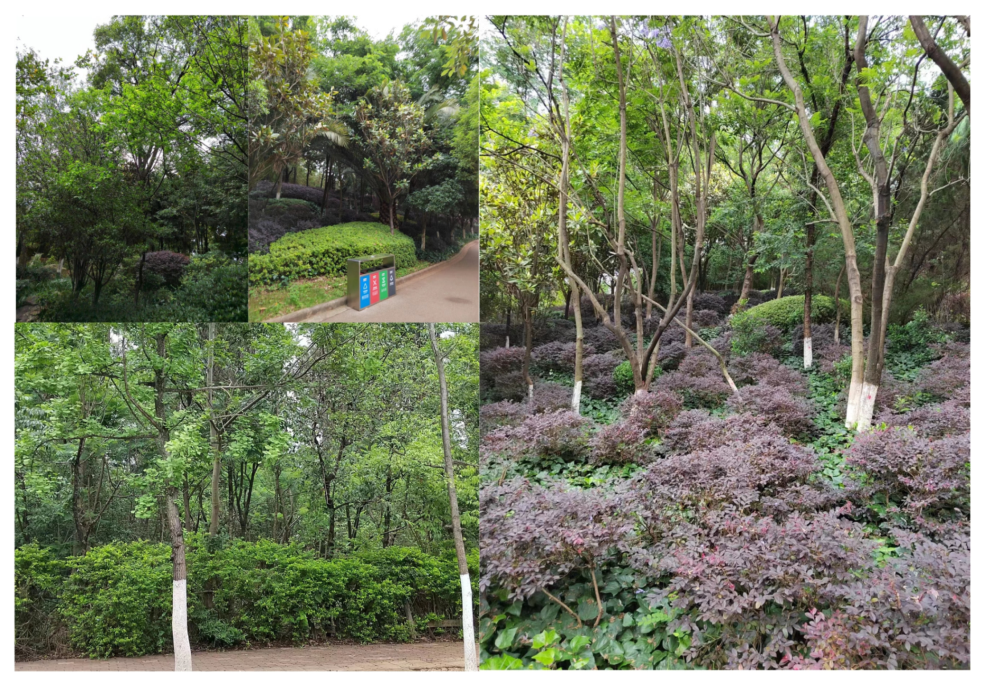
Although the MNP algorithm we used in this study performed well, there are certain limitations. First, the tree height obtained based on the deviation of the DSM and DTM was underestimated compared to field data. There are a few possible reasons for this underestimation. One reason is human error. The tree density in the plots was too high to measure tree height accurately in the field survey. Another reason may be device error. The UAV point cloud data are inaccurate due to small ground points and the automatic generation by Pix4D may result in an error in the DSM and DTM. For example, Bai et al. [57] used Pix4D to preprocess UAV images of UGS and generated the CHM by the difference between the DSM and DTM, which had an R2 of 0.89 and relative RMSE of 87.58% compared to the field measured data. Another study [58] also used Pix4D to process UAV LIDAR point cloud data of spruce plots, and obtain the CHM, which produced an RMSE of 1.39 m compared to the measured canopy height. The above results are consistent with our research and provide a reference for the tree height underestimation. Second, there were some shadows on the orthophoto due to the time difference between the UAV flight and the sun altitude angle when extracting the vegetated area. Unfortunately, we did not find a satisfactory method to eliminate the shadows on the RGB images, and they may have caused errors in vegetation extraction. Third, several previous studies based on point cloud data have underestimated the 3DGV of individual trees compared to the results of “crown diameter–crown height” equations [18,19,59]. These studies considered the gaps between the tree crowns, and their results were closer to the real 3DGV. However, the 3DGV_MNP of the individual trees was overestimated compared to the results of “crown diameter–crown height” equations. Therefore, the total 3DGV_MNP of the study area may be much larger than the real 3DGV. Fourth, it is important to note that in the case of UAV data, only the canopy surfaces were captured, and thus the volume of stem and lower parts of the canopy have not been accurately calculated. Unfortunately, we were not able to obtain the information of these parts. For individual trees, the volume of these parts was significantly small and only occupied a small part of the 3DGV of the study area. For areas with a high vegetation density, there were many plants growing under the canopy (Figure 13). The 3DGV of these plants was calculated by the MNP algorithm, and we considered that this was the volume the 3DGV below the canopy. However, the inability to accurately obtain the 3DGV of the stem and lower parts of the canopy remains an issue in this study. In future studies, we will further improve the above limitations and conduct more in-depth research to enhance the accuracy of the 3DGV.

5. Conclusions

3DGV is a three-dimensional index that accurately reflects vegetation configuration and the extent of UGS. As a method to assess urban greening and urban ecology, 3DGV becomes an increasingly important factor. In this study, we used a new method to estimate 3DGV and applied it to high-resolution aerial survey images of YueYaTan Park in Kunming City. We extracted the vegetated area, built a CHM, calculated the vegetation coverage, and estimated the 3DGV based on the Mean of neighboring pixels (MNP) algorithm. Then, the 3DGV was compare to 3DGV_MNP, based on tree detection with two algorithms, the Convex hull algorithm and Voxel algorithm, and the accuracy of the results based on field data was assessed. Our results indicated the performance of the MNP algorithm is better than the two algorithms in tree detection. The deviation of 3DGV_MNP for individual trees (Relative Bias = 17.31%, Relative RMSE = 19.94%, R2 = 0.95) and for plots (Relative Bias = 15.18%, Relative RMSE = 19.63%, R2 = 0.96) were both suitable for 3DGV estimation in UGS. The results of 3DGV_MNP showed that the total 3DGV was 377,223.21 m3 in YueYaTan Park. It is concluded that 3DGV estimation can be realized without obtaining the parameters of each tree, and the MNP algorithm is better than tree detection for estimating 3DGV in UGS with a complex vegetation distribution. Our study proposed a rapid and effective method for 3DGV estimation on UAV RGB images. It can save time when extracting and calculating individual tree parameters, solve previous problems of being unable to completely extract vegetated strains from UAV remote sensing images in high-density vegetated areas, and improve the efficiency and accuracy of 3DGV estimations. This study can provide technical support for the accurate quantitative evaluation of the ecological benefits of UGS.

Author Contributions

W.X. and Z.H. designed the study. W.X., Z.H., and Y.L. conducted the data analyses. L.W. and N.L. contributed to the algorithm. W.X., Z.H., and Q.D. wrote the draft manuscript, G.O. contributed to the manuscript revision, and all the authors contributed to the interpretation of results and manuscript writing. All authors have read and agreed to the published version of the manuscript.

Funding

This research was supported in part by research grants from the National Natural Science Foundation of China (grant number 32060320, 32160369, 32160368); Research Foundation for Basic Research of Yunnan Province (grant number 202101AT070039); “Ten Thousand Talents Program” Special Project for Young Top-notch Talents of Yunnan Province (grant number YNWR-QNBJ-2020047); Joint Special Project for Agriculture of Yunnan Province, China (grant number 202101BD070001-066); The Key Development and Promotion Project of Yunnan Province under Grant (grant number 202102AE090051).

Acknowledgments

We thank the XZB Technology Company for their UAV devices and data. We thank the anonymous reviewers for their constructive comments on the earlier version of the manuscript.

Conflicts of Interest

The author declare no conflict of interest.

References

  1. Xiong, Y.; Zhao, S.; Yan, C.; Qiu, G.; Sun, H.; Wang, Y.; Qin, L. A comparative study of methods for monitoring and assessing urban green space resources at multiple scales. Remote Sens. Land Resour. 2021, 33, 54–62. [Google Scholar]
  2. Kondo, M.C.; Fluehr, J.M.; McKeon, T.; Branas, C.C. Urban green space and its impact on human health. Int. J. Environ. Res. Public Health 2018, 15, 445. [Google Scholar] [CrossRef] [PubMed] [Green Version]
  3. Nath, T.K.; Han, S.S.Z.; Lechner, A.M. Urban green space and well-being in Kuala Lumpur, Malaysia. Urban For. Urban Green. 2018, 36, 34–41. [Google Scholar] [CrossRef]
  4. Bertram, C.; Rehdanz, K. The role of urban green space for human well-being. Ecol. Econ. 2015, 120, 139–152. [Google Scholar] [CrossRef] [Green Version]
  5. Richardson, E.A.; Pearce, J.; Mitchell, R.; Kingham, S. Role of physical activity in the relationship between urban green space and health. Public Health 2013, 127, 318–324. [Google Scholar] [CrossRef] [PubMed] [Green Version]
  6. Wolch, J.R.; Byrne, J.; Newell, J.P. Urban green space, public health, and environmental justice: The challenge of making cities ‘just green enough’. Landsc. Urban Plan. 2014, 125, 234–244. [Google Scholar] [CrossRef] [Green Version]
  7. Dobbs, C.; Kendal, D.; Nitschke, C. The effects of land tenure and land use on the urban forest structure and composition of Melbourne. Urban For. Urban Green. 2013, 12, 417–425. [Google Scholar] [CrossRef]
  8. Kendal, D.; Williams, N.S.G.; Williams, K.J.H. Drivers of diversity and tree cover in gardens, parks and streetscapes in an Australian city. Urban For. Urban Green. 2012, 11, 257–265. [Google Scholar] [CrossRef]
  9. Chen, Z. Research on the ecological benefits of urban landscaping in Beijing (2). China Gard. 1998, 14, 51–54. [Google Scholar]
  10. Zhou, J.H. Research on the green quantity group of urban living environment (5)—Research on greening 3D volume and its application. China Gard. 1998, 14, 61–63. [Google Scholar]
  11. Zhou, T.; Luo, H.; Guo, D. Remote sensing image based quantitative study on urban spatial 3D Green Quantity Virescence three dimension quantity. Acta Ecol. Sin. 2005, 25, 415–420. [Google Scholar]
  12. Alonzo, M.; Bookhagen, B.; Roberts, D.A. Urban tree species mapping using hyperspectral and lidar data fusion. Remote Sens. Environ. 2014, 148, 70–83. [Google Scholar] [CrossRef]
  13. Calders, K.; Adams, J.; Armston, J.; Bartholomeus, H.; Bauwens, S.; Bentley, L.P.; Chave, J.; Danson, F.M.; Demol, M.; Disney, M. Terrestrial laser scanning in forest ecology: Expanding the horizon. Remote Sens. Environ. 2020, 251, 112102. [Google Scholar] [CrossRef]
  14. Williams, J.; Schonlieb, C.-B.; Swinfield, T.; Lee, J.; Cai, X.; Qie, L.; Coomes, D.A. 3D Segmentation of Trees Through a Flexible Multiclass Graph Cut Algorithm. IEEE Trans. Geosci. Remote Sens. 2020, 58, 754–776. [Google Scholar] [CrossRef]
  15. Cheng, L.; Chen, S.; Chu, S.; Li, S.; Yuan, Y.; Wang, Y.; Li, M. LiDAR-based three-dimensional street landscape indices for urban habitability. Earth Sci. Inform. 2017, 10, 457–470. [Google Scholar] [CrossRef]
  16. He, C.; Convertino, M.; Feng, Z.; Zhang, S. Using LiDAR data to measure the 3D green biomass of Beijing urban forest in China. PLoS ONE 2013, 8, e75920. [Google Scholar] [CrossRef]
  17. Huang, Y.; Yu, B.; Zhou, J.; Hu, C.; Tan, W.; Hu, Z.; Wu, J. Toward automatic estimation of urban green volume using airborne LiDAR data and high resolution remote sensing images. Front. Earth Sci. 2013, 7, 43–54. [Google Scholar] [CrossRef]
  18. Li, X.; Tang, L.; Peng, W.; Chen, J. Estimation method of urban green space living vegetation volume based on backpack light detection and ranging. Chin. J. Appl. Ecol. 2021, 33, 2777–2784. [Google Scholar]
  19. Wang, J.; Yang, H.; Feng, Z. Tridimensional Green Biomass Measurement for Trees Using 3-D Laser Scanning. Trans. Chin. Soc. Agric. Mach. 2013, 44, 229–233. [Google Scholar]
  20. Cabo, C.; Del Pozo, S.; Rodríguez-Gonzálvez, P.; Ordóñez, C.; González-Aguilera, D. Comparing terrestrial laser scanning (TLS) and wearable laser scanning (WLS) for individual tree modeling at plot level. Remote Sens. 2018, 10, 540. [Google Scholar] [CrossRef] [Green Version]
  21. Huo, L.; Zhang, N.; Zhang, X.; Wu, Y. Tree defoliation classification based on point distribution features derived from single-scan terrestrial laser scanning data. Ecol. Indic. 2019, 103, 782–790. [Google Scholar] [CrossRef]
  22. Hyyppä, E.; Kukko, A.; Kaijaluoto, R.; White, J.C.; Wulder, M.A.; Pyörälä, J.; Liang, X.; Yu, X.; Wang, Y.; Kaartinen, H. Accurate derivation of stem curve and volume using backpack mobile laser scanning. ISPRS J. Photogramm. Remote Sens. 2020, 161, 246–262. [Google Scholar] [CrossRef]
  23. Liu, G.; Wang, J.; Dong, P.; Chen, Y.; Liu, Z. Estimating individual tree height and diameter at breast height (DBH) from terrestrial laser scanning (TLS) data at plot level. Forests 2018, 9, 398. [Google Scholar] [CrossRef] [Green Version]
  24. Sun, Y. A Estimation Model of Tridimensional Green Biosmass Established on GF-2 Remote Sensing Data. Master’s Thesis, University of Geosciences, Beijing, China, 2017. [Google Scholar]
  25. Wang, P. The Esimation of Living Vegetation Volume in the Ring Park around Hefei City Based on TLS and Landsat8. Master’s Thesis, Anhui Agricultural University, Hefei, China, 2018. [Google Scholar]
  26. Xie, L.; Zhang, X.; Song, J. Estimation for tridimensional green biomass based on TM remote sensing image. J. Nanjing For. Univ. (Nat. Sci. Ed.) 2015, 39, 104–108. [Google Scholar]
  27. Yi, Y.; Zhang, G.; Zhang, L. Research of 3D Green Quantity of Urban Vegetation Based on GF-2 Remote Sensing Image. Intell. Constr. Urban Green Space 2020, 2–7. [Google Scholar]
  28. Feng, Q.; Liu, J.; Gong, J. UAV Remote Sensing for Urban Vegetation Mapping Using Random Forest and Texture Analysis. Remote Sens. 2015, 7, 1074–1094. [Google Scholar] [CrossRef] [Green Version]
  29. Torres-Sánchez, J.; Peña, J.M.; de Castro, A.I.; López-Granados, F. Multi-temporal mapping of the vegetation fraction in early-season wheat fields using images from UAV. Comput. Electron. Agric. 2014, 103, 104–113. [Google Scholar] [CrossRef]
  30. Xu, E.; Guo, Y.; Chen, E.; Li, Z.; Zhao, L.; Liu, Q. Deep learning remote sensing estimation method (UnetR) for regional forest canopy closure combined with UAV LiDAR and high spatial resolution satellite remote sensing data. Geomat. Inf. Sci. Wuhan Univ. 2021, 47, 1298–1308. [Google Scholar]
  31. Wallace, L.; Lucieer, A.; Watson, C.; Turner, D. Development of a UAV-LiDAR system with application to forest inventory. Remote Sens. 2012, 4, 1519–1543. [Google Scholar] [CrossRef] [Green Version]
  32. Xu, W.; Deng, S.; Liang, D.; Cheng, X. A crown morphology-based approach to individual tree detection in subtropical mixed broadleaf urban forests using UAV LiDAR data. Remote Sens. 2021, 13, 1278. [Google Scholar] [CrossRef]
  33. Zhou, L.; Meng, R.; Tan, Y.; Lv, Z.; Zhao, Y.; Xu, B.; Zhao, F. Comparison of UAV-based LiDAR and digital aerial photogrammetry for measuring crown-level canopy height in the urban environment. Urban For. Urban Green. 2022, 69, 127489. [Google Scholar] [CrossRef]
  34. Ge, H.; Xiang, H.; Ma, F.; Li, Z.; Qiu, Z.; Tan, Z.; Du, C. Estimating plant nitrogen concentration of rice through fusing vegetation indices and color moments derived from UAV-RGB images. Remote Sens. 2021, 13, 1620. [Google Scholar] [CrossRef]
  35. Li, L.; Chen, J.; Mu, X.; Li, W.; Yan, G.; Xie, D.; Zhang, W. Quantifying understory and overstory vegetation cover using UAV-based RGB imagery in forest plantation. Remote Sens. 2020, 12, 298. [Google Scholar] [CrossRef] [Green Version]
  36. Liang, Y.; Kou, W.; Lai, H.; Wang, J.; Wang, Q.; Xu, W.; Wang, H.; Lu, N. Improved estimation of aboveground biomass in rubber plantations by fusing spectral and textural information from UAV-based RGB imagery. Ecol. Indic. 2022, 142, 109286. [Google Scholar] [CrossRef]
  37. Marcial-Pablo, M.d.J.; Gonzalez-Sanchez, A.; Jimenez-Jimenez, S.I.; Ontiveros-Capurata, R.E.; Ojeda-Bustamante, W. Estimation of vegetation fraction using RGB and multispectral images from UAV. Int. J. Remote Sens. 2019, 40, 420–438. [Google Scholar] [CrossRef]
  38. Schiefer, F.; Kattenborn, T.; Frick, A.; Frey, J.; Schall, P.; Koch, B.; Schmidtlein, S. Mapping forest tree species in high resolution UAV-based RGB-imagery by means of convolutional neural networks. ISPRS J. Photogramm. Remote Sens. 2020, 170, 205–215. [Google Scholar] [CrossRef]
  39. Nykiel, G.; Barbasiewicz, A.; Widerski, T.; Daliga, K. The analysis of the accuracy of spatial models using photogrammetric software: Agisoft Photoscan and Pix4D. In E3S Web of Conferences; EDP Sciences: Les Ulis, France, 2018; Volume 26. [Google Scholar]
  40. Amani, M.; Ghorbanian, A.; Ahmadi, S.A.; Kakooei, M.; Moghimi, A.; Mirmazloumi, S.M.; Moghaddam, S.H.A.; Mahdavi, S.; Ghahremanloo, M.; Parsian, S.; et al. Google Earth Engine Cloud Computing Platform for Remote Sensing Big Data Applications: A Comprehensive Review. IEEE J. Sel. Top. Appl. Earth Obs. Remote Sens. 2020, 13, 5326–5350. [Google Scholar] [CrossRef]
  41. Xu, W.; Feng, Z.; Su, Z.; Xu, H.; Jiao, Y.; Fan, J. Development and experiment of handheld digitalized and multi-functional forest measurement gun. Trans. Chin. Soc. Agric. Eng. 2013, 29, 90–99. [Google Scholar]
  42. Di Salvatore, U.; Marchi, M.; Cantiani, P. Single-tree crown shape and crown volume models for Pinus nigra J. F. Arnold in central Italy. Ann. For. Sci. 2021, 78, 76. [Google Scholar]
  43. Xu, W.; Su, Z.; Feng, Z.; Xu, H.; Jiao, Y.; Yan, F. Comparison of conventional measurement and LiDAR-based measurement for crown structures. Comput. Electron. Agric. 2013, 98, 242–251. [Google Scholar] [CrossRef]
  44. Zhou, Y.; Zhou, J. Fast method to detect and calculate LVV. Acta Ecol. Sin. 2006, 26, 4204–4211. [Google Scholar]
  45. Liang, H.; Li, W.; Zhang, Q.; Zhu, W.; Chen, D.; Liu, J.; Shu, T. Using unmanned aerial vehicle data to assess the three-dimension green quantity of urban green space: A case study in Shanghai, China. Landsc. Urban Plan. 2017, 164, 81–90. [Google Scholar] [CrossRef]
  46. Chen, F.; Zhou, Z.X.; Xiao, R.B.; Wang, P.C.; Li, H.F.; Guo, E.X. Estimation of ecosystem services of urban green-land in industrial areas: A case study on green-land in the workshop area of the Wuhan Iron and Steel Company. Acta Ecol. Sin. 2006, 26, 2230–2236. [Google Scholar]
  47. Wang, X.; Wang, M.; Wang, S.; Wu, Y. Extraction of vegetation information from visible unmanned aerial vehicle images. Nongye Gongcheng Xuebao/Trans. Chin. Soc. Agric. Eng. 2015; 31, 152–159. [Google Scholar]
  48. Breiman, L. Random Forests. Mach. Learn. 2001, 45, 5–32. [Google Scholar] [CrossRef] [Green Version]
  49. Haralick, R.M.; Shanmugam, K.; Dinstein, I. Textural Features for Image Classification. IEEE Trans. Syst. Man Cybern. 1973, SMC-3, 610–621. [Google Scholar] [CrossRef] [Green Version]
  50. Wang, H.; Li, Y.; Zhang, T.; Zhang, L. Two phase Land Use Classification Method for Village scale UAV Imagery Based on Multi-features Fusion. Geomat. Spat. Inf. Technol. 2022, 45, 43–49. [Google Scholar]
  51. Hayes, M.M.; Miller, S.N.; Murphy, M.A. High-resolution landcover classification using Random Forest. Remote Sens. Lett. 2014, 5, 112–121. [Google Scholar] [CrossRef]
  52. Puissant, A.; Rougier, S.; Stumpf, A. Object-oriented mapping of urban trees using Random Forest classifiers. Int. J. Appl. Earth Obs. Geoinf. 2014, 26, 235–245. [Google Scholar] [CrossRef]
  53. Wulder, M.; Niemann, K.O.; Goodenough, D.G. Local maximum filtering for the extraction of tree locations and basal area from high spatial resolution imagery. Remote Sens. Environ. 2000, 73, 103–114. [Google Scholar] [CrossRef]
  54. Zheng, L.; Zhang, J.; Wang, Q. Mean-shift-based color segmentation of images containing green vegetation. Comput. Electron. Agric. 2009, 65, 93–98. [Google Scholar] [CrossRef]
  55. Luo, J.; Zhou, Y.; Leng, H.; Meng, C.; Hou, Z.; Song, T.; Hu, Z.; Zhang, C. Quick estimation of three-dimensional vegetation volume based on images from an unmanned aerial vehicle: A case study on Shanghai Botanical Garden. J. East China Norm. Univ. (Nat. Sci.) 2022, 2022, 122. [Google Scholar]
  56. Li, F.; Li, M.; Feng, X.-g. High-Precision Method for Estimating the Three-Dimensional Green Quantity of an Urban Forest. J. Indian Soc. Remote Sens. 2021, 49, 1407–1417. [Google Scholar] [CrossRef]
  57. Bai, M.; Zhang, C.; Chen, Q.; Wang, J.; Li, H.; Shi, X.; Tian, X.; Zhang, Y. Study on the Extraction of Individual Tree Height Based on UAV Visual Spectrum Remote Sensing. For. Resour. Manag. 2021, 1, 164. [Google Scholar]
  58. Bian, R.; Nian, Y.; Gou, X.; He, Z.; Tian, X. Analysis of Forest Canopy Height based on UAV LiDAR: A Case Study of Picea Crassifolia in the East and Central of the Qilian Mountains. Remote Sens. Technol. Appl. 2021, 36. [Google Scholar]
  59. Li, Q.; Zheng, J.; Zhou, H.; Shu, Y.; Xu, B. Three-dimensional green biomass measurement for individual tree using mobile two-dimensional laser scanning. J. Nanjing For. Univ. (Nat. Sci. Ed.) 2018, 42, 127–132. [Google Scholar]
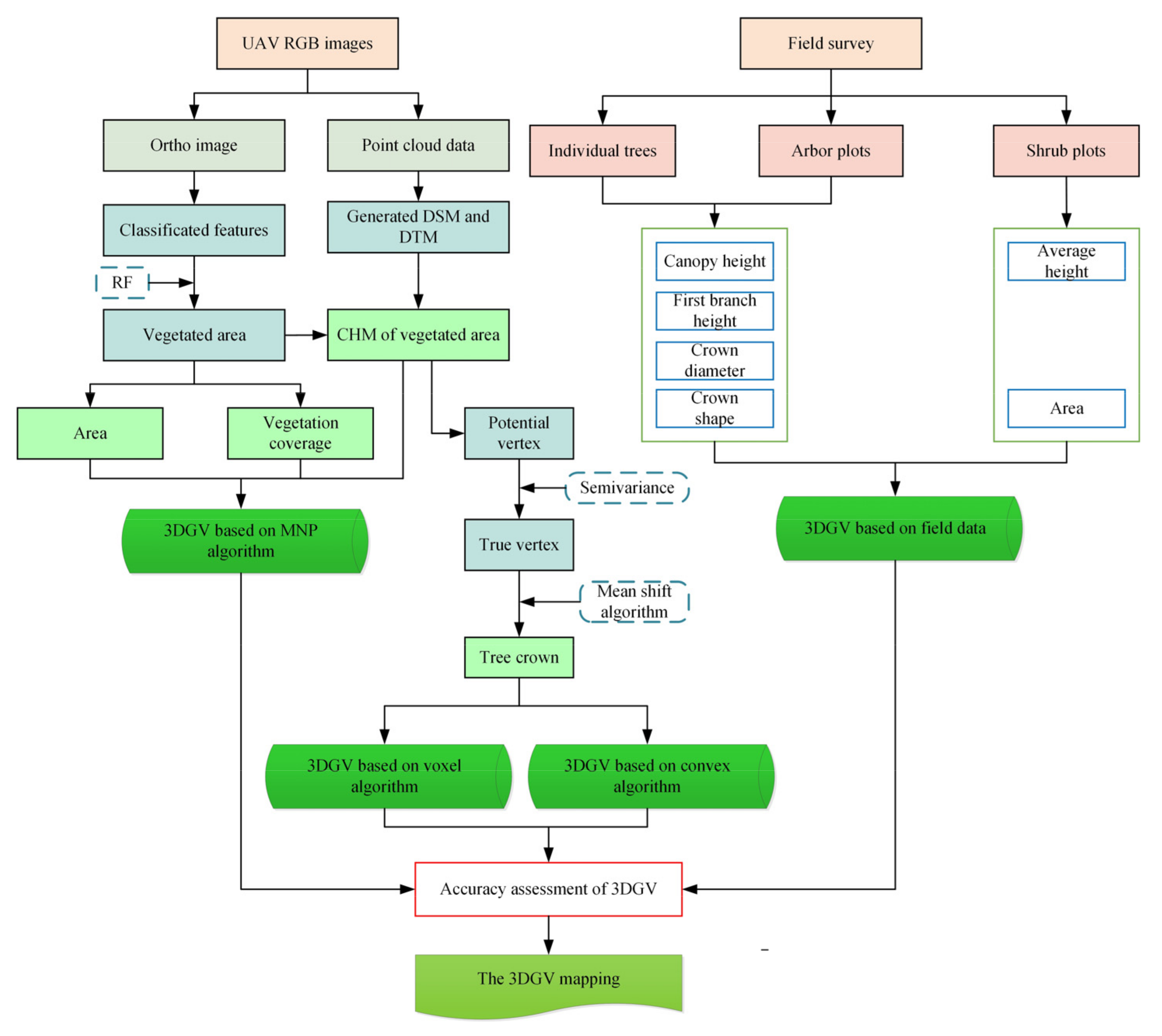
Figure 1. Workflow for 3DGV estimation based on UAV RGB images.
Forests 14 00752 g001
Figure 2. Location of YueYaTan Park.
Forests 14 00752 g002
Figure 3. The plots in YueYaTan Park.
Forests 14 00752 g003
Figure 4. Vegetation distribution in YueYaTan Park.
Forests 14 00752 g004
Figure 5. DSM and DTM of the vegetated area: (a) DSM of the vegetated area; (b) DTM of the vegetated area.
Forests 14 00752 g005
Figure 6. The diagram of the Convex hull algorithm.
Forests 14 00752 g006
Figure 7. The CHM of the vegetated area.
Forests 14 00752 g007
Figure 8. Accuracy assessment of the canopy height: (a) Scatter diagram of the H_CHM and H_FD in plots; (b) bias, relative bias, RMSE, and relative RMSE of the MH_FD, MCH_FD, and H_CHM in plots; (c) scatter diagram of the H_CHM and H_FD; (d) bias, relative bias, RMSE, and relative RMSE of the MH_FD, MCH_FD, and H_CHM in individual trees.
Forests 14 00752 g008
Figure 9. Vegetation coverage of the vegetated area.
Forests 14 00752 g009
Figure 10. Accuracy assessment of 3DGV: (a) Scatter diagram of 3DGV_MNP, 3DGV_Con, and 3DGV_Voxel in plots; (b) bias, relative bias, RMSE, and relative RMSE of 3DGV_MNP, 3DGV_Con, and 3DGV_Voxel in plots; (c) scatter diagram of 3DGV_MNP, 3DGV_Con, and 3DGV_Voxel in individual trees; (d) bias, relative bias, RMSE, and relative RMSE of 3DGV_MNP, 3DGV_Con, and 3DGV_Voxel in individual trees.
Forests 14 00752 g010
Figure 11. The 3DGV maps: (a) The results of the MNP algorithm; (b) the results of the Convex hull algorithm; (c) the results of the Voxel algorithm.
Forests 14 00752 g011
Figure 12. The detected vertex and the segmentation results of the sample plots: (ah) The detected vertex of plot 1 to plot 8; (i) the detected vertex of individual trees.
Forests 14 00752 g012
Figure 13. The areas with high vegetation density.
Forests 14 00752 g013
Table 1. Abbreviations of factors in this paper.
AbbreviationMeaning
H_FDThe tree height of measured field data.
H_CHMThe canopy height of CHM in our works.
MH_FDThe mean tree height derived from field data.
MCH_FDThe mean canopy height derived from field data.
3DGV_FDThe 3DGV calculated by geometrical formulas.
3DGV_ConThe 3DGV estimated based Convex hull algorithm.
3DGV_VoxelThe 3DGV estimated based Voxel algorithm.
3DGV_MNPThe 3DGV estimated based on the Mean neighboring of pixels algorithm.
Table 2. The details of sample plots.
PlotsTotal NumberPlots Size/m2Vegetation Size/m
Arbor plots7256Tree height > 3
Shrub plots3256Tree height < 3
Individual trees31
Table 3. The 3DGV Calculation Equations of Different Tree Species.
Tree SpeciesGeometrical
Morphology
Calculation EquationDescription
Metasequoia glyptostroboides Hu and W.cone Π a 2 b / 12 a represents crown diameter and b represents crown height.
Salix babylonica L.
Elaeis guineensis Jacq.
ovoid Π a 2 b / 6
Osmanthus fragrans Makino.
Cinnamomum japonicum Sieb.
Ficus microcarpa L.f.
sphere Π a 2 b / 6
Elaeocarpus decipiens Linn.
Cycas revoluta Thunb.
flabellate Π 2 a 3 a 2 × 4 a 2 b 2 / 3
Table 4. Vegetation indices.
Vegetation IndicesDescription
E X G = 2 × ρ g r e e n ρ r e d ρ b l u e ρ g r e e n ,   ρ r e d , ρ b l u e represent the three bands of red, green, blue, respectively reflectance.
N G R D I = ρ g r e e n ρ r e d ρ r e d + ρ g r e e n
N G B D I = ρ g r e e n ρ b l u e ρ b l u e + ρ g r e e n
R G R I = ρ r e d ρ g r e e n
V D V I = 2 × ρ g r e e n ρ r e d ρ b l u e 2 × ρ g r e e n + ρ r e d + ρ b l u e
Table 5. Calculation Equations of texture features.
Texture FeaturesDescription
M E A = i = 0 N 1 j = 0 N 1 i × P i , j N is the gray level; i and j are the gray value of two neighboring resolution cells separated by the distance occurring in the image, respectively; i , j stands for the times the number of the gray value i and j were neighbors; P i , j is the normalized gray value spatial dependence matrix.
S T D =   i = 0 N 1 j = 0 N 1 i m e a n 2 × P i , j
H O M = i = 0 N 1 j = 0 N 1 P i , j 1 + i j 2  
D I S = i = 0 N 1 j = 0 N 1 P i , j × i j  
E N T = i = 0 N 1 j = 0 N 1 P i , j × ln P i , j
A S M = i = 0 N 1 j = 0 N 1 P i , j 2
Table 6. Classification Confusion Matrix and Classification Accuracy.
ClassesVegetationNon-VegetationUA/%
Vegetation10101498.63
Non-Vegetation18130998.64
PA/%98.2498.94
OA/%98.64
Kappa0.98
Disclaimer/Publisher’s Note: The statements, opinions and data contained in all publications are solely those of the individual author(s) and contributor(s) and not of MDPI and/or the editor(s). MDPI and/or the editor(s) disclaim responsibility for any injury to people or property resulting from any ideas, methods, instructions or products referred to in the content.