Comprehensive Decision Index of Logging (CDIL) and Visual Simulation Based on Horizontal and Vertical Structure Parameters

Abstract

The comprehensive indexes approach based on stand structure parameters is mainly used to select trees for harvest. However, these indexes do not consider the comprehensive impact of horizontal and vertical structures, leading to an incomplete analysis of the forest structure and an inaccurate selection of trees for harvest. To solve this problem, we constructed a comprehensive decision index of logging (CDIL), integrating horizontal and vertical structure parameters which can identify harvest trees more scientifically. In this study, we took the Shanxia Forest Farm in the Jiangxi Province of China as the experimental area and used mixed broadleaf/conifer forests at different ages as our experimental sample. We selected eight horizontal and vertical spatial structure parameters to establish an efficient, objective, and accurate comprehensive decision index of logging. We combined 3D visualization technology to realize the dynamic visualization simulation of the index at different intensities of tending and felling management. The results indicated that the proposed CDIL-index could effectively optimize the forest spatial structure. From the perspective of stand structure adjustment, the optimal thinning intensity was 20%. The average CDIL in each plot decreased by more than 80% after logging, while the change range of each plot was between 30% and 70% after the F index was applied to implement tending and logging. The CDIL was 11.4% more accurate in selecting trees for harvesting than the F index. In this study, the main conclusion is that the CDIL would enable forest managers to more accurately choose trees for harvesting, leading to forest adjustment that would reduce the competition pressure among trees and improve the distribution and health of trees, possibly making the forest structure more stable.

1. Introduction

As the most basic and important feature of forest ecosystems, the forest structure has spatial and nonspatial characteristics [1]. An important part of forest management is forest structure analysis since it facilitates our understanding of forest communities [2]. The forest spatial structure is more important than the nonspatial structure since the spatial structure largely determines the distribution and competition of trees, and reflects the health of the trees, the diversity of tree species, and the stability of the stand [3]. In recent years, to transform large areas of coniferous pure forests with low ecological and economic benefits into broad-leaved mixed forests with high biodiversity and stability, European forestry-developed countries, such as Germany and the United Kingdom, have carried out research on forest spatial structure adjustment with selective harvest trees as the main measure [4,5,6,7,8]. North American countries have paid attention to analyzing the forest spatial structure, and providing the basis for forest growth and stand dynamic simulation [6,9,10]. These studies have shown that the analysis and optimization of the forest spatial structure is the most active research field [7].

An important issue in forest management is forest thinning, which can directly affect the stand structure. By regularly cutting some trees in the forest, we can improve the competitive environment of the trees, enhance the living space of the trees and the forest structure, and adjust the total amount and distribution mode of forest resources [11,12,13]. Trees of different species, in different health conditions, and of different diameter classes can respond differently to the distribution of natural resources and the improved competitive environment [14,15]. Forest thinning may change the understory light, temperature, and humidity conditions, thereby improving the physical and chemical properties of the soil, promoting the regeneration of undergrowth vegetation, maintaining soil fertility, and providing higher ecological and environmental benefits as well as social and economic benefits [16]. However, unreasonable thinning may have negative consequences, such as damaging vegetation regeneration, interfering with nutrient cycles, hindering animal adaptation, increasing forest pests, and even causing forest fires [17,18,19]. Therefore, how to effectively optimize the stand spatial structure, scientifically select harvest trees, and practice reasonable tending and felling is the premise for maintaining stand stability for the sake of sustainable development [20,21].

At the core of thinning is the selection of trees to be harvested [22]. In recent decades, a large number of scholars have proposed some forest management methods, including the comprehensive indexes approach [23], the stem number guide curve [24], and target tree-oriented management [25]. Although each of these methods include several parameters, they lack information about the spatial structure. To evaluate characteristics of the stand spatial structure, recently, Ye et al. [21], and Pastorella et al. [26] developed comprehensive indexes to evaluate the characteristics of the stand spatial structure based on several common parameters, such as the U-index, the M-index, and the D-index. However, none of these comprehensive indexes considers the impact of the stand vertical structure. For example, Li et al. used the composite index to select harvest trees according to the bivariate distributions of the three spatial parameters (i.e., the U, the M, and the D index) [22]. Though the three spatial structure indicators are used extensively, they are not comprehensive enough. Courbaud et al. simulated the influence of different selective cutting methods, including cluster selective cutting and single tree selective cutting, on the spatial structure and growth of Norwegian spruce uneven-aged forests in the French Alps Mountains [27]. Cao et al. used multiplication and division to carry out multiobjective planning for the selected spatial structure parameters and proposed the objective function for optimizing the stand spatial structure and exploring the stand spatial structure of trees of different ages and different thinning intensities [28]. Lv et al. used multiplication and division to develop a comprehensive cutting index to verify the effectiveness of adjusting the spatial structure of the stand. The index put forward by Lv et al. covered eight parameters, including horizontal spatial structure parameters, which produced good results. Therefore, this paper used the index constructed by Lv et al. for comparison [29]. In most of these studies, stand spatial and nonspatial structure indicators or horizontal structure parameters were selected to construct the cutting index [20,22,28,29]. They did not consider the comprehensive effects of vertical spatial structural parameters and other structural parameters. However, the vertical spatial structure parameters of the stand play an important role in improving the forest growth space and accurately and efficiently selecting trees for harvest.

In a study on the setting of sample plots for forest structure optimization, Dong selected four permanent plots, each measuring 100 m × 100 m [20]. Ahmad et al. selected 82 sample plots, some measuring 30 m × 30 m and some of 20 m × 20 m [30]. Bhandari et al. selected 30 sample plots measuring 40 m × 40 m each [31]. These studies had different sample plot sizes due to different topographic factors. In our study, on the basis of the influence of topographic and human factors in the study area, we selected five sample plots of 50 m × 50 m each.

The purpose of our study was to put forward a new comprehensive decision index of logging (CDIL) based on horizontal and vertical spatial parameters of the stand. We then employed the comprehensive index to determine the harvest trees for the five plots of the Shanxia Forest Farm in Jiangxi Province of China, determined the number of harvest trees in the plot according to the optimal thinning intensity, and then conducted a thinning simulation, The development of the CDIL involved four steps: (1) comprehensively analyzing and judging harvest trees in the stand, (2) identifying any correlation between vertical spatial structure parameters and the CDIL, and quantifying the advantages of the CDIL in adjusting the stand spatial structure, (3) comparing the CDIL with the logging index by Lv et al., and calculating the accuracy of the CDIL in selecting harvest trees [21], and (4) carrying out the dynamic visual simulation of stand management, and evaluating the simulation results, based on Unreal Engine 4 [32].

The CDIL helps to adjust the spatial structure of the stand and transform the unreasonable spatial structure of the forest into an optimal state. Moreover, visual simulation enables managers to respond in a timely manner to the changes and distribution of the spatial structure characteristics of the forest stand and the problems that may occur in the management process so as to modify the forest management plan when necessary.

2. Materials and Methods

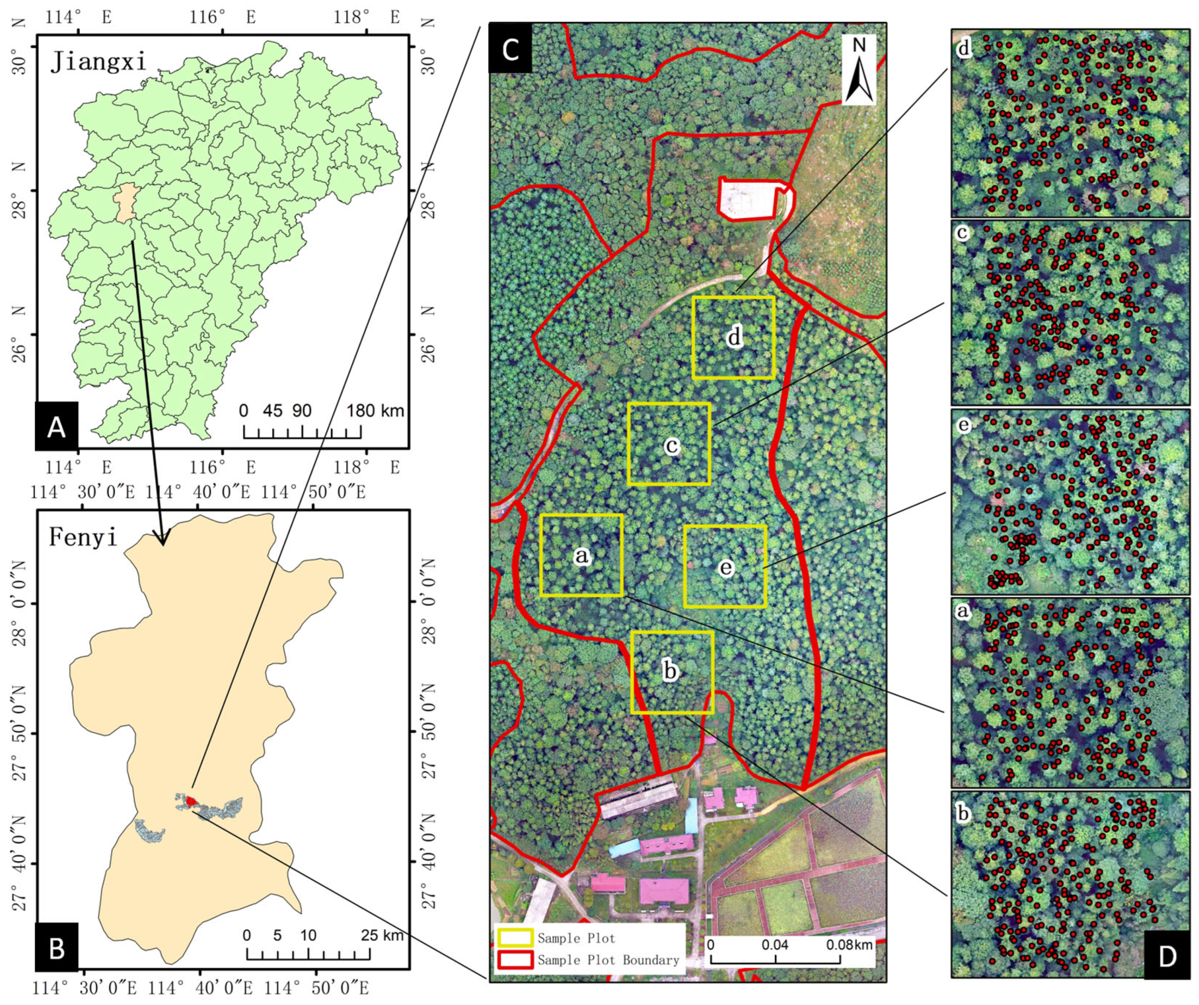
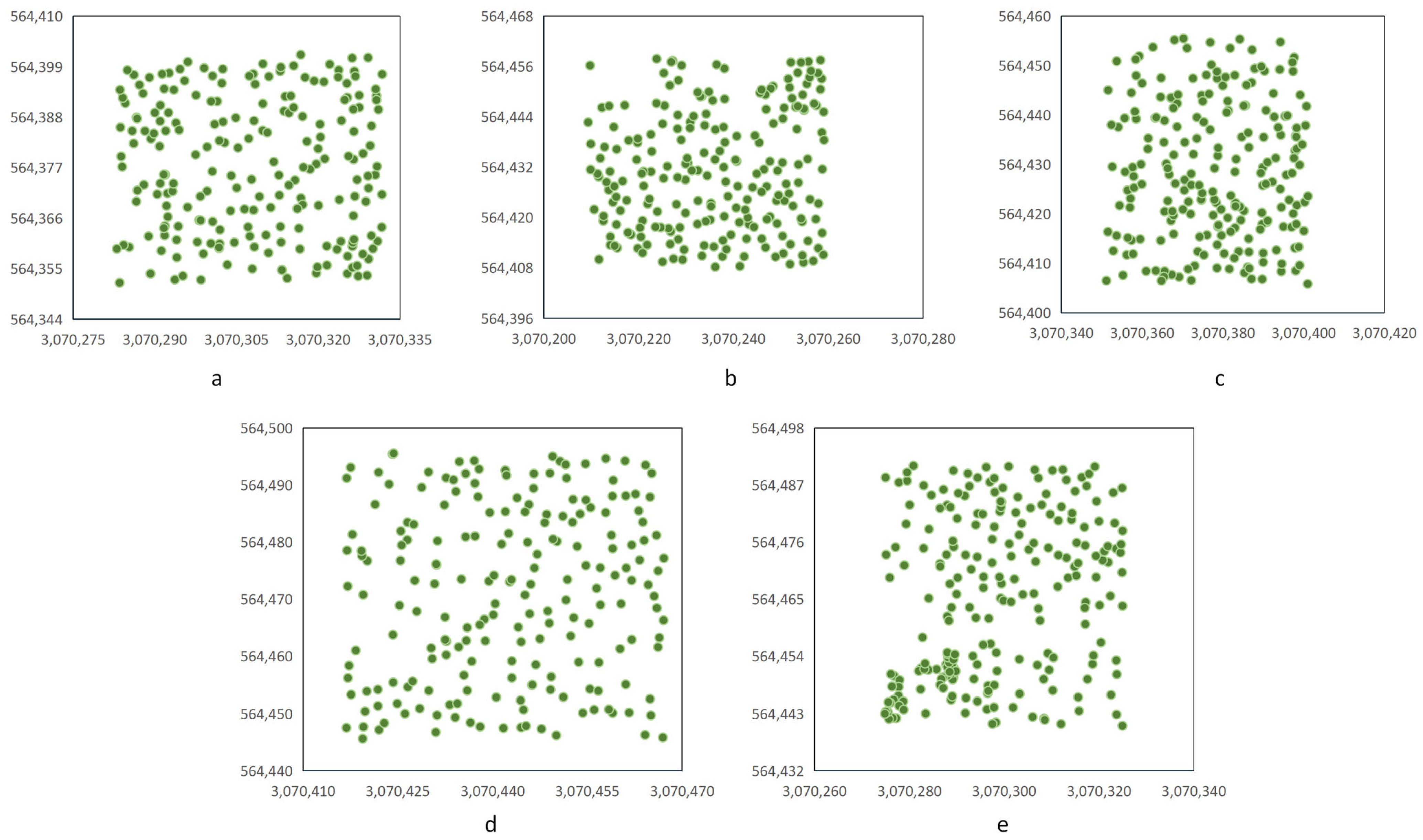
2.1. Study Areas

The study area was located in Shanxia Experimental Forest Farm in the southwest of Fenyi County, Xinyu City, Jiangxi Province, China (Figure 1). The region has 1920 kinds of plants, and the forest coverage rate is 64.3%. The zonal vegetation is the midsubtropical evergreen broad-leaved forest. The dominant tree species are Cunninghamia lanceolate, Pinus massoniana, and Schima Superba. The area belongs to the subtropical monsoon climate with sunshine. The frost-free period is of 270 days. It has abundant rainfall, with an annual precipitation of 1600 mm and a mean annual temperature of 15~17 °C. The soil in the forest farm is fertile, and the soil type is mainly loam soil (Figure 1).

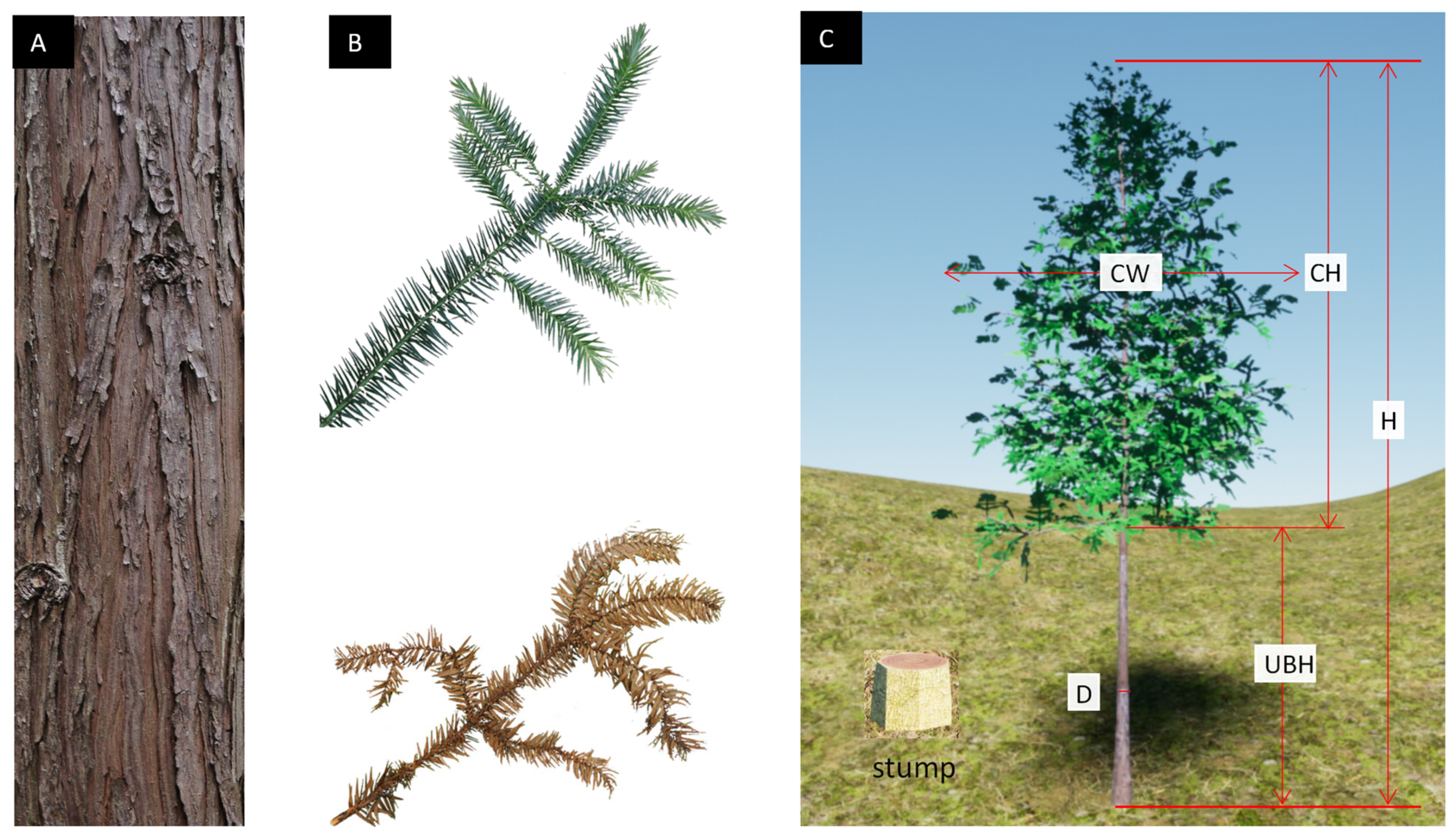
2.2. Data Collection

In May 2022, five fixed plots, each measuring 50 m × 50 m, with artificial uneven-aged coniferous and broad-leaved mixed forests were set up on the forest farm. In each plot, the relative coordinates (x, y, z) of the root of each tree were measured using the total station and prism. The tree species were recorded and provided by forest farm staff. The diameter at breast height (DBH) of each tree, was measured using the DBH tape measure. A laser altimeter was used to measure the tree height(H) and the height under the living branches (UBH) of trees. The crown widths (CWs) of the trees were measured using a box staff.

Table 1. The basic stand characteristics of the five plots.

Plots	Plot Area (hm2)	Stand Density (Trees/ha)	Average DBH (cm)	Average Height (m)	Average Crown Width (m)	Average UBH (m)	Number of Tree Species
a	0.25	215	17.9	12.4	3.7	4.8	8
b	0.25	216	16.9	11.4	3.2	4.1	16
c	0.25	221	17.7	14.6	3.4	4.5	6
d	0.25	203	18.1	12.4	3.8	4.3	9
e	0.25	225	16.9	12.9	3.6	4.5	7

lists the basic stand characteristics of the five plots. To avoid inaccurate calculation results of the single tree competition index, we set up 5 m buffer zones among the five plots. To build 3D models of the trees, we used a digital camera to photograph the bark and leaf texture of trees, shrubs, and herbs.

2.3. Data Analysis

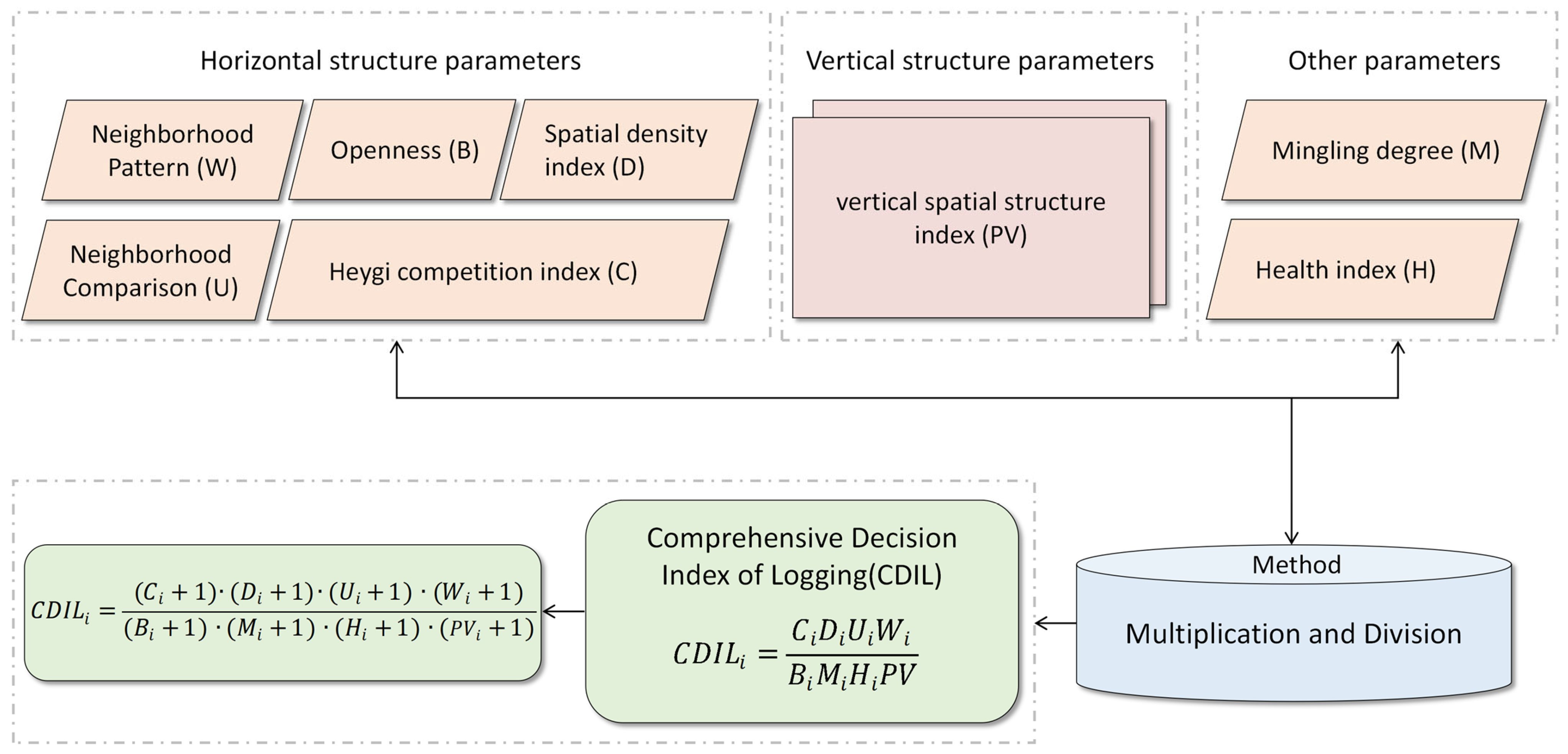
2.3.1. Construction of the Comprehensive Decision Index of Logging (CDIL)

The CDIL consists of eight parameters: neighborhood Pattern (W), neighborhood comparison (U), mingling degree (M), openness (B), health index (H), spatial density index (D), Heygi competition index (C), and vertical spatial structure parameter (PV). They, respectively, reflect the following eight horizontal and vertical structural parameters: the spatial distribution pattern of trees, the diversity of tree species, the degree of crowding, the competitiveness of trees, the spatial advantage degree, openness, the health of trees, and the number of trees covered by adjacent trees.

Table 2. Descriptions of the eight horizontal and vertical structure parameters.

Type	Indexes	Abbreviation	Equation	Describe/Rule	References
Horizontal structure parameters	Neighborhood pattern	W	${\mathrm{W}}_{\mathrm{i}}=\frac{1}{\mathrm{n}}{\displaystyle \sum _{\mathrm{j}=1}^{\mathrm{n}}}{\mathrm{Z}}_{\mathrm{i}\mathrm{j}}$	It is used to describe the evenness of adjacent trees around the target tree. ${\mathrm{Z}}_{\mathrm{i}\mathrm{j}}=\left\{\begin{array}{c}1, \mathrm{When} \mathrm{the} \mathrm{angle} \mathrm{j} \mathrm{was} \mathrm{smaller} \mathrm{than} \mathrm{the} \mathrm{standard} \mathrm{angle} {\mathrm{\alpha }}_0\\ 0, \mathrm{otherwise}\end{array}\right.$	[26,33,34]
	Neighborhood comparison	U	${\mathrm{U}}_{\mathrm{i}}=\frac{1}{\mathrm{n}}{\displaystyle \sum _{\mathrm{j}=1}^{\mathrm{n}}}{\mathrm{k}}_{\mathrm{i}\mathrm{j}}$	It reflects the dominance of trees in the growth process. ${\mathrm{k}}_{\mathrm{i}\mathrm{j}}=\left\{\begin{array}{c}1, \mathrm{If} \mathrm{the} \mathrm{adjacent} \mathrm{tree} \mathrm{i} \mathrm{was} \mathrm{larger} \mathrm{than} \mathrm{the} \mathrm{reference} \mathrm{tree}\\ 0, \mathrm{otherwise}\end{array}\right.$	[35]
	Openness	B	${\mathrm{B}}_{\mathrm{i}}=\frac{1}{\mathrm{n}}{\displaystyle \sum _{\mathrm{j}=1}^{\mathrm{n}}}\frac{{\mathrm{D}}_{\mathrm{i}\mathrm{j}}}{{\mathrm{H}}_{\mathrm{j}}}$	It is used to describe the growth of trees in the plot space.	[36]
	Spatial density index	D	${\mathrm{D}}_{\mathrm{i}}=1-\frac{{\mathrm{r}}_{\mathrm{i}}}{{\mathrm{r}}_{\mathrm{m}\mathrm{a}\mathrm{x}}}$	It refers to the degree of tree crowding in the spatial structure unit.	[37]
	The Heygi competition index	C	${\mathrm{C}}_{\mathrm{i}}={\displaystyle \sum _{\mathrm{j}=1}^{\mathrm{n}}}\frac{{\mathrm{D}}_{\mathrm{j}}}{{\mathrm{D}}_{\mathrm{i}}·{\mathrm{L}}_{\mathrm{i}\mathrm{j}}}$	It is defined as the distance between the target tree and the the competitive tree and the ratio of the diameter of the competitive tree to the target tree.	[32]
Vertical structure parameters	Vertical spatial structure parameter	PV	${\mathrm{P}\mathrm{V}}_{\mathrm{i}}={\displaystyle \sum _{\mathrm{j}=1}^{\mathrm{n}}}\left\{\begin{array}{c}{\tan }^{-1}\left(\frac{\left({\mathrm{H}}_{\mathrm{j}}-{\mathrm{H}}_{\mathrm{i}}\right)}{{\mathrm{d}\mathrm{i}\mathrm{s}\mathrm{t}}_{\mathrm{i}\mathrm{j}}}\right)\\ -\mathrm{arctg}\left(\frac{\left({\mathrm{H}}_{\mathrm{j}}-{\mathrm{H}}_{\mathrm{i}}\right)}{{\mathrm{d}\mathrm{i}\mathrm{s}\mathrm{t}}_{\mathrm{i}\mathrm{j}}}\right)\end{array}\right.$	It indicates the degree to which the target tree is covered by the competitive tree.	[38]
Other parameters	Mixing degree	M	${\mathrm{M}}_{\mathrm{i}}=\frac{1}{\mathrm{n}}{\displaystyle \sum _{\mathrm{j}=1}^{\mathrm{n}}}{\mathrm{v}}_{\mathrm{i}\mathrm{j}}$	It describes the isolation degree of tree species in the mixed forest. ${\mathrm{v}}_{\mathrm{i}\mathrm{j}}=\left\{\begin{array}{c}1, \mathrm{The} \mathrm{target} \mathrm{tree} \mathrm{i} \mathrm{and} \mathrm{the} \mathrm{adjacent} \mathrm{tree} \mathrm{j} \mathrm{are} \mathrm{different} \mathrm{species}\\ 0, \mathrm{otherwise}\end{array}\right.$	[26,36]
	Health index	H	${\mathrm{H}}_{\mathrm{i}}=\frac{1}{\mathrm{n}}{\displaystyle \sum _{\mathrm{j}=1}^{\mathrm{n}}}{\mathrm{x}}_{\mathrm{i}\mathrm{j}}$	It indicates that when the health of the target tree i is better than the that of adjacent tree j, ${\mathrm{x}}_{\mathrm{i}\mathrm{j}}$ = 1, otherwise ${\mathrm{x}}_{\mathrm{i}\mathrm{j}}$ = 0.	[39]

describes the eight horizontal and vertical structure parameters. Figure 2 presents the development process of the CDIL.

All the quantitative horizontal and vertical indexes described above are significant for stand spatial structure adjustment. To select the harvest trees, the relationship between each target tree and its four nearest trees should be evaluated. Therefore, coupled with the above eight stand structure parameters, we used multiplication and division to construct a comprehensive decision index of logging to comprehensively analyze the trees. The formula is:

$${CDIL}_i=\frac{C_i{D}_i{U}_i{W}_i}{B_i{M}_i{H}_{i}PV},$$

(1)

When Formula (1) is applied, the value of factors such as $M_i$ and $W_i$ may be zero, resulting in large errors in the results. Therefore, according to the method of multiplication and division, 1 is added to all parameters in Formula (1) to get Formula (2):

$${CDIL}_i=\frac{{(C}_i+1){·(D}_i+1){·(U}_i+1)·(W_i+1)}{{(B}_i+1)·(M_i+1)·(H_i+1)·({PV}_i+1)},$$

(2)

The formula for the average comprehensive decision index of logging the stand is stated as:

$$CDIL=\frac{1}{N}{\displaystyle {\sum }_{i=1}^N}{CDIL}_i,$$

(3)

where ${CDIL}_i$ represents the comprehensive decision index of logging; $CDIL$ represents the average comprehensive decision index of logging of the stand; and $C_i$, $D_i$, $U_i$, $W_i$, $B_i$, $M_i$, $H_i$, and ${PV}_i$ represent, respectively, the Heygi competition index, the spatial density index, neighborhood comparison, neighborhood pattern, openness, the mingling degree, the health index, and the vertical spatial structure parameter of the target tree.

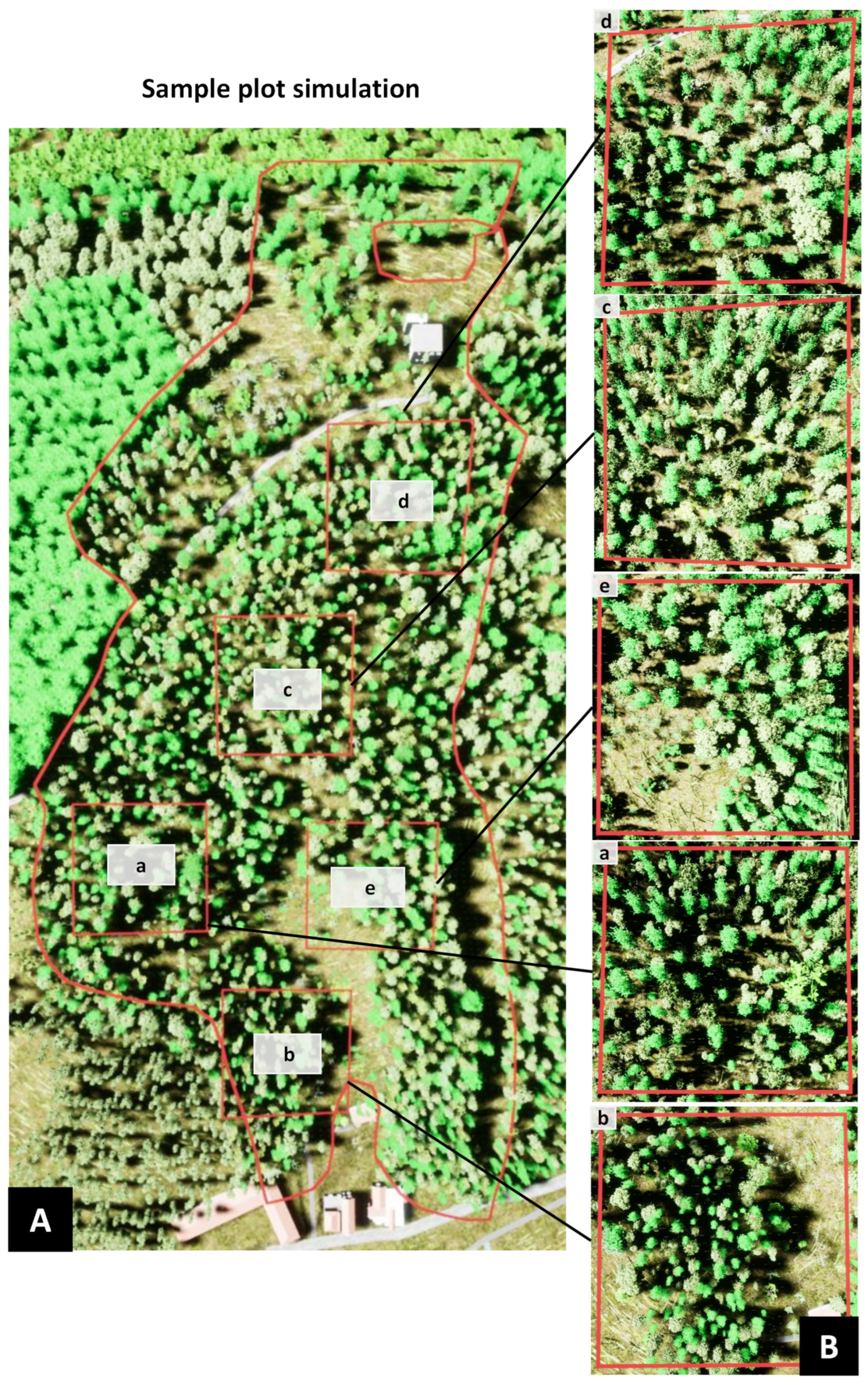
2.3.2. Dynamic Visual Simulation of Management

Using Unreal Engine 4 (https://www.unrealengine.com/zh-CN, accessed on 10 December 2023), which is an efficient and versatile game development engine launched by Epic Games, we can directly preview the development effect. We connect to the MySQL database with UE4 and read the stand data table. The three-dimensional model of a tree is divided into two parts, the trunk and the crown. The original point of the coordinates of the trunk and the crown of the tree classification model is assumed to be at the bottom. The initial DBH of the trees in the forest is D₀, the height of the trees is H₀, the crown width is CW₀, the height under branches is UBH₀, and the crown height is CH₀. The trunk diameter at breast height scaling factor DBH_XY_scale = D₀/D (D is the diameter at breast height of the initial model), the height under the branch scaling coefficient UBH_Z_scale = UBH₀/UBH (UBH is the height under the branch of the initial model), the scaling coefficient of the crown width CW_ XY_scale = CW₀/CW (CW is the crown size of the initial model), and the crown height scaling coefficient CH_Z_scale = CH₀/CH (CH is the crown height of the initial model). Figure 3 presents the virtual reality scene of the real initial forest scene of the five sample plots.

On the basis of the index calculation formula listed in Table 2 and the UE4 blueprint function script, which is a visual script that provides an intuitive, node-based interface and realizes code programming by dragging and dropping nodes, a function for calculating the eight stand structural parameters and the CDIL is written. As per the calculation results, we determined the trees for harvest in each plot according to thinning intensities of 10%, 20%, and 30% of the number of trees and established the cutting data table. We then removed the harvest trees determined by each thinning intensity value and replaced them with stump models. The stand structure changed after cutting. We recalculated the stand structure parameters and the CDIL and analyzed the accuracy of harvest tree selection and the results of stand structure adjustment.

According to the blueprint function script, the timeline animation event, and the forest growth model library (the forest growth model library used the growth model that conforms to the growth of the dominant species provided by the forest farm locally), the tree growth functions were written and the growth of stands of different ages was dynamically simulated, in which the DBH growth model and the UBH growth model were used for the tree trunk, while the CW growth model and the CH growth model were used for the tree crown. We assume that the DBH of trees of different ages is D_i, the tree height is H_i, the crown width is CW_i, the height under branches is UBH_i, and the crown height is CH_i. The DBH scaling coefficient of the trunk is xiongjing_XYscale = D_i/D_i-1 (i > 1), and the UBH scaling coefficient zhixiagao_Zscale = UBH_i/UBH_i-1 (i > 1). The crown width scaling coefficient guanfu_XYscale = CW_i/CW_i-1 (i > 1), and the crown height scaling coefficient guangao_Zscale = CH_i/CH_i-1(i > 1).

3. Results

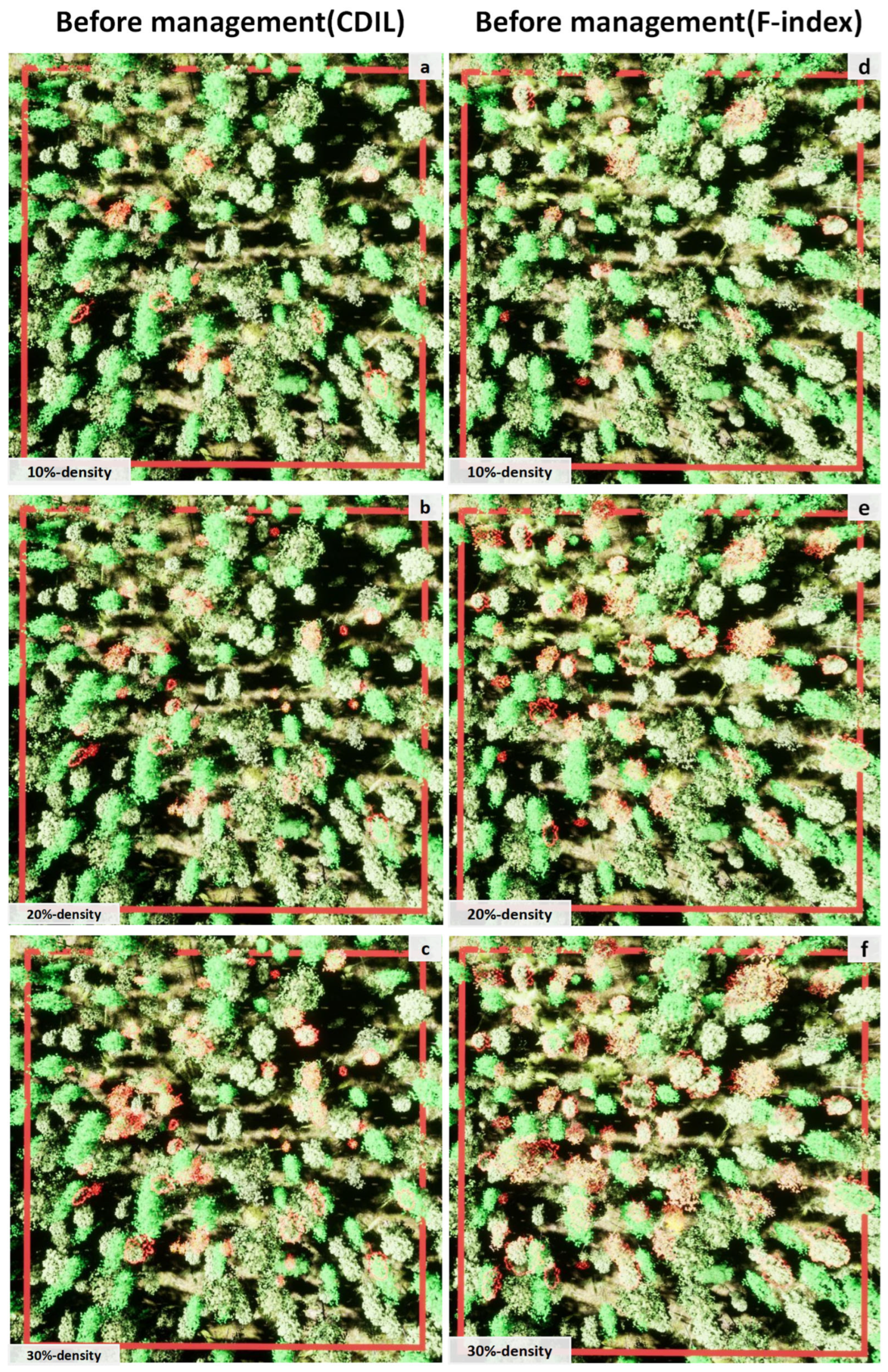
3.1. Determination of Logging

To identify the accuracy of the CDIL in selecting trees for harvest, we selected the logging index with comprehensive indicators by Lv et al. [29] for comparison.

The thinning intensities of 10%, 20%, and 30% were simulated according to the growth and quality of the stand in the plot. The harvest trees were selected according to the calculation results of the CDIL and the F index [29]. The average index when 10% of the trees were identified for harvest in the five plots is illustrated in

Table 3. The average index when 10% of the trees were identified for harvest in the five plots.

Plots	Harvest Tree Number		W-Index		U-Index		M-Index		B-Index		H-Index		D-Index		C-Index		PV-Index
	CDIL	F Index	CDIL	F Index	CDIL	F Index	CDIL	F Index	CDIL	F Index	CDIL	F Index	CDIL	F Index	CDIL	F Index	CDIL
a	48, 197, 103, 47, 49, 198, 70, 102, 56, 25, 41, 114, 7, 16, 2, 55, 121, 108, 36, 180, 69	25, 149, 1, 213, 55, 206, 106, 118, 132, 35, 161, 119, 40, 8, 169, 215, 9, 66, 81, 188, 184	0.59	0.58	0.66	0.65	0.52	0.61	0.2	0.23	0.29	0.39	0.94	0.81	6.40	9.48	1.33
b	210, 188, 204, 9, 181, 167, 165, 205, 182, 192, 137, 50, 209, 121, 202, 89, 88, 189, 142, 166, 197	82, 180, 157, 108, 117, 20, 153, 53, 211, 11, 58, 126, 3, 40, 176, 8, 54, 56, 13, 107, 139	0.61	0.49	0.69	0.81	0.28	0.59	0.31	0.25	0.32	0.51	0.83	0.7	3.92	3.47	1.16
c	149, 177, 108, 13, 107, 178, 127, 82, 183, 33, 193, 55, 35, 58, 42, 122, 20, 78, 95, 18, 126, 83	177, 107, 43, 215, 57, 126, 106, 148, 129, 185, 191, 45, 71, 145, 189, 11, 214, 82, 9, 186, 209, 199	0.56	0.55	0.75	0.68	0.45	0.59	0.2	0.23	0.24	0.47	0.86	0.82	8.88	3.84	2.06
d	51, 118, 97, 99, 179, 164, 184, 107, 7, 91, 50, 82, 158, 182, 53, 189, 49, 18, 77, 136	7, 80, 175, 164, 57, 67, 38, 101, 117, 126, 12, 193, 100, 55, 181, 28, 4, 33, 169, 180, 42	0.56	0.43	0.81	0.79	0.39	0.62	0.22	0.26	0.14	0.35	0.78	0.73	8.14	3.38	2.76
e	195, 190, 161, 167, 171, 165, 216, 181, 222, 40, 208, 197, 193, 203, 225, 2, 196, 215, 185, 186, 192, 223	12, 43, 134, 32, 88, 18, 110, 197, 221, 145, 102, 106, 223, 154, 108, 98, 91, 195, 24, 60, 136, 169, 51	0.59	0.58	0.63	0.43	0.15	0.53	0.24	0.25	0.29	0.56	0.85	0.74	4.17	2.48	1.02

. First, trees numbered 13, 17, 19, 23, and 37, marked as unhealthy, broken, and withered in the plot survey, had to be cut down. According to the value of the CDIL, it was concluded that the comprehensive decision index of the tree numbered 177 was the largest. Its H-index was 0.25, close to zero, and thus it could be regarded as an unhealthy tree. The spatial density index was 0.99, which meant the area around it was extremely crowded and not conducive to its growth. Competitive tree numbered 94 was simultaneously squeezed by trees numbered 178 and 93. Therefore, it was removed. The CDIL was recalculated after removing the trees, and this operation was repeated until the forest spatial structure after the trees were cut reached the ideal state of management objectives.

For a target tree to be in an advantageous position, its competition neighborhood comparison should not have been greater than 0.25 [22,24]. In the five plots, the average W-index values of the harvest trees were all above 0.5 and the C-index was large. Therefore, identifying them as harvest trees reflected the rule of cutting small trees while retaining large ones. The average H-index was close to zero, indicating that most of the selected trees were unhealthy and this reflected the necessity of cutting the inferior trees and retaining the superior ones. In terms of the average D-index, the values of the five plots were all higher than 0.7. The D-index of Plot a was close to one. Plot a was in an extremely crowded state, indicating the need to reduce the density and retain sparsity. The PV-index was small, implying that the trees identified for harvest were considerably covered by the surrounding trees and should be harvested.

The harvest trees selected by the CDIL were different from those selected using the F index. A W-index close to 0.5 indicates that the distribution pattern of the stand was random and the stand tended to be stable [40]. The harvest trees selected by the CDIL in Plots a-e had average W-indexes of 0.59, 0.61, 0.56, 0.56, and 0.59, respectively, which belonged to aggregated distribution. However, the harvest trees selected by the F index had average W-indexes of 0.58, 0.49, 0.55, 0.43, and 0.58, respectively. Compared with the CDIL, the F index produced a result closer to 0.5, signifying that Plot b had random distribution and no adjustment was required. This indicates that the trees identified for harvest by the CDIL did not conform to the random distribution and the adjustment range was larger than the F index. The larger the U-index, the less is the growth advantage [41]. The average U-indexes of the harvest trees selected by the CDIL in the five plots were larger than the harvest trees selected by the F index, with the exception being Plot b. This indicated that the harvest trees selected by the CDIL were more unfavorable to growth than those selected by the F index. The harvest trees selected by the CDIL in the five plots had average M-indexes of 0.09, 0.31, 0.14, 0.23, and 0.38, which were smaller than those of the harvest trees selected by the F index. To improve the diversity of tree species, trees with a small M-index should be harvested. However, the harvest trees selected by the F index in the five plots had M-indexes greater than 0.5, which was inconsistent with the research of other scholars [3,36,42]. The average H-index of the harvest trees selected by the CDIL in each of the five plots was close to zero, indicating that the trees identified for harvest were unhealthy. However, the harvest trees selected by the F index had an H-index close to 0.5, so it was difficult to judge the health status of the trees. The harvest trees selected by the CDIL in Plots a, c, d, and e had an average B-index smaller than that of the harvest trees selected by the F index. The trees selected for harvest by the CDIL in Plots a-e had average D-indexes of 0.13, 0.13, 0.04, 0.05, and 0.11, respectively, and all values were greater than the D-indexes of the harvest trees selected by the F index. The B-index and the D-index indicated that the harvest trees selected by the CDIL were distributed in the more clustered areas. The average C-index of the harvest trees selected by the CDIL in each of Plots b, c, d, and e was larger than that of the harvest trees selected by the F index, indicating that the harvest trees selected by the CDIL have a higher competition pressure, which was not conducive to the growth of trees.

These results indicate that the CDIL constructed by comprehensively considering the horizontal spatial structure parameters and the vertical spatial structure parameters can help in a more reasonable and accurate selection of harvest trees.

3.2. Results of Vertical Spatial Structure Parameters

We analyzed the calculation results of the eight spatial structure parameters and the CDIL of stands in the five plots. The relative strength of the CDIL affected by the stand spatial structure index was calculated by using the grey correlation analysis method in the multifactor statistical analysis [32].

Table 4. The coefficient of correlation between stand spatial structure parameters and the CDIL.

Plots	M-Index	U-Index	W-Index	H-Index	D-Index	C-Index	B-Index	PV-Index
a	0.356	0.353	0.351	0.352	0.353	0.842	0.345	0.369
b	0.555	0.531	0.544	0.549	0.544	0.747	0.528	0.576
c	0.672	0.726	0.688	0.735	0.706	0.914	0.761	0.696
d	0.954	0.828	0.795	0.834	0.789	0.609	0.983	0.862
e	0.653	0.575	0.563	0.547	0.551	0.734	0.605	0.601
average	0.638	0.602	0.588	0.603	0.589	0.769	0.644	0.621

presents the coefficient of correlation between the spatial structure parameters of stands and the CDIL. The influence of the spatial structure parameters of stands on the CDIL varied in different plots. In Plots a and b, the index with the largest correlation with the CDIL was $C_i$, followed by ${PV}_i$. The correlation coefficient of ${PV}_i$ was the second, better than other selected indexes. In Plot c, the correlation coefficient ranking first was still $C_i$. The PV-index ranked second from the bottom. The correlation between the CDIL and the PV-index was not strong, possibly related to the spatial pattern and site conditions of the stand in Plot c. In Plot d, the strongest correlation index was $B_i$, and the correlation coefficient of ${PV}_i$ was the third. In Plot e, the strongest index of correlation coefficient index was $C_i$, and the correlation coefficient of ${PV}_i$ was ranked fourth. The correlation between the eight stand structure parameters and the CDIL was ranked in the following order: $C_i$ > $B_i$ > $M_i$ > ${PV}_i$ > $H_i$ > $U_i$ > $D_i$ > $W_i$. In this study, the vertical spatial structure parameters in this study were ranked fourth in the comprehensive list, before $H_i$, $U_i$, $D_i$, and $W_i$. In general, the average correlation between the eight structural parameters and the CDIL was greater than 0.4, and the results showed that there was a significant correlation between them [43].

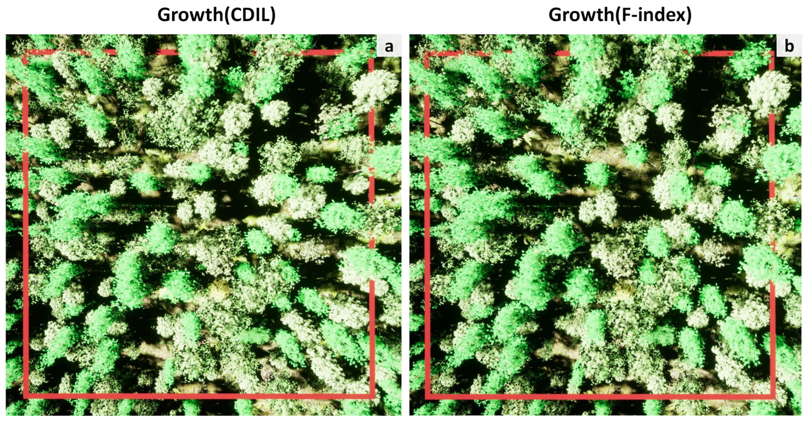
3.3. Adjustment of the Stand Spatial Structure after Logging

We used ArcMap software to obtain weighted Delaunay and Voronoi diagrams. The distance and the angle between the target tree and its nearest four trees were calculated in the attribute table. We used relevant formulas to calculate the average U-index, PV-index, M-index, and W-index of the five plots under the nonharvesting scenario and obtained the 10%, 20%, and 30% thinning intensities in the Unreal Engine 4 blueprint function.

Table 5. Comparison of spatial structure parameters of different thinning intensities in different plots.

Plots	Parameters	Intensity/0%	Intensity/10%	Intensity/20%	Intensity/30%
a	$\stackrel{-}{M}$	0.663	0.692	0.718	0.733
	$\stackrel{-}{W}$	0.521	0.489	0.480	0.472
	$\stackrel{-}{U}$	0.511	0.497	0.496	0.5
	${PV}_i$	1.919	1.855	1.908	1.903
b	$\stackrel{-}{M}$	0.635	0.679	0.702	0.725
	$\stackrel{-}{W}$	0.519	0.494	0.479	0.477
	$\stackrel{-}{U}$	0.521	0.51	0.503	0.501
	${PV}_i$	1.607	1.647	1.619	1.605
c	$\stackrel{-}{M}$	0.694	0.728	0.729	0.739
	$\stackrel{-}{W}$	0.547	0.503	0.488	0.469
	$\stackrel{-}{U}$	0.502	0.484	0.49	0.489
	${PV}_i$	1.805	1.791	1.746	1.718
d	$\stackrel{-}{M}$	0.719	0.735	0.724	0.726
	$\stackrel{-}{W}$	0.522	0.475	0.478	0.447
	$\stackrel{-}{U}$	0.506	0.482	0.492	0.484
	${PV}_i$	1.797	1.706	1.675	1.612
e	$\stackrel{-}{M}$	0.532	0.576	0.617	0.661
	$\stackrel{-}{W}$	0.518	0.519	0.496	0.475
	$\stackrel{-}{U}$	0.488	0.476	0.491	0.484
	${PV}_i$	1.571	1.567	1.563	1.604

shows the spatial structure parameters of different thinning intensities in different plots.

After logging, the average U-index of the five plots was close to 0.5, indicating that there was no significant difference in the size of the trees after management. The stands were in the middle state as per the quantitative index of the stand distribution state proposed by Hui Gangying [2]. The results showed that the average W-index of the stands in each plot was between 0.475 and 0.517 when the thinning intensity was 20%. The distribution of each plot gradually changed from aggregated distribution to random distribution. The variables of the average M-index of the five plots increased their thinning intensity. The average M-index of the stands in each plot was between 0.5 and 0.75, which belonged to medium-intensity mixing. The average PV-indexes of Plots a, c, and d gradually decreased with increasing thinning intensity. This was because the larger the PV-index, the more densely were the target trees covered, and the smaller the PV value, the better the stand adjustment effect. When the thinning intensity of Plot b was 30%, the value of the PV-index was lower than the original value. When the thinning intensities of Plot e were 20% and 30%, the value of the PV-index decreased compared with the original value, indicating that the PV-index reduced the degree to which the target tree was covered. The spatial structure parameters of all plots reached the optimal value when the thinning intensity was 20%, the exception being Plot e. Therefore, the optimal thinning intensity of the five plots was 20%, which was more conducive to adjusting the stand structure.

3.4. Interactive Visual Simulation of Forest Management

According to the measured data of each tree and the morphological structure data, the 3D models of 19 kinds of trees, such as Cunninghamia lanceolate, Schima Superba, and Machilus pauhoi Kaneh were built using by SpeedTree software. The 3D models of trees were added to the 3D scene as a class, and we read the coordinates in the stands data table of the plot through the inaccurate transform longitude latitude height to the unreal node under the CesiumGeoreference reference in the UE4 3D rendering engine. According to the scaling ratio calculated by the trunk and crown grading model, we loaded the trees in each plot according to the location. Figure 4 shows the simulation results of the initial stand scenarios of the five plots.

The 2D point data representing the distribution of trees could reflect the characteristics of single trees, such as the crown, the diameter at breast height, the tree height, and the crowding degree (Figure 5). However, these data were incomplete. On the other hand, the trees displayed in the 3D scene using 3D visual simulation technology helped not only directly observe the compression between tree crowns, the size difference, the spatial distribution pattern of trees, and the diversity of tree species, it also dynamically expressed the whole cutting and tending process (Figure 4), offering obvious advantages in analyzing, adjusting, and harvesting the stand structure.

To calculate the spatial structure parameters of each tree and each parameter index of the tree by the UE4 blueprint function script, a set of methods were developed. On the basis of the eight spatial structure parameters, the CDIL was calculated in real time in UE4 and a table providing information on the trees for harvest was generated. The system automatically logged according to the information table and the implemented growth simulation. Considering that the spatial structure of the stand would change in real time during the process of thinning and growth, the whole management simulation process would change dynamically in real time according to the management operation. Taking Plot c as an example, panels 1–3 in Figure 6 show that most of the trees selected for harvest by the CDIL were distributed in densely forested areas. With the naked eye, we could directly see from the top that the harvest trees were mainly trees with a small crown and poor growth, following the principle of cutting trees in dense areas and retaining trees in sparse areas. However, panels 4–6 in Figure 6 show that most of the trees selected for harvest by the F index were distributed in the areas with sparse trees, and the crowns of the trees identified for harvest tree were relatively large, which did not conform to the principle of cutting the small trees and retaining the large one. Studies by, for example, Li et al. [22], Pérezdelis et al. [44], and Lv et al. [29] have achieved good results in the research on the adjustment of the stand spatial structure, however, the accuracy of the results was reflected only by the parameter calculation, they lacked the visual expression of the simulation results from a 3D perspective (Figure 6).

Furthermore, panels 1–3 in Figure 7 represent the stand state after management by the CDIL, indicating that many trees with a small crown covered by adjacent trees were cut. The spatial distribution pattern of Plot c was changed from aggregate distribution to random distribution, which improved the diversity of tree species and the stability of the stand. Additionally, panels 4–6 in Figure 7 represented the stand state after management by the F index, from which we can intuitively see that many trees with large crowns were cut. The number of tree species in the stand decreased significantly after cutting, which violated the adjustment principle of improving the diversity of tree species. These results show that the CDIL gave a more reasonable selection of trees for harvest than the F index.

According to the growth model of each tree species, the growth of the stand was simulated. No.1 in Figure 8 represents the growth with a 20% thinning intensity by the CDIL, and No.2 in Figure 8 represents the growth after a 20% thinning intensity by the F index. The stand growth state after adjustment of the stand spatial structure can be seen.

3.5. Evaluation of the Stand Adjustment Effect

Forest management generally focuses on the analysis of the stand status, generally reflected in space utilization, species diversity, competition of constructive species, and stand composition. Therefore, this study analyzed and evaluated the effect of stand structure adjustment before and after stand management from seven aspects: the C-index, the H-index, the D-index, the B-index, the M-index, the PV-index, and the CDIL. The logging index constructed by Lv et al. was calculated and applied to this study for comparison.

Table 6. Changes in stand spatial structure parameters before and after 20% thinning.

Plots	Management 1	H-Index	C-Index	D-Index	B-Index	W-Index	M-Index	PV-Index	CDIL	Fi 2
a	Before management	0.525	4.775	0.695	0.291	0.521	0.663	1.919	34.925	2.408
	After management	0.628	1.855	0.648	0.317	0.489	0.733	1.855	2.59	1.313
	Change range/%	19.6	61.2	6.8	8.9	6.1	10.6	3.3	92.6	45.4
b	Before management	0.517	2.193	0.686	0.315	0.519	0.635	1.607	23.583	2.054
	After management	0.6	1.929	0.652	0.331	0.494	0.725	1.647	2.671	1.306
	Change range/%	16.1	12	5	5.1	4.8	14.2	2.5	88.7	36.4
c	Before management	0.516	2.775	0.705	0.285	0.547	0.694	1.815	17.301	4.207
	After management	0.632	2.467	0.671	0.303	0.503	0.738	1.781	2.315	1.354
	Change range/%	22.5	11.1	4.8	6.3	8	6.3	1.9	86.7	67.8
d	Before management	0.524	2.369	0.654	0.35	0.522	0.719	1.797	9.357	3.094
	After management	0.65	1.682	0.617	0.367	0.475	0.726	1.706	1.414	1.416
	Change range/%	24	29	5.7	4.9	9	1	5.1	84.9	54.2
e	Before management	0.536	2.389	0.699	0.269	0.518	0.532	1.571	26.248	3.41
	After management	0.608	2.172	0.669	0.288	0.496	0.661	1.547	4.355	1.26
	Change range/%	13.4	9.1	4.3	7.1	4.2	24.2	1.5	83.4	63.1

Note: ¹ The relative changes in stand spatial structure parameters for all plots before and after 10% thinning. ² The composite spatial structure index proposed by Lv et al. [30].

presents the results of changes in stand structure parameters and the value of the F index constructed by Lv et al. before and after thinning in each plot.

After the application of the CDIL to the tending and cutting management of the five plots, the change range of the stand H-index was more than 10%, and the health status of the stand was better than that before the management. The PV-index of Plots a, c, d, and e decreased after management and varied from 1.919 to 1.855, 1.815 to 1.781, 1.797 to 1.706, and 1.571 to 1.547, respectively, indicating that the overall coverage of the stand was also decreasing. The PV-index of Plot b increased slightly, by 0.04. The M-indexes of the five plots after the management increased by 10.6%, 14.2%, 6.3%, 1%, and 24.2%, respectively, maintaining the diversity of the tree species in stands. The change in the C-index was also obvious after the management. From the results, the C-index of Plot a had the most obvious change, with a decline of 61.2%, followed by that of Plot d, with a decline of 29%, indicating that this management reduced the competitive pressure on trees and improved the competitiveness of trees. The B-indexes of all plots increased. The D-index decreased after the management, which improved the living space of trees and protected the stability of the forest structure.

The average CDIL in each plot changed by 92.6%, 88.7%, 86.7%, 84.9%, and 83.4%, respectively, after management, with an increase of more than 80%. The change in Plot a was the greatest, indicating that the management effect was the best. However, the values of the F index by Lv et al. of Plots a-e had changed by 45.4%, 36.4%, 67.8%, 54.2%, and 63.1% respectively. Different from the study by Lv et al., the CDIL adds the vertical spatial structure parameter based on the horizontal spatial structure parameters, which takes into consideration the phenomenon of adjacent trees covering the target trees. Therefore, after logging, the change range of the average CDIL of the stand was greater than that of the F index.

We normalized the average W-indexes, U-indexes, M-indexes, B-indexes, H-indexes, D-indexes, and C-indexes in the five plots of trees selected for harvest by the CDIL and the F index in Table 2. Then, we obtained the average of the normalized values of each indicator of the five plots. The result showed that the value of the trees selected for harvest by the CDIL was 0.703 and the value of the trees selected for harvest by the F index was 0.528, indicating that the CDIL method was 11.4% more accurate than the F index. These results show that under the same horizontal spatial structure parameters, considering the influence of vertical spatial structure parameters on trees made the identification of trees for harvest more reasonable and accurate.

4. Discussion

In the forest ecosystem, the interaction between trees is essential to controlling the competition status, health, living space, and crown formation of trees. Analyzing and adjusting the complex forest structure can improve the biodiversity and stability of the forest. Therefore, reasonable thinning is the key factor in improving the stand structure and adjusting the stand density. We should consider the influence of horizontal and vertical parameters on the stand spatial structure. In this study, we selected eight spatial structure parameters and successfully constructed a comprehensive decision index of logging. On the basis of the UE4 3D rendering engine, according to the calculation results of the CDIL, the data table of harvest trees in each plot was established and management logging of 10%, 20%, and 30% intensities was simulated. The changes in stand structure indexes before and after management under different thinning intensities were compared and analyzed. The results indicated that the CDIL could effectively and reasonably select trees in the stand for harvest, making the adjusted forest structure stable and healthy.

4.1. Dynamic Changes in Stand Structure Parameters

To express dynamic changes in stand structure characters, we used eight parameters to describe subtler features of each tree: W-index, U-index, PV-index, H-index, B-Index, D-index, M-index, and C-index.

The W-index was used to analyze the individual distribution pattern of the trees in a forest and can be used to reconstruct complex forest structures [40,45]. To date, many scholars studying neighborhood patterns have shown that the distribution pattern of most trees is random [41,46]. In this study, the average W-index for all of the plots before logging was higher than 0.517, indicating aggregate distribution. However, after the implementation of the 20% thinning intensity measure, the average W-index of the stand in each plot was between 0.475 and 0.517, indicating a gradual change from aggregate to random distribution [2,22]. This is similar to the results of previous research [40,45]. Our study showed that this management can increase the proportion of the random distribution of trees.

The U-index represents the spatial dominance of tree species [2,42]. In this study, the average U-index for all plots was closer to 0.5 after cutting than before cutting, indicating that the size of trees was uniform after management and the stand was in the middle state. These results are the same as the findings of other studies [44,47].

The average M-indexes for all plots increased after logging. The greater the M-index, the higher the diversity of tree species [3,44,48]. Therefore, the M-index was beneficial to the growth and diversity of trees.

PV indicates the degree of influence of tree cover in the vertical direction. The smaller the PV-index, the less the trees are covered and the better the trees grow [32]. In this study, The PV-index for all plots decreased with the increase in the thinning intensity and the best effect was achieved when the thinning intensity was 20%. This result shows that the effect of the PV-index on the stand structure was effective, which was not found in other studies [17,25,29].

The H-index and the B-index represent the health status of trees and the openness of stands. The H-indexes and B-indexes for all plots increased after the trees were cut, indicating that the H-index and the B-index increased the growth and development space of the trees. The health status of the stands improved.

The C-index and the D-index represent the competitiveness of the trees and the degree of crowding of stands [37]. In this study, the values of the C-index and the D-index for all plots changed greatly after logging, especially the values of the C-index, which showed that management reduced the competitive pressure on trees and improved their competitiveness.

The above eight indicators considered the characteristics of trees in the horizontal and vertical structural directions respectively. As per our results, the optimal thinning intensity of the five plots was 20%, which was more conducive to adjusting the stand structure. The thinning intensity mainly concentrated on the trees with a high aggregation, poor health, low mingling, and a high competition status. However, different optimization objectives led to different optimal intensities [44,49]. Therefore, more research is needed to explore the optimal thinning intensity that affects all aspects of the ecosystem.

4.2. Evaluation of the CDIL

In this study, the index that had the largest impact on the CDIL was the C-index. The correlation between the PV-index and the CDIL was 0.61, ranking fourth in terms of correlation. The CDIL in the five plots decreased by 92.6%, 88.7%, 86.7%, 84.9%, and 83.4%, respectively. Different from the cutting index proposed by Gadow et al. [24], Li et al. [22], and Lv et al. [29], which only considered some stand structure characteristics of trees, the comprehensive decision index of logging proposed in this paper selected eight indexes that influence the horizontal and vertical structure of trees. The simulation results showed that with an increase in the thinning intensity, the CDIL values for all plots were significantly reduced. The change range of the eight stand structure parameters before and after management showed that thinning could increase the dominance, openness, stability, and mixing degree of trees and reduce the competitive pressure and density of the target trees. These results are consistent with those of other research [11,22,24]. Taking Plot c as an example, the PV-index of the stand in Plot c decreased from 1.815 before management to 1.781 afterward, indicating that the degree of coverage above the trees was greatly reduced after management. It not only considered the vertical distribution of trees, it also improved the growth space of trees. In addition, in Plot c, the CDIL index was 17.301 before management and 2.315 after management, with a change of 14.986, and a decrease of about 7.5 times. These results show that the CDIL could reasonably and accurately select trees for harvest and improve the stability of the stand structure.

This form of management greatly reduced the competitive pressure on the top tree species and improved the competitive ability and tree species advantage of the top tree species. The degree of crowding in the forest was reduced, the living space of the forest was improved, and the stability of the forest structure was maintained. Compared with the harvesting index constructed by other scholars, our index was advantageous in that it comprehensively considered the impact of horizontal and vertical directions on spatial structure and used eight horizontal and vertical spatial structure parameters. A comparison with the index constructed by Lv et al. shows that the CDIL was 11.4% more accurate than the F index in selecting harvest trees. The real process of cutting management and growth simulation was simulated in the UE4 engine by using visualization techniques. Compared with the 2D results of other scholars’ studies [22,29,42], the simulation in this paper enabled managers to observe the change process of the stand spatial structure more accurately.

The CDIL has proven to be accurate and reasonable for comprehensively considering horizontal and vertical spatial structure parameters to make stand structure adjustment more effective. It is easy to use and less dependent on experience. It can greatly improve the growth and development space of trees. However, the application of CDIL to other types of forests and landscapes is still restricted due to numerous reasons, such as the limited plot number and tree number, and the fact that climatic conditions and topographic factors are not considered. Moreover, the CDIL considers the spatial structure characteristics of trees and does not consider the collision and extrusion between tree crowns or reflect them in the virtual scene. In the next research, the collision and extrusion between tree crowns will be added to the index as a factor and will be presented in a visual way.

5. Conclusions

In this study, we constructed a highly efficient, objective, and accurate comprehensive decision index of logging (CDIL) by combining the quantitative indicators representing the health status, density, distribution pattern, and competition status of the stands and used them to select trees for harvest. The results of the stand spatial structure adjustment of the index under different thinning intensities show that the optimum thinning intensity was 20%. The numbers of trees to be cut in the five sample plots were 43, 43, 44, 40, and 45 and these were mainly distributed in areas with an uneven forest size and dense forest size differentiation. After stand adjustment, the average CDIL in each plot decreased by more than 90%. The average W-index of the stand improved from 0.475 to 0.517, showing a gradual change from aggregate distribution to random distribution. This showed that the CDIL application effectively adjusts the spatial structure of the stand and makes the stand structure more stable. The CDIL index was compared with the F index constructed by Lv et al., and the results show that the CDIL was 11.4% more accurate than the F index in identifying trees for harvest. The visual simulation technology was closely combined with tending and felling and displayed the entire process of actual forest tending and felling, which will enable forest managers to observe the structural characteristics of forests more intuitively and formulate forest management plans in time. However, to make the selection of logging more accurate, we will consider the impact of crown extrusion in the future.

References

1. Zhang, L.; Hui, G.; Hu, Y.; Zhao, Z. Spatial structural characteristics of forests dominated by Pinus tabulaeformis Carr. PLoS ONE 2018, 13, e0194710. [Google Scholar] [CrossRef] [Green Version]
2. Hui, G.; Zhang, G.; Zhao, Z.; Yang, A. Methods of forest structure research: A review. Curr. For. Rep. 2019, 5, 142–154. [Google Scholar] [CrossRef]
3. Wan, P.; Zhang, G.; Wang, H.; Zhao, Z.; Hu, Y.; Zhang, G.; Hui, G.; Liu, W. Impacts of different forest management methods on the stand spatial structure of a natural Quercus aliena var. acuteserrata forest in Xiaolongshan, China. Ecol. Inform. 2019, 50, 86–94. [Google Scholar] [CrossRef]
4. Kerr, G. The use of silvicultural systems to enhance the biological diversity of plantation forests in Britain. For. An Int. J. For. Res. 1999, 72, 191–205. [Google Scholar] [CrossRef] [Green Version]
5. Hanewinkel, M.; Pretzsch, H. Modelling the conversion from even-aged to uneven-aged stands of Norway spruce (Picea abies L. Karst.) with a distance-dependent growth simulator. For. Ecol. Manage. 2000, 134, 55–70. [Google Scholar] [CrossRef]
6. Mickaël, H.; Michaël, A.; Fabrice, B.; Pierre, M.; Thibaud, D. Soil detritivore macro-invertebrate assemblages throughout a managed beech rotation. Ann. For. Sci. 2007, 64, 219–228. [Google Scholar] [CrossRef]
7. Aguirre, O.; Hui, G.Y.; von Gadow, K.; Javier, J. An analysis of spatial forest structure using neighbourhood-based variables. For. Ecol. Manag. 2003, 183, 137–145. [Google Scholar] [CrossRef]
8. Kint, V.; Meirvenne, M.; Nachtergale, L.; Geudens, G.; Lust, N. Spatial methods for quantifying forest stand structure development: A comparison between nearest-neighbor indices and variogram analysis. For. Sci. 2003, 49, 36–49. [Google Scholar] [CrossRef]
9. Antos, J.A.; Parish, R. Dynamics of an old-growth, fire-initiated, subalpine forest in southern interior British Columbia: Tree size, age, and spatial structure. Can. J. For. Res. 2002, 32, 1935–1946. [Google Scholar] [CrossRef]
10. North, M.; Chen, J.; Oakley, B.; Song, B.; Rudnicki, M.; Gray, A.; Innes, J. Forest stand structure and pattern of old-growth western hemlock/Douglas-fir and mixed-conifer forests. For. Sci. 2004, 50, 299–311. [Google Scholar] [CrossRef]
11. Li, Y.; Hui, G.; Ye, S.; Hui, G.; Hu, Y.; Zhao, Z. Spatial structure of timber harvested according to structure-based forest management. For. Ecol. Manag. 2014, 322, 106–116. [Google Scholar] [CrossRef]
12. Adams, D.M.; Latta, G.S. Effects of a forest health thinning program on land and timber values in eastern Oregon. J. For. 2004, 102, 9–13. [Google Scholar] [CrossRef]
13. Paletto, A.; Meo, I.D.; Grilli, G.; Nikodinoska, N. Effects of different thinning systems on the economic value of ecosystem services: A case-study in a black pine peri-urban forest in Central Italy. Ann. For. Res. 2017, 60, 313–326. [Google Scholar]
14. Forrester, D.I.; Elms, S.R.; Baker, T.G. Tree growth-competition relationships in thinned Eucalyptus plantations vary with stand structure and site quality. Eur. J. For. Res. 2013, 132, 241–252. [Google Scholar] [CrossRef]
15. Forrester, D.I. Linking forest growth with stand structure: Tree size inequality, tree growth or resource partitioning and the asymmetry of competition. For. Ecol. Manage. 2019, 447, 139–157. [Google Scholar] [CrossRef]
16. Pommerening, A. Evaluating structural indices by reversing forest structural analysis. For. Ecol. Manag. 2006, 224, 266–277. [Google Scholar] [CrossRef]
17. Darenova, E.; Crabbe, R.A.; Knott, R.; Uherková, B.; Kadavý, J. Effect of coppicing, thinning and throughfall reduction on soil water content and soil CO2 efflux in a sessile oak forest. Silva Fenn. 2018, 52, 9927. [Google Scholar] [CrossRef] [Green Version]
18. Hill, M.; Pospíšil, M. On the relation between the secretion of the perivascular mast cells and the serum level of mucoproteins. Experientia 1959, 15, 267–269. [Google Scholar] [CrossRef]
19. Johnson, D.W.; Murphy, J.D.; Walker, R.F.; Miller, W.W.; Glass, D.W.; Todd, D.E. The combined effects of thinning and prescribed fire on carbon and nutrient budgets in a Jeffrey pine forest. Ann. For. Sci. 2008, 65, 601. [Google Scholar] [CrossRef] [Green Version]
20. Dong, L.; Wei, H.; Liu, Z. Optimizing forest spatial structure with neighborhood-based indices: Four case studies from northeast China. Forests 2020, 11, 413. [Google Scholar] [CrossRef] [Green Version]
21. Ye, S.X.; Zheng, Z.R.; Diao, Z.Y.; Ding, G.D.; Bao, Y.F.; Liu, Y.D.; Gao, G.L. Effects of thinning on the spatial structure of Larix principis-rupprechtii plantation. Sustainability 2018, 10, 1250. [Google Scholar] [CrossRef]
22. Li, Y.; Hui, G.Y.; Wang, H.X.; Zhang, L.J.; Ye, S.X. Selection priority for harvested trees according to stand structural indices. iForest 2017, 10, 561–566. [Google Scholar] [CrossRef] [Green Version]
23. Von Gadow, K.; Hui, G.Y. Modelling forest development. For. Sci. 1999, 57, 46–58. [Google Scholar]
24. Von Gadow, K.; Zhang, C.; Wehenkel, C.; Pommerening, A.; Corral-Rivas, J.; Korol, M.; Myklush, S.; Hui, G.Y.; Kiviste, A.; Zhao, X.H. Forest Structure and Diversity; Springer: Berlin, Germany, 2012; pp. 30–62. [Google Scholar]
25. Song, Y.F. Individual Tree Growth Models and Competitors Harvesting Simulation for Target Tree-Oriented Management. Ph.D. Thesis, Chinese Academy of Forestry, Beijing, China, 2015. (In Chinese). [Google Scholar]
26. Pastorella, F.; Paletto, A. Stand Structure Indices as Tools to Support Forest Management: An Application in Trentino Forests (Italy). J. For. Sci. 2013, 59, 159–168. [Google Scholar] [CrossRef] [Green Version]
27. Courbaud, B.; Goreaud, F.; Dreyfus, P.; Bonnet, F.R. Evaluating thinning strategies using a tree distance dependent growth model: Some examples based on the CAPSIS software “uneven-aged spruce forests” module. For. Ecol. Manage. 2001, 145, 15–28. [Google Scholar] [CrossRef]
28. Cao, X.Y.; Li, J.P.; Hu, Y.J.; Yang, J. Spatial structure optimizing model of stand thinning of Cunninghamia lanceolata ecological forest. J. Chin. J. Ecol. 2017, 36, 1134–1141. (In Chinese) [Google Scholar]
29. Lv, Z.S.; Liu, Z.G.; Dong, L.B.; Zhang, L.Y.; Sun, Y.X. Simulation of Mixed Forest Structure Optimization with Comprehensive Cutting Index in Maoer Mountain. J. Northeast. For. Univ. 2018, 46, 12–17. (In Chinese) [Google Scholar]
30. Ahmad, B.; Wang, Y.; Hao, J.; Liu, Y.; Bohnett, E.; Zhang, K. Optimizing Stand Structure for Tradeoffs between Overstory and Understory Vegetation Biomass in a Larch Plantation of Liupan Mountains, Northwest China. For. Ecol. Manage. 2019, 443, 43–50. [Google Scholar] [CrossRef]
31. Bhandari, S.K.; Veneklaas, E.J.; McCaw, L.; Mazanec, R.; Whitford, K.; Renton, M. Individual Tree Growth in Jarrah (Eucalyptus marginata) Forest Is Explained by Size and Distance of Neighbouring Trees in Thinned and Non-Thinned Plots. For. Ecol. Manage. 2021, 494, 119364. [Google Scholar] [CrossRef]
32. Li, S.J.; Zhang, H.Q.; Li, Y.L.; Yang, T.D.; He, J.P.; Ma, Z.Y.; Seng, K. Dynamic Visual Simulation of Chinese Fir Stand Growth Based on Sample Library. J. For. Res. 2019, 32, 21–30. (In Chinese) [Google Scholar]
33. Pommerening, A. Approaches to Quantifying Forest Structures. For. An Int. J. For. Res. 2002, 75, 305–324. [Google Scholar] [CrossRef]
34. Hui, G.Y.; Gadow, K.V.; Albert, M. The neighborhood pattern-a new structure parameter for describing distribution of forest tree position. Sci. Silvae Sin. 1999, 35, 37–42. (In Chinese) [Google Scholar]
35. Hui, G.Y.; Gadow, K.V.; ALbert, M. A New Parameter for Stand Spatial Structure—Neighbourhood Comparison. J. For. Res. 1999, 12, 1–6. [Google Scholar]
36. Tanaka, K.; Tokuda, M. Negative correlation between dispersal investment and canopy openness among populations of the ant-dispersed sedge, Carex lanceolata. Plant Ecol. 2020, 221, 1105–1115. [Google Scholar] [CrossRef]
37. Hegyi, F. A simulation model for managing jack-pine stands. In Growth Models for Tree and Stand Simulation; Fries, J., Ed.; IUFRO: Vienna, Austria, 1974; pp. 74–90. [Google Scholar]
38. Hui, G.; Zhao, X.; Zhao, Z.; Gadow, K. Evaluating tree species spatial diversity based on neighborhood relationships. For. Sci. 2011, 57, 292–300. [Google Scholar] [CrossRef]
39. Zeng, Q.Y.; Zhou, Y.M.; Li, J.P.; Liu, S.Q. Decision-making Methodology of Forest Ecosystem Management Based on Spatial Structure Factors of Forest. J. Northeast. For. Univ. 2010, 38, 31–35. (In Chinese) [Google Scholar]
40. Li, Y.; Hui, G.; Zhao, Z.; Hu, Y. The bivariate distribution characteristics of spatial structure in natural Korean pine broad-leaved forest. J. Veg. Sci. 2012, 23, 1180–1190. [Google Scholar] [CrossRef]
41. Li, Y.; He, J.; Yu, S.; Wang, H.; Ye, S. Spatial structures of different-sized tree species in a secondary forest in the early succession stage. Eur. J. For. Res. 2020, 139, 709–719. [Google Scholar] [CrossRef]
42. Cao, X.; Li, J.; Feng, Y.; Hu, Y.; Zhang, C.; Fang, X.; Deng, C. Analysis and evaluation of the stand spatial structure of Cunninghamia lanceolata ecological forest. Sci. Silvae Sin. 2015, 51, 37–48. [Google Scholar]
43. Azzeh, M.; Neagu, D.; Cowling, P.I. Fuzzy Grey Relational Analysis for Software Effort Estimation; Kluwer Academic Publishers: Alphen am Rhein, The Netherlands, 2010. [Google Scholar]
44. Pérezdelis, G.; Garcíagonzález, I.; Rozas, V.; Arevalo, J.R. Effects of thinning intensity on radial growth patterns and temperature sensitivity in Pinus canariensis afforestations on Tenerife Island, Spain. Ann. For. Sci. 2011, 68, 1093–1104. [Google Scholar] [CrossRef] [Green Version]
45. Zhao, Z.; Hui, G.; Hu, Y.; Wang, H.; Zhang, G.; Gadow, K. Testing the significance of different tree spatial distribution patterns based on the uniform angle index. Can. J. For. Res. 2014, 44, 1417–1425. [Google Scholar] [CrossRef]
46. Zhang, G.; Hui, G.; Zhao, Z.; Hu, Y.; Wang, H.; Liu, W.; Zang, R. Composition of basal area in natural forests based on the uniform angle index. Ecol. Inf. 2018, 45, 1–8. [Google Scholar] [CrossRef]
47. Fang, X.; Tan, W.; Gao, X.; Chai, Z. Close-to-nature management positively improves the spatial structure of Masson pine forest stands. Web. Ecol. 2021, 21, 45–54. [Google Scholar] [CrossRef]
48. Zhao, Z.; Hui, G.; Hu, Y.; Li, Y.; Wang, H. Method and application of stand spatial advantage degree based on the neighborhood comparison. J. Beijing For. Univ. 2014, 36, 78–82. [Google Scholar]
49. Settineri, G.; Mallamaci, C.; Mitrović, M.; Sidari, M.; Muscolo, A. Effects of different thinning intensities on soil carbon storage in Pinus laricio forest of Apennine South Italy. Eur. J. For. Res. 2018, 137, 131–141. [Google Scholar] [CrossRef]
Figure 1. (A) Jiangxi Province. (B) Fenyi County. (C) Shanxia Experimental Forest Farm. (D) The distribution of trees in the five plots. Yellow squares represent the locations and sizes of the plots; the red lines represent the subplot boundaries; and graphs (ae) represent the distribution of trees in each plot respectively.
Forests 14 00277 g001
Figure 2. The construction process of the CDIL.
Forests 14 00277 g002
Figure 3. (A) represents the texture of Cunninghamia lanceolata bark. (B) represents the texture of Cunninghamia lanceolata leaves. (C) is the initial three-dimensional model and stump model of Cunninghamia lanceolata created by using (A,B), and real measurement data.
Forests 14 00277 g003
Figure 4. (A) The result of visual simulation of the five sample plots in the virtual scene. (B) The distribution result of the five sample plots; graphs (ae) represent the real position distribution of all the trees in each plot in the virtual scene.
Forests 14 00277 g004
Figure 5. Two-dimensional distribution of tree position. The green dots represent the location of trees; graphs (ae) represent the distribution of trees in each plot respectively.
Forests 14 00277 g005
Figure 6. Visual simulation of Plot c by the CDIL and the F index. (ac) The distribution of harvest trees identified by the CDIL. (df) The distribution of harvest trees identified by the F index. The red dots show logged trees.
Forests 14 00277 g006
Figure 7. Visual simulation of Plot c by the CDIL and the F index. (ac) The adjusted stand state by the CDIL. (df) The adjusted stand state by the F index.
Forests 14 00277 g007
Figure 8. Growth simulation of Plot c after thinning. with (a) representing the growth with a 20% thinning intensity by the CDIL and (b) representing the growth with a 20% thinning intensity by the F index.
Forests 14 00277 g008