

Informing Sustainable Forest Management: Remote Sensing Strategies for Assessing Soil Disturbance after Wildfire and Salvage Logging


 ,
,
Abstract
:1. Introduction
2. Materials and Methods
2.1. Fire Information
2.2. Field Sites
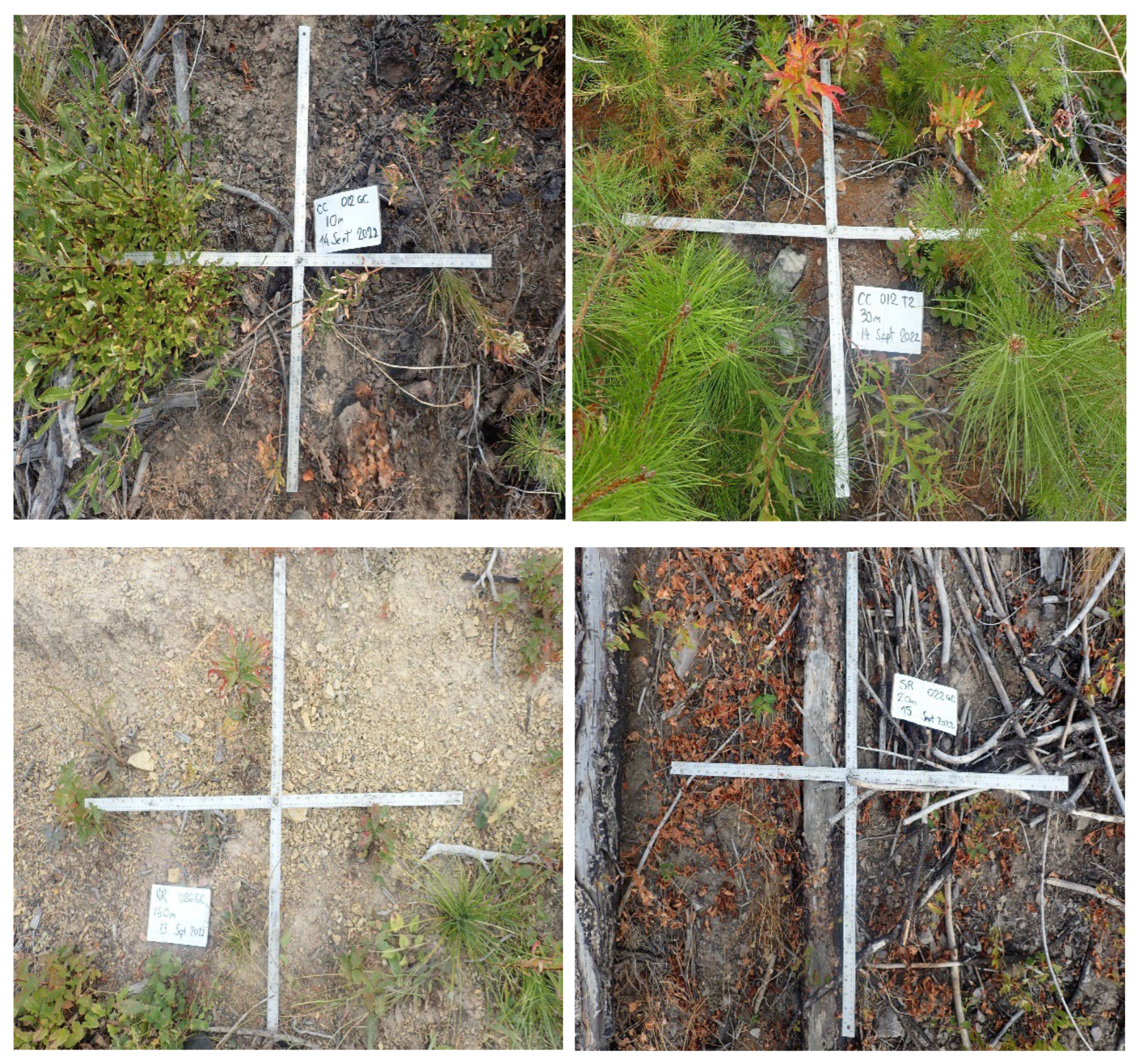
2.3. Field Sampling
2.4. Spatial Data Layers
2.5. Remotely Sensed Imagery
2.6. Statistics and Data Analysis
2.6.1. Overview
2.6.2. Model Details
3. Results
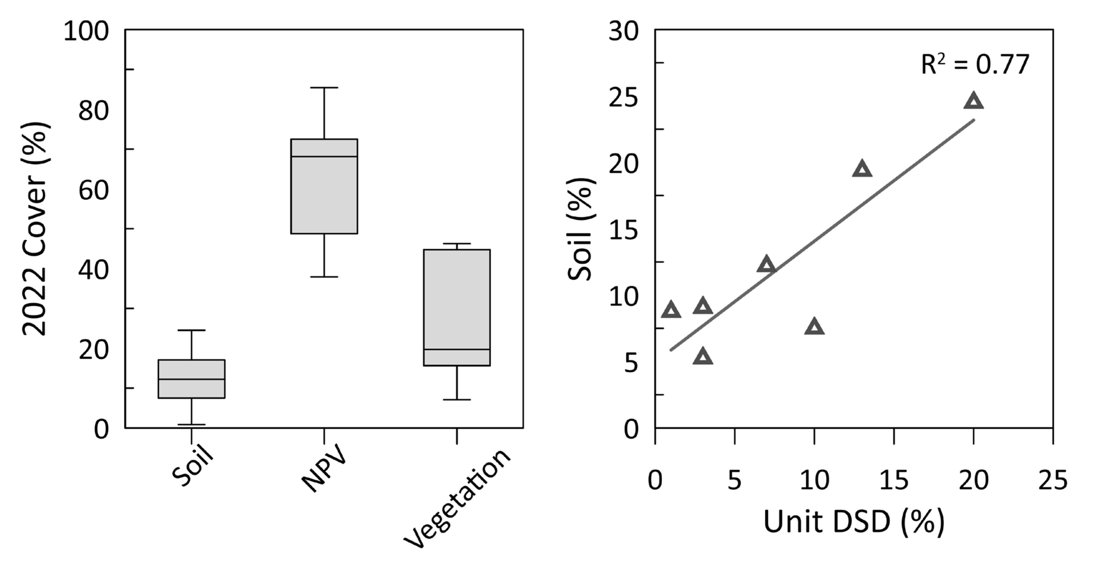
3.1. Ground Cover
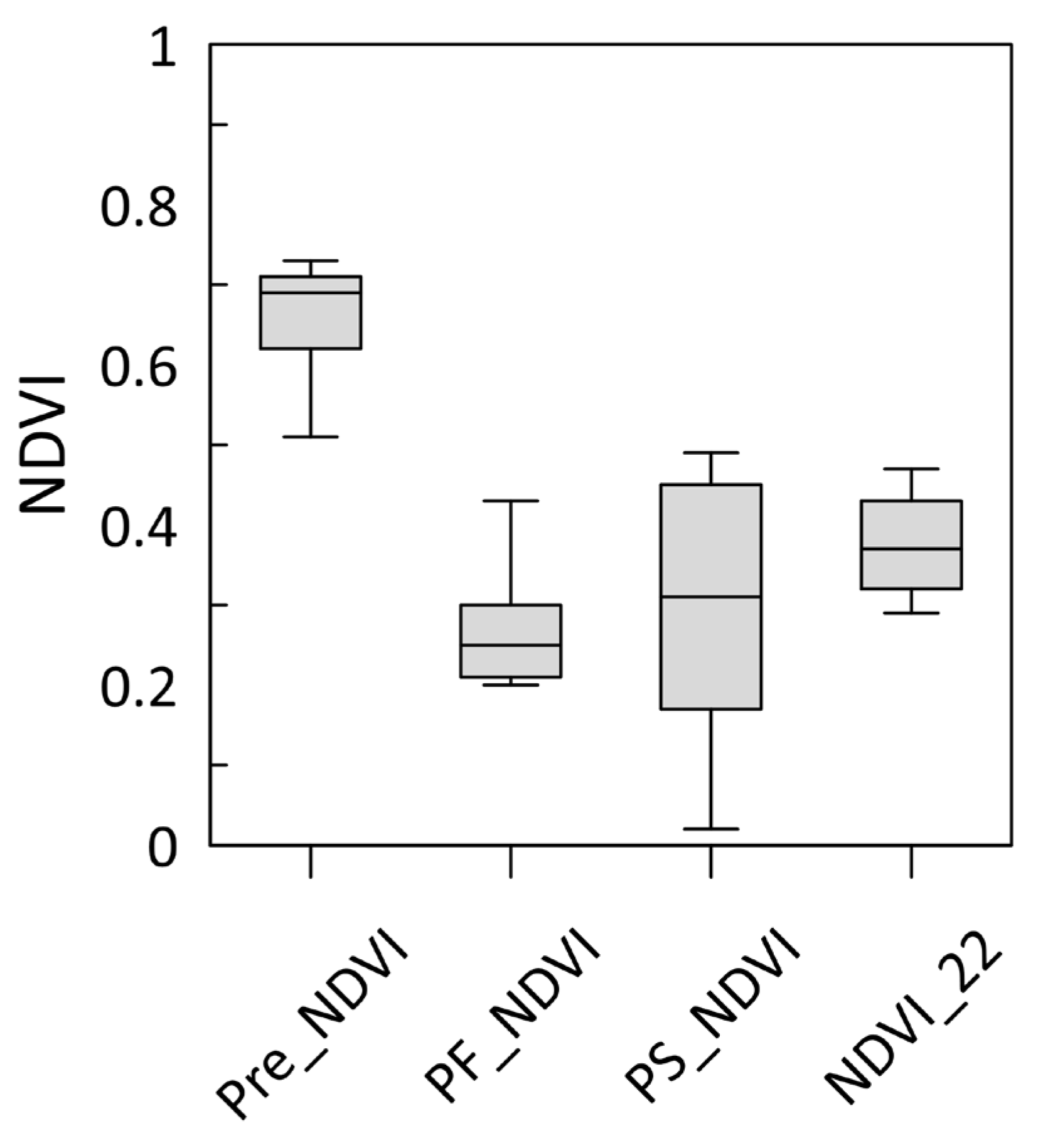
3.2. Imagery
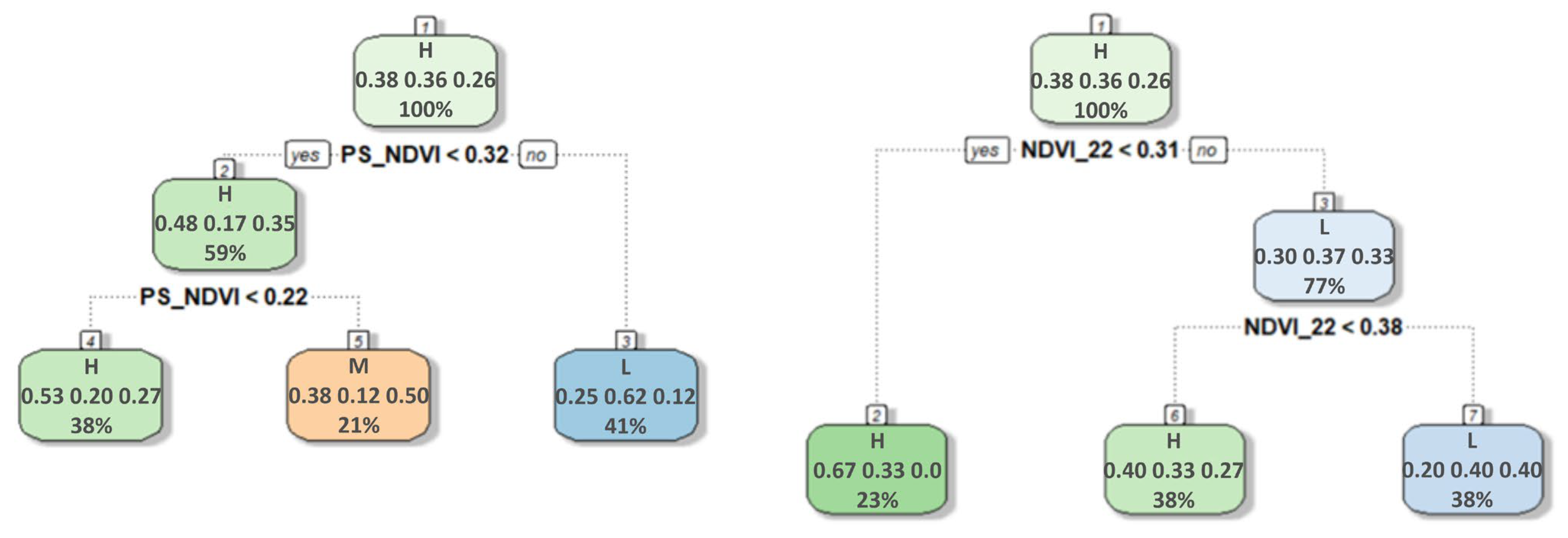
3.3. Classification
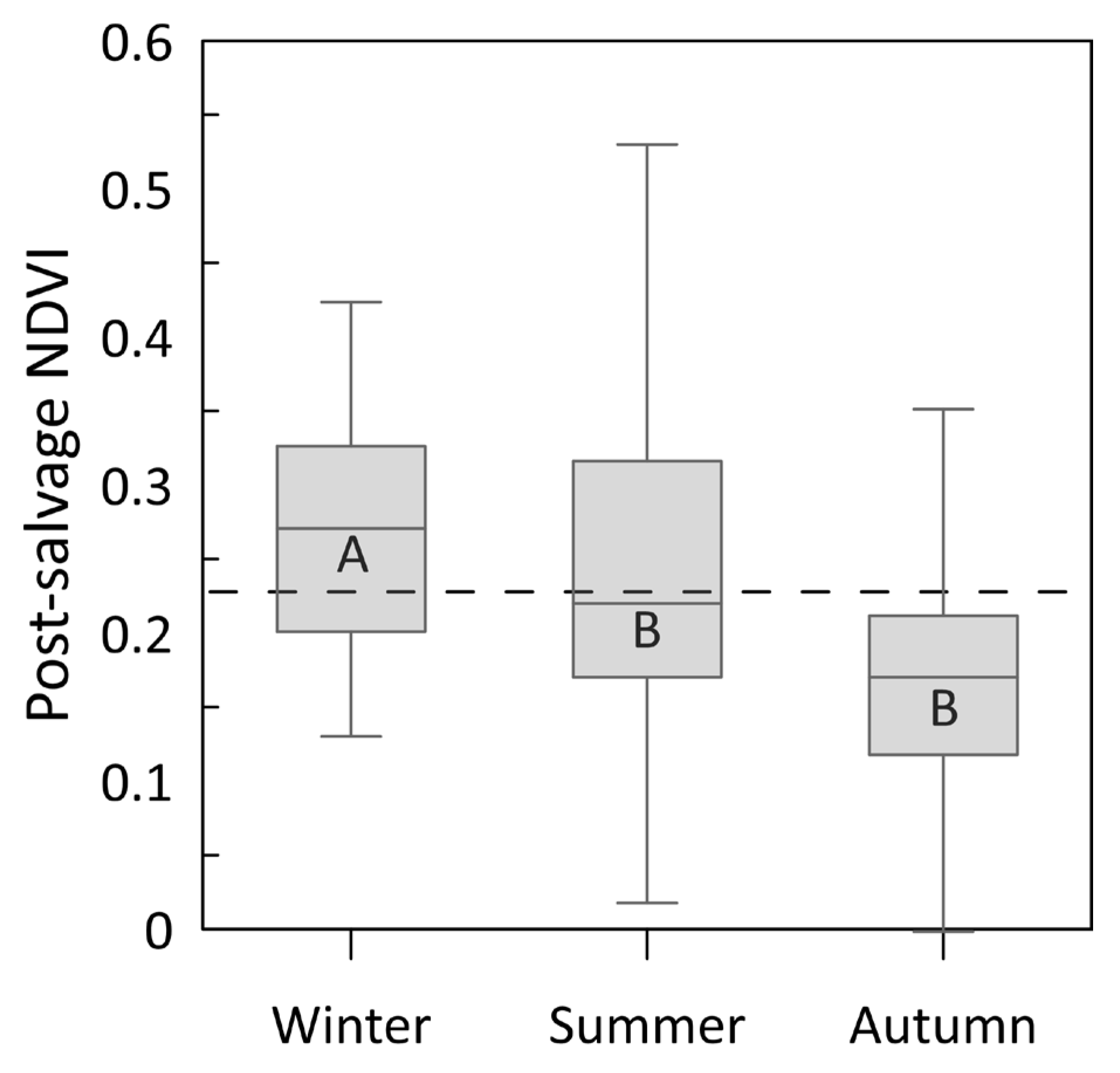
3.4. Mixed-Model Results
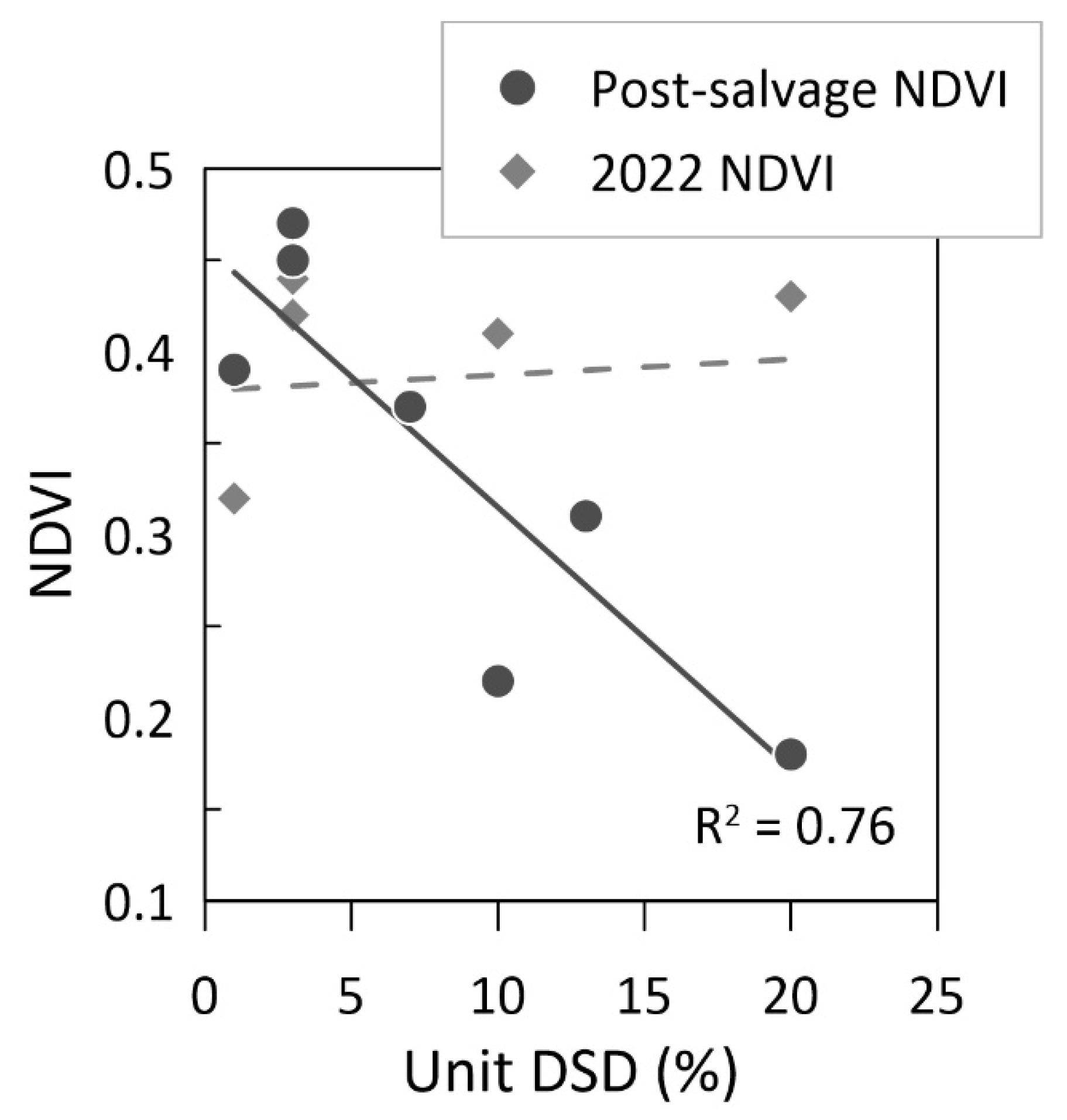
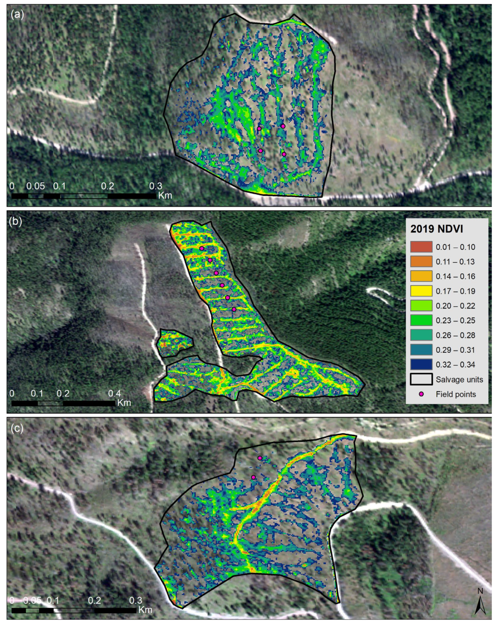
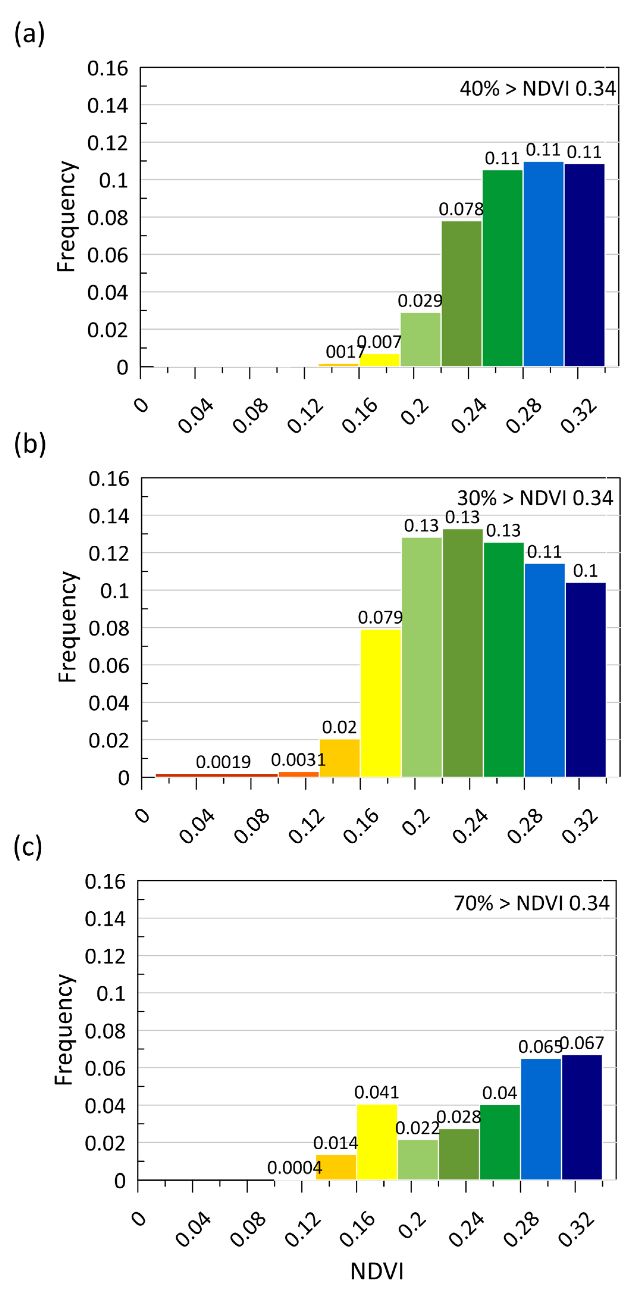
3.5. Imagery
4. Discussion
4.1. Ground Cover and DSD
4.2. Using Imagery to Map DSD
4.3. Management Considerations
5. Conclusions
Author Contributions
Funding
Data Availability Statement
Acknowledgments
Conflicts of Interest
References
- Abatzoglou, J.T.; Williams, A.P. Impact of Anthropogenic Climate Change on Wildfire across Western US Forests. Proc. Natl. Acad. Sci. USA 2016, 113, 11770–11775. [Google Scholar] [CrossRef] [PubMed]
- Stevens-Rumann, C.S.; Morgan, P. Tree Regeneration Following Wildfires in the Western US: A Review. Fire Ecol. 2019, 15, 15. [Google Scholar] [CrossRef]
- Westerling, A.L.; Hidalgo, H.G.; Cayan, D.R.; Swetnam, T.W. Warming and Earlier Spring Increase Western U.S. Forest Wildfire Activity. Science 2006, 313, 940–943. [Google Scholar] [CrossRef] [PubMed]
- Dennison, P.E.; Brewer, S.C.; Arnold, J.D.; Moritz, M.A. Large Wildfire Trends in the Western United States, 1984–2011. Geophys. Res. Lett. 2014, 41, 6413–6419. [Google Scholar] [CrossRef]
- Pausas, J.G.; Keeley, J.E. Wildfires as an Ecosystem Service. Front. Ecol. Environ. 2019, 17, 289–295. [Google Scholar] [CrossRef]
- Sessions, J.; Bettinger, P.; Buckman, R.; Newton, M.; Hamann, J. Hastening the Return of Complex Forests Following Fire: The Consequences of Delay. J. For. 2004, 102, 38–45. [Google Scholar]
- Thompson, M.P.; Calkin, D.E.; Finney, M.A.; Ager, A.A.; Gilbertson-Day, J.W. Integrated National-Scale Assessment of Wildfire Risk to Human and Ecological Values. Stoch. Environ. Res. Risk Assess. 2011, 25, 761–780. [Google Scholar] [CrossRef]
- Lentile, L.B.; Holden, Z.A.; Smith, A.M.S.; Falkowski, M.J.; Hudak, A.T.; Morgan, P.; Lewis, S.A.; Gessler, P.E.; Benson, N.C. Remote Sensing Techniques to Assess Active Fire Characteristics and Post-Fire Effects. Int. J. Wildland Fire 2006, 15, 319–345. [Google Scholar] [CrossRef]
- Parsons, A.; Robichaud, P.R.; Lewis, S.A.; Napper, C.; Clark, J.T. Field Guide for Mapping Post-Fire Soil Burn Severity; Gen. Tech. Rep. RMRS-GTR-243; US Department of Agriculture, Forest Service, Rocky Mountain Research Station: Fort Collins, CO, USA, 2010.
- Moody, J.A.; Shakesby, R.A.; Robichaud, P.R.; Cannon, S.H.; Martin, D.A. Current Research Issues Related to Post-Wildfire Runoff and Erosion Processes. Earth Sci. Rev. 2013, 122, 10–37. [Google Scholar] [CrossRef]
- Certini, G. Effects of Fire on Properties of Forest Soils: A Review. Oecologia 2005, 143, 1–10. [Google Scholar] [CrossRef]
- Neary, D.G.; Ryan, K.C.; DeBano, L.F. Wildland Fire in Ecosystems: Effects of Fire on Soils and Water; Gen. Tech. Rep. RMRS-GTR-42; US Department of Agriculture, Forest Service, Rocky Mountain Research Station: Ogden, UT, USA, 2005; Volume 4, pp. 1–250. [CrossRef]
- Olsen, W.H.; Wagenbrenner, J.W.; Robichaud, P.R. Factors Affecting Connectivity and Sediment Yields Following Wildfire and Post-Fire Salvage Logging in California’s Sierra Nevada. Hydrol. Process. 2021, 35, e13984. [Google Scholar] [CrossRef]
- Morgan, P.; Moy, M.; Droske, C.A.; Lewis, S.A.; Lentile, L.B.; Robichaud, P.R.; Hudak, A.T.; Williams, C.J. Vegetation Response to Burn Severity, Native Grass Seeding, and Salvage Logging. Fire Ecol. 2015, 11, 31–58. [Google Scholar] [CrossRef]
- Wienk, C.L.; Sieg, C.H.; McPherson, G.R. Evaluating the Role of Cutting Treatments, Fire and Soil Seed Banks in an Experimental Framework in Ponderosa Pine Forests of the Black Hills, South Dakota. For. Ecol. Manag. 2004, 192, 375–393. [Google Scholar] [CrossRef]
- Wagenbrenner, J.W.; Coe, D.B.R.; Olsen, W.H. Mitigating Potential Sediment Delivery from Post-Fire Salvage Logging. Calif. For. Rep. 2023, 7, 1–32. [Google Scholar]
- Powers, R.F.; Scott, D.A.; Sanchez, F.G.; Voldseth, R.A.; Page-Dumroese, D.; Elioff, J.D.; Stone, D.M. The North American Long-Term Soil Productivity Experiment: Findings from the First Decade of Research. For. Ecol. Manag. 2005, 220, 31–50. [Google Scholar] [CrossRef]
- Williams, C.J.; Pierson, F.B.; Robichaud, P.R.; Al-Hamdan, O.Z.; Boll, J.; Strand, E.K. Structural and Functional Connectivity as a Driver of Hillslope Erosion Following Disturbance. Int. J. Wildland Fire 2016, 25, 306–321. [Google Scholar] [CrossRef]
- Reeves, D.; Page-Dumroese, D.; Coleman, M. Detrimental Soil Disturbance Associated with Timber Harvest Systems on National Forests in the Northern Region; Res. Pap. RMRS-RP-89; US Department of Agriculture, Forest Service, Rocky Mountain Research Station: Fort Collins, CO, USA, 2011; pp. 1–12. [CrossRef]
- Wagenbrenner, J.W.; MacDonald, L.H.; Coats, R.N.; Robichaud, P.R.; Brown, R.E. Effects of Post-Fire Salvage Logging and a Skid Trail Treatment on Ground Cover, Soils, and Sediment Production in the Interior Western United States. For. Ecol. Manag. 2015, 335, 176–193. [Google Scholar] [CrossRef]
- Grigal, D.F. Effects of Extensive Forest Management on Soil Productivity. For. Ecol. Manag. 2000, 138, 167–185. [Google Scholar] [CrossRef]
- McIver, J.D.; Starr, L. A Literature Review on the Environmental Effects of Post-fire Logging. West. J. Appl. For. 2001, 16, 159–168. [Google Scholar] [CrossRef]
- Page-Dumroese, D.; Jurgensen, M.; Elliot, W.; Rice, T.; Nesser, J.; Collins, T.; Meurisse, R. Soil Quality Standards and Guidelines for Forest Sustainability in Northwestern North America. For. Ecol. Manag. 2000, 138, 445–462. [Google Scholar] [CrossRef]
- USDA. Forest Service National Forest Management Act (1976); USDA: Missoula, MT, USA, 1976.
- Reeves, D.A.; Reeves, M.C.; Abbott, A.M.; Page-Dumroese, D.S.; Coleman, M.D. A Detrimental Soil Disturbance Prediction Model for Ground-Based Timber Harvesting. Can. J. For. Res. 2012, 42, 821–830. [Google Scholar] [CrossRef]
- Naghidi, R.; Solgi, A.; Labelle, E.R.; Nikooy, M. Combined Effects of Soil Texture and Machine Operating Trail Gradient on Changes in Forest Soil Physical Properties during Ground-Based Skidding. Pedosphere 2020, 30, 508–516. [Google Scholar] [CrossRef]
- Malvar, M.C.; Silva, F.C.; Prats, S.A.; Vieira, D.C.S.; Coelho, C.O.A.; Keizer, J.J. Short-Term Effects of Post-Fire Salvage Logging on Runoff and Soil Erosion. For. Ecol. Manag. 2017, 400, 555–567. [Google Scholar] [CrossRef]
- Labelle, E.R.; Hansson, L.; Högbom, L.; Jourgholami, M.; Laschi, A. Strategies to Mitigate the Effects of Soil Physical Disturbances Caused by Forest Machinery: A Comprehensive Review. Curr. For. Rep. 2022, 8, 20–37. [Google Scholar] [CrossRef]
- Han, S.K.; Han, H.S.; Page-Dumroese, D.S.; Johnson, L.R. Soil Compaction Associated with Cut-to-Length and Whole-Tree Harvesting of a Coniferous Forest. Can. J. For. Res. 2009, 39, 976–989. [Google Scholar] [CrossRef]
- USDA. Forest Service Lolo National Forest 2021 Biennial Monitoring and Evaluation Report; US Department of Agriculture, Forest Service, Lolo National Forest: Missoula, MT, USA, 2022.
- Page-Dumroese, D.S.; Abbott, A.M.; Rice, T.M. Forest Soil Disturbance Monitoring Protocol Volume II: Supplementary Methods, Statistics, and Data Collection; Gen. Tech. Rep. WO-GTR-82b; U.S. Department of Agriculture, Forest Service: Washington, DC, USA, 2009; pp. 1–64. [CrossRef]
- Page-Dumroese, D.S.; Abbott, A.M.; Rice, T.M. Forest Soil Disturbance Monitoring Protocol; Gen. Tech. Rep. WO-GTR-82a; U.S. Department of Agriculture, Forest Service: Washington, DC, USA, 2009; pp. 1–31. [CrossRef]
- Tucker, C.J. Red and Photographic Infrared Linear Combinations for Monitoring Vegetation. Remote Sens. Environ. 1979, 8, 127. [Google Scholar] [CrossRef]
- Robichaud, P.R.; Lewis, S.A.; Brown, R.E.; Bone, E.D.; Brooks, E.S. Evaluating Post-Wildfire Logging-Slash Cover Treatment to Reduce Hillslope Erosion after Salvage Logging Using Ground Measurements and Remote Sensing. Hydrol. Process. 2020, 34, 4431–4445. [Google Scholar] [CrossRef]
- Carlson, T.N.; Ripley, D.A. On the Relation between NDVI, Fractional Vegetation Cover, and Leaf Area Index. Remote Sens. Environ. 1997, 62, 241–252. [Google Scholar] [CrossRef]
- Escuin, S.; Navarro, R.; Fernández, P. Fire Severity Assessment by Using NBR (Normalized Burn Ratio) and NDVI (Normalized Difference Vegetation Index) Derived from LANDSAT TM/ETM Images. Int. J. Remote Sens. 2008, 29, 1053–1073. [Google Scholar] [CrossRef]
- USDA. Forest Service BAER Burned Area Reports DB. Available online: https://forest.moscowfsl.wsu.edu/cgi-bin/BAERTOOLS/baer-db/index.pl (accessed on 10 March 2023).
- Odion, D.C.; Hanson, C.T.; Arsenault, A.; Baker, W.L.; DellaSala, D.A.; Hutto, R.L.; Klenner, W.; Moritz, M.A.; Sherriff, R.L.; Veblen, T.T.; et al. Examining Historical and Current Mixed-Severity Fire Regimes in Ponderosa Pine and Mixed-Conifer Forests of Western North America. PLoS ONE 2014, 9, e87852. [Google Scholar] [CrossRef]
- Arno, S.F. Forest Fire History in the Northern Rockies. J. For. 1980, 78, 460–465. [Google Scholar]
- Powell, D.C. Silvicultural Activities: Description and Terminology; USDA Forest Service, Umatilla National Forest: Pendleton, OR, USA, 2013; pp. 1–31.
- Chavez, P.S. An Improved Dark-Object Subtraction Technique for Atmospheric Scattering Correction of Multispectral Data. Remote Sens. Environ. 1988, 24, 459–479. [Google Scholar] [CrossRef]
- R Core Team R: A Language and Environment for Statistical Computing; R Foundation for Statistical Computing: Vienna, Austria, 2022.
- Winter, B. Linear Models and Linear Mixed Effects Models in R with Linguistic Applications. arXiv 2013, arXiv:1308.5499. [Google Scholar] [CrossRef]
- Littell, R.C.; Milliken, G.A.; Stroup, W.W.; Wolfinger, R.D.; Oliver, S. SAS for Mixed Models, Second Edition; SAS Publishing: Cary, NC, USA, 2006; ISBN 1590475003. [Google Scholar]
- Therneau, T.; Atkinson, B. Rpart: Recursive Partitioning and Regression Trees 2022, R Package Version 4.1.19. Available online: https://CRAN.R-project.org/package=rpart (accessed on 10 March 2023).
- Moisen, G.G.; Frescino, T.S. Comparing Five Modelling Techniques for Predicting Forest Characteristics. Ecol. Model. 2002, 157, 209–225. [Google Scholar] [CrossRef]
- Benavides-Solorio, J.D.D.; MacDonald, L.H. Measurement and Prediction of Post-Fire Erosion at the Hillslope Scale, Colorado Front Range. Int. J. Wildland Fire 2005, 14, 457–474. [Google Scholar] [CrossRef]
- Moody, J.A.; Martin, D.A. Synthesis of Sediment Yields after Wildland Fire in Different Rainfall Regimes in the Western United States. Int. J. Wildland Fire 2009, 18, 96–115. [Google Scholar] [CrossRef]
- Williams, C.J.; Pierson, F.B.; Al-Hamdan, O.Z.; Nouwakpo, S.K.; Johnson, J.C.; Polyakov, V.O.; Kormos, P.R.; Shaff, S.E.; Spaeth, K.E. Assessing Runoff and Erosion on Woodland-Encroached Sagebrush Steppe Using the Rangeland Hydrology and Erosion Model. Ecosphere 2022, 13, e4145. [Google Scholar] [CrossRef]
- Pannkuk, C.D.; Robichaud, P.R. Effectiveness of Needle Cast at Reducing Erosion after Forest Fires. Water Resour. Res. 2003, 39, 1333. [Google Scholar] [CrossRef]
- Robichaud, P.R.; Jennewein, J.; Sharratt, B.S.; Lewis, S.A.; Brown, R.E. Evaluating the Effectiveness of Agricultural Mulches for Reducing Post-Wildfire Wind Erosion. Aeolian Res. 2017, 27, 13–21. [Google Scholar] [CrossRef]
- Bright, B.C.; Hudak, A.T.; Kennedy, R.E.; Braaten, J.D.; Henareh Khalyani, A. Examining Post-Fire Vegetation Recovery with Landsat Time Series Analysis in Three Western North American Forest Types. Fire Ecol. 2019, 15, 8. [Google Scholar] [CrossRef]
- Lewis, S.A.; Hudak, A.T.; Robichaud, P.R.; Morgan, P.; Satterberg, K.L.; Strand, E.K.; Smith, A.M.S.; Zamudio, J.A.; Lentile, L.B. Indicators of Burn Severity at Extended Temporal Scales: A Decade of Ecosystem Response in Mixed-Conifer Forests of Western Montana. Int. J. Wildland Fire 2017, 25, 755–771. [Google Scholar] [CrossRef]
- Lewis, S.A.; Robichaud, P.R.; Hudak, A.T.; Austin, B.; Liebermann, R.J. Utility of Remotely Sensed Imagery for Assessing the Impact of Salvage Logging after Forest Fires. Remote Sens. 2012, 47, 2112–2132. [Google Scholar] [CrossRef]
- Quintano, C.; Fernández-Manso, A.; Fernández-Manso, O. Combination of Landsat and Sentinel-2 MSI Data for Initial Assessing of Burn Severity. Int. J. Appl. Earth Obs. Geoinf. 2018, 64, 221–225. [Google Scholar] [CrossRef]
- Van Wagtendonk, J.W.; Root, R.R.; Key, C.H. Comparison of AVIRIS and Landsat ETM+ Detection Capabilities for Burn Severity. Remote Sens. Environ. 2004, 92, 397–408. [Google Scholar] [CrossRef]
- Key, C.H.; Benson, N.C. Landscape Assessment (LA) Sampling and Analysis Methods. In FIREMON: Fire Effects Monitoring and Inventory System; Lutes, D.C., Keane, R.E., Caratti, J.F., Key, C.H., Benson, N.C., Sutherland, S., Gangi, L.J., Eds.; Gen. Tech. Rep. RMRS-GTR-164; US Department of Agriculture, Forest Service, Rocky Mountain Research Station: Fort Collins, CO, USA, 2006; p. LA-1-55. [Google Scholar]
- Kaufmann, M.R.; Fulé, P.Z.; Romme, W.H.; Ryan, K.C. Restoration of Ponderosa Pine Forests in the Interior Western U.S. after Logging, Grazing, and Fire Suppression. In Restoration of Boreal and Temperate Forests; Stanturf, J.A., Madsen, P., Eds.; CRC Press: Boca Raton, FL, USA, 2014; pp. 481–500. [Google Scholar] [CrossRef]
- Silins, U.; Stone, M.; Emelko, M.B.; Bladon, K.D. Sediment Production Following Severe Wildfire and Post-Fire Salvage Logging in the Rocky Mountain Headwaters of the Oldman River Basin, Alberta. Catena 2009, 79, 189–197. [Google Scholar] [CrossRef]
- Page-Dumroese, D.S.; Jurgensen, M.F.; Tiarks, A.E.; Ponder, F.; Sanchez, F.G.; Fleming, R.L.; Kranabetter, J.M.; Powers, R.F.; Stone, D.M.; Elioff, J.D.; et al. Soil Physical Property Changes at the North American Long-Term Soil Productivity Study Sites: 1 and 5 Years after Compaction. Can. J. For. Res. 2006, 36, 551–564. [Google Scholar] [CrossRef]
- Cambi, M.; Certini, G.; Neri, F.; Marchi, E. The Impact of Heavy Traffic on Forest Soils: A Review. For. Ecol. Manag. 2015, 338, 124–138. [Google Scholar] [CrossRef]
- Rittenhouse, C.D.; Rissman, A.R. Changes in Winter Conditions Impact Forest Management in North Temperate Forests. J. Environ. Manag. 2015, 149, 157–167. [Google Scholar] [CrossRef]


| Fire | Unit | SBS | Harvest Method | Harvest Description | Elevation (m) | Area (ha) | Slope (%) | Aspect | Date Complete |
|---|---|---|---|---|---|---|---|---|---|
| Copper King | 4 | Low | T | Improvement cut 3 | 1215 | 5.5 | 19 | SE | 1 May 2018 |
| 12 | High | T | Stand clearcut w/leave trees | 1200 | 4 | 24 | NW | 1 May 2018 | |
| 13 | Mod | T | Stand clearcut w/leave trees | 1280 | 2 | 29 | SE | 1 May 2018 | |
| 37 | Low | T | Improvement cut | 1175 | 5 | 17 | NE | 1 May 2018 | |
| Rice Ridge | 20 | Low | SL 1 | Salvage cut | 1580 | 11 | 16 | S | 7 July 2019 |
| 26 | Mod | T/SL 2 | Seed-tree and shelterwood | 1760 | 15 | 18 | SW | 23 July 2019 | |
| 61 | High | SL/T | Stand clearcut w/leave trees | 2000 | 5 | 27 | S | 27 July 2019 | |
| Sunrise | 22 | Mod | SL | Stand clearcut | 1510 | 10 | 23 | SE | 20 September 2018 |
| 23 | High | SL | Stand clearcut w/leave trees | 1570 | 6 | 28 | E | 20 September 2018 | |
| 25 | High | SL | Stand clearcut w/leave trees | 1470 | 8 | 26 | SE | 20 September 2018 |
| Soil-Disturbance Class | Soil Surface | Soil Compaction | Soil Physical Condition |
|---|---|---|---|
| 0 | No tracks; forest floor intact; no soil displacement; no heat-induced water repellency (natural may be present) | No compaction | Structure unchanged |
| 1 | Faint tracks; forest floor intact; light burning, char < 1 cm; infiltration unchanged | Some compaction 0–10 cm | Structure changed, 0–10 cm to massive or platy, noncontinuous; roots can penetrate; slight erosion |
| 2 | Tracks 5–10 cm; soil surface and forest floor partially intact; moderate burning, char 1–5 cm; increased water-repellent soils | Compaction 10–30 cm | Platy structure, 10–30 cm; erosion is moderate |
| 3 | Tracks > 10 cm; forest floor absent, soil removal, subsoil exposed; severe burning, duff/litter consumed, char > 5 cm; water-repellent soils | Compaction is deep>30 cm | Platy structure; roots do not penetrate, erosion rills or gullies |
| Fire | Pre-Fire | Post-Fire | Post-Fire/Salvage 1 | Post-Salvage | New Collect |
|---|---|---|---|---|---|
| Copper King | 30 May 2014 (GE1) | 15 September 2016 (WV2) | 7 June 2017 (WV2) | 11 October 2022 (WV3) | |
| Rice Ridge | 27 July 2014 (WV2) | 8 August 2017 (WV3) | 5 September 2018 (GE1) | 3 September 2019 (WV2) | 10 October 2022 (WV2) |
| Sunrise | 7 June 2017 (WV2) | 16 October 2018 (WV3) | 10 April 2020 (WV2) | 11 October 2022 (WV3) |
| Fire | Unit | 2022 Ground Cover (%) | Unit DSD (%) | NDVI | |||||
|---|---|---|---|---|---|---|---|---|---|
| Inorganic: Soil + Rock + Gravel | Organic: NPV + Litter | Live Veg | Pre-Fire | Post-Fire | Post-Salvage | 2022 | |||
| Copper King | 4 | 9 | 73 | 18 | 3 | 0.70 | 0.43 | 0.47 | 0.44 |
| 12 | 13 | 47 | 40 | 20 | 0.71 | 0.20 | 0.18 | 0.43 | |
| 13 | 10 | 51 | 39 | 10 | 0.73 | 0.25 | 0.22 | 0.41 | |
| 37 | 1 | 66 | 33 | 3 | 0.69 | 0.47 | 0.45 | 0.42 | |
| Rice Ridge | 20 | 7 | 73 | 20 | 7 | 0.64 | 0.30 | 0.37 | 0.37 |
| 26 | 21 | 48 | 31 | 13 | 0.60 | 0.25 | 0.31 | 0.31 | |
| 61 | 7 | 72 | 21 | 1 | 0.71 | 0.28 | 0.39 | 0.32 | |
| Sunrise | 22 | 23 | 63 | 14 | - | 0.66 | 0.21 | 0.16 | 0.32 |
| 23 | 12 | 53 | 35 | - | 0.70 | 0.27 | 0.02 | 0.47 | |
| 25 | 5 | 50 | 45 | - | 0.62 | 0.20 | 0.17 | 0.29 | |
| Soil Burn Severity | Soil | NPV | Live Vegetation | DSD | Pre-Fire NDVI | Post-Fire NDVI | |
|---|---|---|---|---|---|---|---|
| Soil | 0.19 | ||||||
| NPV | −0.33 | −0.39 | |||||
| Live vegetation | 0.15 | −0.47 | −0.60 | ||||
| DSD | 0.24 | 0.36 | −0.29 | - | |||
| Pre-fire NDVI | 0.24 | - | - | - | - | ||
| Post-fire NDVI | −0.30 | −0.21 | - | 0.17 | −0.62 | 0.23 | |
| Post-salvage NDVI | −0.73 | −0.23 | 0.33 | −0.12 | −0.73 | −0.19 | 0.60 |
| 2022 NDVI | 0.14 | 0.18 | −0.16 | - | - | 0.36 | 0.37 |
| Effect | Factor Variables | LS Means Estimates | Continuous Variables Range | Num DF | Den DF | F Value | p > F |
|---|---|---|---|---|---|---|---|
| Fire | Copper King | 0.22 (B) | 2 | 306 | 100.4 | <0.0001 | |
| Rice Ridge | 0.36 (A) | ||||||
| Sunrise | 0.12 (C) | ||||||
| Equipment | Tractor | 0.25 (A) | 1 | 306 | 6.5 | 0.011 | |
| Skyline | 0.21 (B) | ||||||
| Season | Winter | 0.26 (A) | 2 | 306 | 3.0 | 0.05 | |
| Summer | 0.22 (B) | ||||||
| Fall | 0.22 (B) | ||||||
| SBS majority | Un/very low | 0.23 (B) | 3 | 306 | 10.7 | <0.0001 | |
| Low | 0.27 (A) | ||||||
| Moderate | 0.22 (B) | ||||||
| High | 0.20 (B) | ||||||
| Slope (%) | 5–65 | 1 | 306 | 10.2 | 0.002 | ||
| Elevation (m) | 762–1957 | 1 | 306 | 10.1 | 0.002 |
| Rule Created for | Value | Risk | Considerations |
|---|---|---|---|
| Slope | >25% >35%–45% | Elevated risk of DSD Identified BMP threshold | Minimize ground disturbance on steep slopes; consider orientation and placement of skid trails on contour rather than downslope |
| Elevation | >1600 m | Elevated risk of DSD | Vegetation density and regrowth may be lower at higher elevation and there may naturally be more exposed soil |
| Harvest method | Tractor or other ground-based method | Elevated risk of DSD | Ground-based methods inherently have more soil disturbance; this is exacerbated by a prior fire disturbance |
| Soil burn severity (SBS) | Moderate or high SBS | Elevated risk of DSD | Elevated soil disturbance from severe fire |
| Harvest season | Winter (December–March) | Decreased risk of DSD | Snow cover or frozen ground protects the soil surface; wet soils may be more prone to rutting and rill formation |
| NDVI values < 2 years post-salvage | <0.22 | Likely DSD | Breakpoints for NDVI values and DSD will likely vary by ecoregion, fire, time since the fire, etc.; therefore, we recommend using these values as starting points to evaluate and classify the disturbance |
| >0.22 <0.32 | Potential DSD | ||
| NDVI values > 2 years post-salvage | <0.31 | Likely DSD | |
| <0.38 | Potential DSD |
Disclaimer/Publisher’s Note: The statements, opinions and data contained in all publications are solely those of the individual author(s) and contributor(s) and not of MDPI and/or the editor(s). MDPI and/or the editor(s) disclaim responsibility for any injury to people or property resulting from any ideas, methods, instructions or products referred to in the content. |
© 2023 by the authors. Licensee MDPI, Basel, Switzerland. This article is an open access article distributed under the terms and conditions of the Creative Commons Attribution (CC BY) license (https://creativecommons.org/licenses/by/4.0/).
Share and Cite
Lewis, S.A.; Robichaud, P.R.; Archer, V.A.; Hudak, A.T.; Eitel, J.U.H.; Strand, E.K. Informing Sustainable Forest Management: Remote Sensing Strategies for Assessing Soil Disturbance after Wildfire and Salvage Logging. Forests 2023, 14, 2218. https://doi.org/10.3390/f14112218
Lewis SA, Robichaud PR, Archer VA, Hudak AT, Eitel JUH, Strand EK. Informing Sustainable Forest Management: Remote Sensing Strategies for Assessing Soil Disturbance after Wildfire and Salvage Logging. Forests. 2023; 14(11):2218. https://doi.org/10.3390/f14112218
Chicago/Turabian StyleLewis, Sarah A., Peter R. Robichaud, Vince A. Archer, Andrew T. Hudak, Jan U. H. Eitel, and Eva K. Strand. 2023. "Informing Sustainable Forest Management: Remote Sensing Strategies for Assessing Soil Disturbance after Wildfire and Salvage Logging" Forests 14, no. 11: 2218. https://doi.org/10.3390/f14112218
APA StyleLewis, S. A., Robichaud, P. R., Archer, V. A., Hudak, A. T., Eitel, J. U. H., & Strand, E. K. (2023). Informing Sustainable Forest Management: Remote Sensing Strategies for Assessing Soil Disturbance after Wildfire and Salvage Logging. Forests, 14(11), 2218. https://doi.org/10.3390/f14112218