Lightweight Model Design and Compression of CRN for Trunk Borers’ Vibration Signals Enhancement

Abstract

Trunk borers are among the most destructive forest pests. The larvae of some species living and feeding in the trunk, relying solely on the tree’s appearance to judge infestation is challenging. Currently, one of the most effective methods to detect the larvae of some trunk-boring beetles is by analyzing the vibration signals generated by the larvae while they feed inside the tree trunk. However, this method faces a problem: the field environment is filled with various noises that get collected alongside the vibration signals, thus affecting the accuracy of pest detection. To address this issue, vibration signal enhancement is necessary. Moreover, deploying sophisticated technology in the wild is restricted due to limited hardware resources. In this study, a lightweight vibration signal enhancement was developed using EAB (Emerald Ash Borer) and SCM (Small Carpenter Moth) as insect example. Our model combines CRN (Convolutional Recurrent Network) and Transformer. We use a multi-head mechanism instead of RNN (Recurrent Neural Network) for intra-block processing and retain inter-block RNN. Furthermore, we utilize a dynamic pruning algorithm based on sparsity to further compress the model. As a result, our model achieves excellent enhancement with just 0.34M parameters. We significantly improve the accuracy rate by utilizing the vibration signals enhanced by our model for pest detection. Our results demonstrate that our method achieves superior enhancement performance using fewer computing and storage resources, facilitating more effective use of vibration signals for pest detection.

1. Introduction

The use of intelligent systems has gradually replaced traditional manual labor in modern agriculture and forestry as a result of technological advancements. This has greatly increased production efficiency and aided in the economic development of human society. However, pest detection still poses significant challenges [1]. Especially in forestry, due to the complexity of the forest environment, many technologies cannot be deployed smoothly in it. Forests are a crucial component of the Earth’s ecosystem and play a vital role in maintaining biodiversity, producing oxygen, storing carbon, mitigating climate change, regulating water cycles, preserving water resources, conserving soil, and supporting socio-economic development in human societies [2]. However, various forest disasters, such as forest fires and pests, pose significant threats to the health of forest ecosystems. Pest infestations are particularly difficult to avoid and control for artificially planted trees in cities because pests frequently burrow into the bark layer of trees, making it challenging to see visual indicators on the surface of the trees. The infestation is only obvious when plants or certain plant sections start to die or display exterior damage. Therefore, detecting pest activity inside tree trunks has become a critical issue.

Thermo Sanace proposes that field X-ray monitoring of vital activity of wood-boring insects is very robust and ineffective compared to the acoustic method, which seems like a much better solution [3]. Analyzing the vibration signals produced by insects feeding within tree trunk to differentiate whether the tree is infested or not is a highly effective acoustic detection method. The general procedure typically involves the following steps: sensor installation, data acquisition, data analysis, and result interpretation. The development of acoustic detection methods for wood-boring insects started decades ago. Acoustic/vibrational methods of detecting wood-boring larvae have been investigated over the last three decades and are reviewed in many publications [4]. Many practical ways have been developed. Farr and Chesmore use signal features in the time domain (durations of pulse segments between zero-crossings) with neural network processing [5]. Mankin et al. attempted to utilize both spectral and temporal features simultaneously [6]. Bilski et al. proposed a method that uses time-domain-defined features for classification. They employed support vector machines (SVMs) as binary classifiers to evaluate the effectiveness of termite detection through acoustical analysis enhanced by artificial intelligence algorithms [7]. However, vibration signals are typically low and subjected to masking by incidental noise of a biotic and abiotic origin [8], which will significantly reduce the detection accuracy. Therefore, in order to enhance the accuracy of data analysis and achieve rapid localization of pest infestation, we will employ machine learning techniques to enhance the vibration signals. Our research focuses on achieving a lightweight enhancement model. The purpose of lightweight is to enable the model to be deployed in complex and harsh outdoor environments. This approach allows us to leverage the power of data-driven techniques to improve the performance and reliability of our vibration signal enhancement process. In addition, another focus of our research is to apply pruning techniques to the vibration signal enhancement model. By reducing the number of parameters while maintaining the model’s performance, we aim to improve the model’s inference speed and suitability for deployment on edge devices in harsh forest environments. Our research lays a solid foundation for future model deployment in such edge devices.

Sound signals and vibration signals are closely related concepts at the physical level, as they both involve the vibration of objects or mediums, and they can all be described by frequency and amplitude. The difference is that the sound signal is acceptable and interpretable by the human auditory system, while the vibration signal is not necessarily related to human hearing. The vibration signals used in this study are generated by insects feeding in the tree trunk, it is essentially a sound signal, which is collected by a sensor and saved as audio data, reaching a level that the human auditory system can hear. Many researchers have held the same view and applied sound signals processing methods to vibration signals in their research. For example, Sun et al. [9] applied keyword spotting of speech recognition technology to the vibration signal recognition of two pests, Semanotus bifasciatus and Eucryptorrhynchus brandti. Speech enhancement techniques aim to improve the quality of speech signals by reducing noise, echoes, and other factors, making the speech clearer and more intelligible. Given the analysis provided, it is plausible that vibration signals could also benefit from similar speech enhancement techniques. Applying such techniques to vibration signals could enhance their quality and reduce unwanted noise, which will help us get more information from vibration signals.

Speech enhancement technology has developed rapidly in recent years. Inspired by the concept of time-frequency masking in computational auditory scene analysis, speech enhancement has been defined as a supervised learning task [10,11]. With the advancement of deep learning, numerous data-driven algorithms have been developed, greatly benefiting supervised speech enhancement techniques [12]. Currently, various network models have been applied in the field of speech enhancement, including deep neural networks (DNNs), recurrent neural networks (RNNs), convolutional neural networks (CNNs), and U-Net neural networks. Wang et al. pioneered the application of deep learning to speech enhancement tasks. They utilized DNN to estimate the ideal binary mask (IBM), which directly maps the noisy speech signal to the clean speech signal [13,14]. However, DNNs suffer from challenges such as a large number of parameters and the inability to utilize contextual information effectively. Weninger et al. addressed the limitations of DNNs by using RNNs to model contextual information [15]. They further employed Long Short-Term Memory (LSTM) artificial neural networks to approximate the speech signal [16]. However, RNNs have drawbacks such as long training times, large network sizes, and difficulties in parallelization for efficient processing. Park et al. proposed an enhancement model based on CNNs, which effectively utilizes temporal correlations by inputting preceding frames of noisy speech signals to predict the current clean speech signal [17]. To address the limitations of traditional CNN models, such as limited receptive fields and weak contextual modeling capabilities, Rethage et al. introduced dilated convolutional neural networks (DCNNs) to improve the performance of speech enhancement [18]. After Google first proposed Transformer in 2017 [19], Transformer has achieved great success in image segmentation [20], natural language processing [21], and speech recognition [22]. These studies and applications show that Transformer has powerful capablities of parallelization, generalization, and capturing long-term dependencies. Recently, Transformer has been widely used in speech enhancement [23,24,25]. We can expect further advancements and refinements in utilizing the Transformer for speech enhancement tasks. It further inspired us to apply Transformer to the vibration signal enhancement model.

On the other hand, the compression and optimization of the model are also meaningful. With the advancement of deep learning technologies, the scale of neural networks has significantly increased. For instance, LeNet-5 contains approximately 60,000 parameters [26], and GPT-3 has 175 billion parameters [27]. A larger number of parameters means that the model requires more computing and storage resources. Several research areas have emerged to address the above issues. Quantization methods employ various techniques to reduce the number of bits required to represent CNN parameters and reduce the total computational bandwidth [28,29,30]. Factorization methods are used with different encoding techniques to obtain simplified models without loss of accuracy [31]. Hinton et al. proposed knowledge distillation in 2015 [32]. Among them, pruning is one of the most popular and effective model compression methods, the weight with the smallest saliency will be pruned, and the remaining weights are fine-tuned to regain the lost accuracy. Through the pruning method, parameters, computation and memory consumption can be reduced. Furthermore, pruning has the advantage of increasing the speed of the training and inference stages in both GPU and CPU [33,34]. Therefore, pruning is our first choice for compressing the lightweight vibration signal enhancement model.

In this work, the object of our study are the emerald ash borer (EAB) and the small carpenter moth (SCM). The emerald ash borer, Agrilus planipennis Fairmaire, 1888 (Coleoptera: Buprestidae), is a major pest of ash, distributed in Heilongjiang, Jilin, Liaoning, Tianjin, Hebei, Shandong Provinces and Inner Mongolia, Xinjiang Autonomous regions in China. The small carpenter moth, Holcocerus insularis Staudinger (Lepidoptera: Cossidae), is a important boring pest that damages many tree species in China. In the larvae stage, EAB and SCM have similar behavioral characteristics, they bore into the trunk to feed and cause damage to the trees, the difference is that EAB mainly feed on the phloem of trees, but SCM mainly feed on the xylem. There are no apparent symptoms from the outside, and when the larvae drill into the bark, conventional control measures are difficult to be effective [35,36].

At present, some commonly used methods to control EAB include:creating mixed stands of ash and other tree species to reduce the diffusion rate of EAB, protecting natural enemies of EAB, such as woodpeckers, etc., and cutting down infested dead trees. As for SCM, removing infested trees remains the most practical control measure. But these methods have limited effectiveness in controlling EAB larvae and SCM larvae. Therefore, collecting the borer vibration signal of their larvae is a more effective method for detection. In this paper, we draw on speech enhancement technology and propose a lightweight vibration signal enhancement model to enhance the vibration signal of EAB larvae and SCM larvae when they are feeding on trees to improve detection efficiency. This lightweight model is based on a convolutional recurrent network (CRN) and has the benefits of the Transformer model. The core content of CRN is using CNN for feature extraction and then passing the extracted features to RNN for sequence modeling, which allows CRN to process various spatiotemporal sequence data. Transformer is a neural network architecture based on the encoder-decoder structure. Its core is the self-attention mechanism, which can capture long-distance dependencies in sequence data. The introduction of multiple self-attention mechanisms helps to improve the representation of the model, which makes Transformer have excellent performance in processing sequence data. Compared with traditional RNN, Transformer has better generalization ability. We use a multi-head attention mechanism to replace a part of RNN for intra-block processing with fewer parameters, less computation, and better vibration signal enhancement. In addition, we use a dynamic pruning algorithm based on sparsity to compress the model, reducing the number of parameters while keeping the model performance unchanged, making it more streamlined and effective. Model compression is significant for further deploying the model in edge devices in the forest for real-time detection of trunk borers.

2. Materials and Methods

2.1. Struct of Lightweight Vibration Signal Enhancement Model

The lightweight vibration signal enhancement model is a type of Transformer model based on convolutional recurrent network (CRN), which consists of an encoder, a decoder, and a processing block. Before the input data is fed into the model, it undergoes a short-time Fourier transform (STFT), which plays a crucial role in enhancement models as it provides a representation of the signal in the time-frequency domain. It enables operations such as spectral processing, feature extraction, and time-domain reconstruction, leading to improved quality and clarity of the signal [37]. The inverse short-time Fourier Transform (iSTFT) is applied to the model’s output data to restore the original time-domain signal. Figure 1 shows the overall structure of the model.

The intra-block RNN is used to compute the relevance between frequencies, in contrast, the inter-block RNN is used to model the temporal dependencies of specific frequencies [38]. A multi-head attention (MHA) mechanism [19] replaces RNN for intra-block processing in CRN to achieve a more iterpretable model.At the same time, time domain information is of little significance for enhancement, so we still use inter-block RNNs. Because pure attention modules cannot capture the order of the input sequence, the inclusion of positional encoding is essential in the context of Transformer models. Researchers have developed multiple methods of positional encoding, such as absolute positional encoding [39], triangular positional encoding [19], recursive positional encoding [40], XLNET-position encoding [21], complex-number positional encoding [41]. Among them, triangular positional encoding has an explicit generation pattern and some extrapolation properties. We add triangular positional encoding in the intra-frame multi-head attention to encode positional information. Figure 2 shows the detailed of the intra and inter block.

After each MHA block is a fully-connected (FC) layer and an instance normalization (IN) layer, the MHA blocks are permuted and placed in the inter-block. Use a long short-term memory (LSTM) in the inter-RNN block. To facilitate information flow, skip connections are established between multi-head attention mechanism block, as well as the inter-block.

The core of the MHA block is the self-attention mechanism. In the implementation of the self-attention mechanism, a set of key-value pairs (K and V) is used to record the learned information and get the attention output through querying Q. Figure 3a shows the implementation process of self-attention mechanism. Firstly, calculate the similarity of Q and K to obtain the weight, and divide it by $d_k$ (k represents dimension) in the scaling layer to adjust the scaling, control the inner product not to be too large, and use the softmax function to normalize the similarity weight, in the end, the V and corresponding normalized weight are weighted and summed to obtain the final output. The self-attention mechanism is defined as:

$$Attention(Q,K,V)=\mathrm{softmax}(\frac{Q{K}^T}{\sqrt{{\mathrm{d}}_k}})V,$$

(1)

the self-attention mechanism can dynamically generate different continuous weights to process variable-length information sequences.

The MHA block is shown in Figure 3b, it is essentially a collection of H self-attention mechanisms and a feed-forward network (FNN). All of them focus on the same Q, K, and V, but each module only corresponds to a subspace of the final output sequence. The output sequences are independent of each other, which enables the multi-head attention mechanism to simultaneously focus on different information in different position representation subspaces. When implementing the MHA, the weight parameters W of each group of Q, K, and V are different, as shown in Formula (2), by introducing different weights, the MHA can learn more information in the representation subspace. Then calculate the self-attention mechanism for each group of Q, K and V, connect the output results, and multiply by a weight vector $W^O$ (as shown in Formula (3)) to get the output of the multi-head attention.

$$Hea{d}_i=Attention(Q{W}_i^Q,K{W}_i^K,V{W}_i^V)$$

(2)

$$Multihead(Q,K,V)=\mathrm{concat}(hea{d}_1,hea{d}_2,...,hea{d}_H)W^O$$

(3)

The feed forward network is used to enhance the nonlinear ability of the model:

$$FFN\left(x\right)=max(0,x{W}_1+b_1)W_2+b_2$$

(4)

2.2. Loss Function

The loss function we used in the model training process refers to the loss function used in [42]: scale-invariant source-to-noise ratio (SI-SNR), which is often used instead of the mean square error as the evaluation index. Different from traditional source-to-noise (SNR). SI-SNR considers the scaling invariance of the signal, and it is insensitive to the amplitude scaling of the signal. This is very important for the speech signal separation task since the enhanced signal may have different amplitudes compared to the original signal. SI-SNR is defined as:

$$\left\{\begin{array}{c}{S}_{target}=\frac{\langle \widehat{S},S\rangle S}{{∥S∥}^2},\hfill \\ e_{noise}=\widehat{S}-S_{target},\hfill \\ SI-SNR=10lo{g}_{10}\frac{{∥{\mathrm{S}}_{target}∥}^2}{{∥e_{noise}∥}^2}.\hfill \end{array}\right.$$

(5)

where $\widehat{S}$ is the signal that enhanced by model, S is the clean signal, and ${∥S∥}^2$ indicates the calculation of its $l-2$ norm. $\langle \widehat{S},\mathrm{S}\rangle$ indicates that the elements are multiplied and then summed. Since the larger the value of SI-SNR, the better the signal quality, and the gradient descent is used to train the model during the training process, so the definition of the actual loss function loss takes the reciprocal of SI-SNR.

2.3. Pruning Algorithm

2.3.1. Sparsity Measure

We incorporated pruning techniques into the training process of the vibration signal enhancement model. The purpose of pruning is to reduce the number of model parameters and improve inference speed while maintaining the model’s performance relatively unchanged. Research in recent years has concluded that if the model is over-pruned, it will lead to a significant decline in model performance and even lead to performance collapse [43]. Another widely accepted theory is that neurons with small weights in neural networks are considered redundant or have no influence. Therefore, how to measure the compressibility of the model has become a topic of concern. To put it simply, how to find a sub-network in a large network that has the same performance as the original network? We need a sparsity measure of neural networks to guide the pruning.

The $l-0$ norm is often used as a hard indicator to measure the sparsity of a tensor. However, in practical applications, there are many elements with small values but not zero in the tensor, so it has limitations if this shard indicator is applied to pruning. Zhou et al. used the norm ratio as a sparsity measure in [44]. So we choose the ratio of the l-p norm and l-q norm ($0<p<q$) to measure the sparsity of a tensor. They both have a sparsity-promoting effect. On the other hand, for the l-a norm ($a>0$) of the same tensor, they are homogeneous, so the ratio is also invariant to the scale of the sparsity measure of the tensor. In addition, inspired by the root mean square error (RMSE) [45], a constant is introduced before the ratio. With reference to two norms and Hölder’s inequality, we chose the constant $d^{\frac{1}{q}-\frac{1}{p}}$ (d is the dimension of the tensor). This additional scaling constant can make the sparsity measure independent of the length of the vector. Introducing this coefficient can make this sparsity measurement method applicable to neural network models with different parameters, facilitating iterative pruning.

So according to the above, for a tensor T, $T=[t_1,t_2,t_3,\dots ,t_d]$, ${∥T∥}_p=({\sum }_{i=1}^d{\left|t_i\right|}^p{)}^{\frac{1}{p}}$ is the l-p norm of T, we define a sparsity measure $S\left(T\right)$, which the larger the value, the higher the sparsity. $S\left(T\right)$ is defined as:

$$S\left(T\right)=1-d^{\frac{1}{q}-\frac{1}{p}}\frac{{∥T∥}_p}{{∥T∥}_q}.$$

(6)

Here are some simple validations of Formula (6): assume a dense tensor T, for any d ($d>0$), $t_d=c$, and c is a non-zero constant, obviously we can calculate that $S\left(T\right)=0$. The opposite case is that only one element is a non-zero constant c and all other elements are 0. We can calculate that $S\left(T\right)=1-d^{\frac{1}{q}-\frac{1}{p}}$. Then it can easily bu deduced that $0<S\left(T\right)<1-d^{\frac{1}{q}-\frac{1}{p}}$, and larger $S\left(T\right)$ indicates a sparser tensor.

Then, based on the sparsity measure $S\left(T\right)$, we can derive a lower bound on how tensors can be compressed by pruning. Assume that $M_r$ is the set of the r elements with the larger weight in the tensor T, and k is a constant that satisfies the following conditions:

$${\sum }_{i\notin M_r}{\left|t_i\right|}^p\le k{\sum }_{i\in M_r}{\left|t_i\right|}^p,$$

(7)

According to Hölder’s inequality $(0<p<q)$ we can get:

$${∥T∥}_q\le {∥T∥}_p\le d^{\frac{1}{p}-\frac{1}{q}}{∥T∥}_q$$

(8)

Combining inequalities (7) and (8) we can get the following derivation process:

$$\begin{array}{cc}\hfill {∥T∥}_p& ={({\sum }_{i=1}^d{\left|t_i\right|}^p)}^{\frac{1}{p}}={(\sum _{i\in M_r}{\left|t_i\right|}^p+\sum _{i\notin M_r}{\left|t_i\right|}^p)}^{\frac{1}{p}}\hfill \\ \hfill & \le {(\sum _{i\in M_r}{\left|t_i\right|}^p+k\sum _{i\in M_r}{\left|t_i\right|}^p)}^{\frac{1}{p}}={(1+k)}^{\frac{1}{p}}{(\sum _{i\in M_r}{\left|t_i\right|}^p)}^{\frac{1}{p}}\hfill \\ \hfill & \le r^{\frac{1}{p}-\frac{1}{q}}{(1+k)}^{\frac{1}{p}}{(\sum _{i\in M_r}{\left|t_i\right|}^p)}^{\frac{1}{p}}\le r^{\frac{1}{p}-\frac{1}{q}}{(1+k)}^{\frac{1}{p}}{∥T∥}_q\hfill \end{array}$$

(9)

Substituting $S\left(T\right)$ into the inequality (9) and rearranging the inequality gives:

$$r\ge d{(1+k)}^{\frac{-q}{q-p}}{[1-S(T\left)\right]}^{\frac{qp}{q-p}},$$

(10)

The lower bound of pruning can be obtained according to the $S\left(T\right)$ and the constant k.

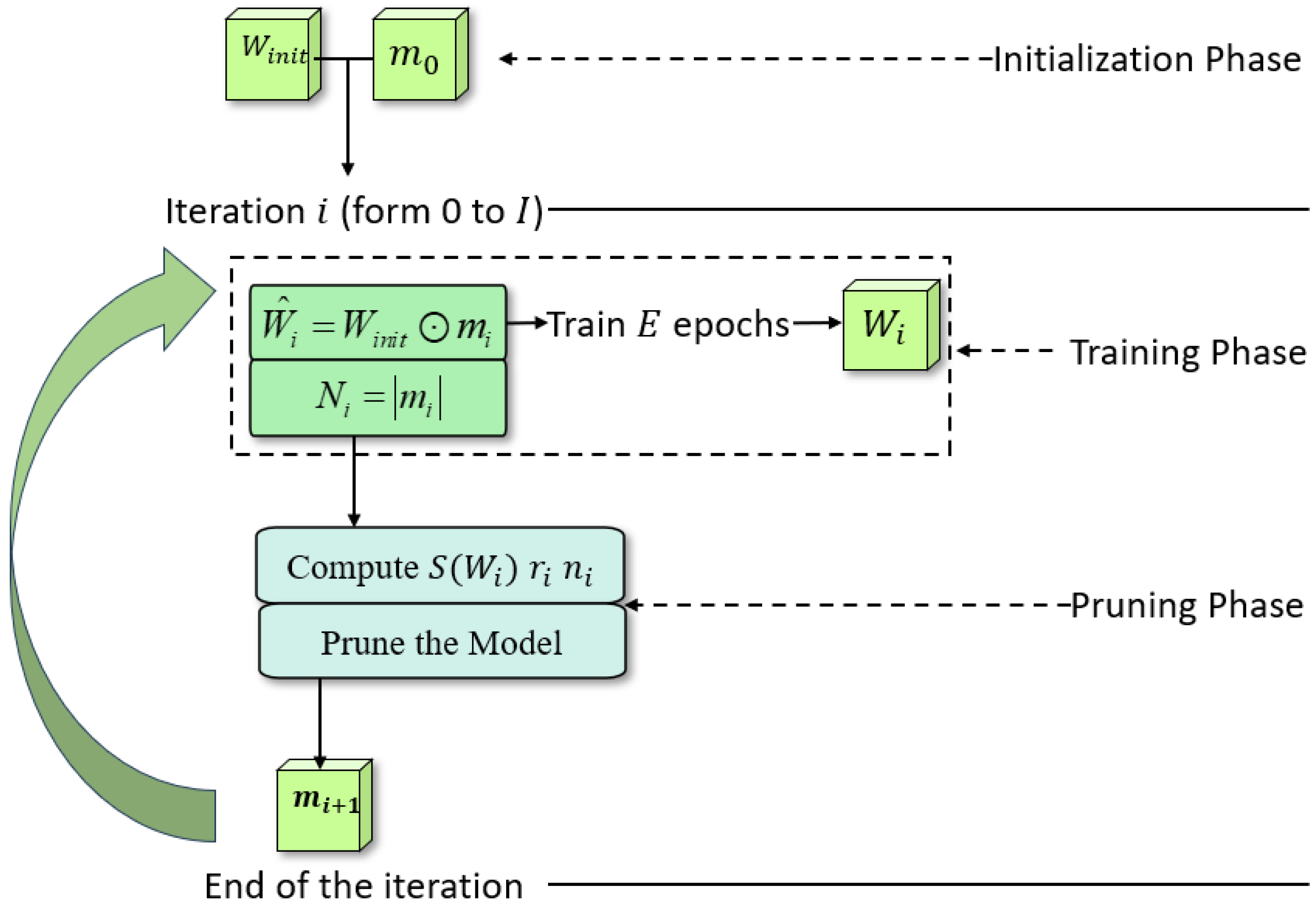
2.3.2. Dynamic Pruning Algorithm Based on Sparsity

Frankle and Cabin proposed the famous lottery ticket pruning algorithm [46]. They argue that when a model possesses a certain degree of sparsity, over-parameterized networks can be effectively pruned, reinitialized, and retrained. They also propose that training from a randomly initialized set of parameters yields a network with superior performance compared to training from scratch. The dynamic pruning algorithm based on sparsity is inspired by these two points of view proposed by the lottery ticket pruning algorithm. The following is a description of the algorithm flow. Before the pruning starts, the parameters of the network model are randomly initialized, and at each iteration, we start training the network from the initialized parameters. We represent it using $W_{init}$. At the same time, before the iteration starts, a pruning mask $m_0$ is initialized with all ones, which means that on the first iteration, we will keep all the parameters for the full training of the model. The advantage of using the mask to perform multiple iterations of pruning is that it will not cause too much damage to the performance of the network, pruned parameters may be freed in subsequent iterations until the end of the final iteration to produce the most suitable mask. For each iteration $i=0,1,2,3,...I$, we can get model parameters ${\tilde{W}}_i$ and the number of parameters $N_i$, they can be computed as follows:

$${\tilde{W}}_i=W_{init}\odot m_i,N_i=\left|m_i\right|$$

(11)

in each iteration, we use $m_i$ to freeze the gradient and train the model from ${\tilde{W}}_i$, after training for E epochs we obtain the model parameters $W_i$. Now it’s the time to prune the model, but a fixed pruning rate may result in under-pruned or over-pruned, an under-pruned model requires more iterations and more computing resources to obtain a better small neural network, while an over-pruned model cannot maintain the expected performance. So we computed $S\left(W_i\right)$ then calculate the lower bound $r_i$ of the parameter size of the pruned model according to Formula (10):

$$r_i=d{(1+k)}^{\frac{-q}{q-p}}{[1-S(T\left)\right]}^{\frac{qp}{q-p}},$$

(12)

then we compute the number of pruned model parameters $n_i$:

$$n_i=N_i·min(1-\frac{r_i}{N_i},\alpha )$$

(13)

where $\alpha$ is the maximum pruning ratio, we set $\alpha =0.9$ to prevent over-pruned. Finally, we use these computations to prune the model and create a new mask $m_{i+1}$ for the next pruning iteration. Model parameters $W_i$ and mask $m_i$ are saved in each iteration. Figure 4 is the schematic diagram of the complete flow of the algorithm.

3. Collection and Preprocessing of Dataset

The collection of EAB larvae’s boring vibration signals started on 23 July 2021 and ended on 27 July 2021. Firstly, under the guidance of professional foresters, we selected several trees infested with EAB larvae from a forest farm in Tongzhou, Beijing, and then cut the trunks into equal-length segments. To ensure data diversity we selected trees in different conditions, including living, dying, and dead. Finally we got 6 trunk segments from living trees, 4 trunk segments from dying trees, and 2 from dead trees. We use self-developed vibration signal acquisition equipment for data collection, which was jointly developed by Beijing Forestry University and Beihang University. The specific method of operation is to insert the equipment’s probe into the tree trunk to record the vibration signals produced by EAB larvae. For each trunk segment, before the collection started, we monitored the larvae activity using headphones to confirm it was active. The entire data collection process took place in a quiet experimental environment to ensure the purity of the original vibration signals.

The collection of SCM larvae’s boring vibration signals started on 29 July 2023 and ended on 14 August 2023. We selected several trees infested with SCM larvae from a forest farm in Wangzhuang Village, Shunyi, Beijing, and we got 2 trunk segments from living trees, 2 from dying trees, and 1 from dead trees. We used the same equipment and methods similar to the collection process of EAB dataset. The difference is that when collecting SCM data, the probe is inserted deeper, because SCM larvae mainly feed on the xylem of trees.

To ensure the accuracy of the data, we took several measures throughout the data collection process:

• We carefully calibrated and tested our vibration signal collector to ensure its reliability and accuracy in capturing the signals. We also followed strict protocols during the data collection, ensuring consistent placement of the probes and maintaining stable recording conditions.
• We cross-validated the collected data by conducting multiple rounds of data collection for each tree segment. This helped to minimize any potential variability or outliers in the dataset.
• The visual inspection of the larvae inside the tree trunks served as an additional validation step, which means after data collection, we peeled off the bark under the guidance of the forestry personnel and directly observed EAB larvae and SCM larvae inside the trunk.

Overall, by implementing rigorous procedures, we took the necessary steps to ensure the accuracy and reliability of the dataset. The data of EAB and SCM are independent of each other and form their own data sets. Figure 5 shows some photos taken during the dataset collection process.

After obtaining the raw dataset, we performed basic preprocessing using manual methods. Due to the need for staff to start and shut down the equipment during the collection process, some environmental noise will inevitably occur, especially at the beginning and end of the audio. And the larvae won’t always eat the tree, so there will be some noticeable blank periods. These audio segments and other obviously noisy segments will be removed during dataset preprocessing.

In addition, we collected a series of different environmental noises to generate noisy vibration signals. This is a commonly used method in the field of speech enhancement, which combines ambient noise with clean voice, and the datasets of EAB and SCM use the same environmental noise. This approach creates a dataset that mimics real-world scenarios. In order to do this, we chose some places similar to the forest environment, four of the selected locations are at Beijing Forestry University and one is at the Beijing Olympic Park. We use the same equipment and measures as for collecting vibration signals. We preprocess these noise signals similarly to pure vibration signals, discarding blank segments that do not contain noise, which can ensure efficient model training.

After completing the preprocessing, we divide the vibration signal and environmental noise into small segments of 3 s. In order to generate the vibration signal with noise in the training set, we divide 90 percent of the pure vibration signal segments and environmental noise segments according to different signal-to-noise ratio is mixed, and the remaining 10 percent of the vibration signal and environmental noise are also mixed according to same SNR as a test set. And during the training process, we use 5 percent of the training set data for verification. The total duration of the EAB training set is about 22 h, and the total duration of the EAB test set is about 2.5 h. As for the SCM dataset, they are 27 h and 3 h respectively.

4. Experiment

4.1. Experimental Setup

For vibration signal enhancement model, we choose Hanning window in the STFT, and the window length is 25 ms, which leads to the dimension of the frequency feature of the input network being 601, so the size of the model input is (1, 601, 161, 2). Regarding the pruning algorithm, we set up four different experiments to verify the feasibility and effectiveness of combining the pruning algorithm and lightweight vibration signal enhancement model. We use three pruning algorithms, the first is the one-shot (OS) pruning, the specific content is after the model training is completed, the model will be pruned according to the importance of neurons and then fine-tuned to obtain the final compressed model. The second is the lottery ticket pruning algorithm (LTP), and the third is the dynamic pruning algorithm based on sparsity (DPAS) introduced above. Among them, the lottery ticket pruning algorithm is used as the baseline in terms of the pruning effect. We set a fixed pruning ratio of 0.1 in LTP. We set $p=0.5$ and $q=1$ in DPAS, and we chose $k=0$. We do 15 iterations of pruning on both LTP and DPAS. The processor of the hardware used to train the model in our experiments is 11th Gen Intel Core i7-11700 with 16 GB memory, and the graphics card is NVIDIA TITAN RTX. In addition, we use another platform to test the model’s performance. The processor of this platform is AMD Ryzen 5 5600U with Radeon Graphics with 16 GB memory.

4.2. Evaluation Metrics

Our model is used to enhance vibration signals and does not involve human auditory perception, therefore, evaluation indicators such as perceptual evaluation of speech quality (PESQ) are not suitable for this model. We use signal-to-noise ratio (SNR) and log-likelihood ratio (LLR) when evaluating model performance. SNR is an indicator used to measure the relative strength between signal and noise. A higher SNR means that the signal has higher clarity and higher quality. The LLR represents the ratio of the energies of the prediction residuals of the enhanced and clean signals, a higher LLR generally indicates a clearer signal For assessing the effect of the pruning algorithm, we mainly compare the parameters of the model after pruning and the inference time on the CPU. The number of parameters can intuitively reflect the model’s size, and small models are easier to deploy on embedded edge devices in the forest. The inference time can reflect the performance and efficiency of the model, a model with a shorter inference time consumes fewer computing resources and is conducive to the real-time enhancement of the vibration signal to detect the pests more quickly. The computational methods of SNR and LLR are shown as following formulas:

$$SNR=10{log}_{10}\frac{{\sum }_{n=0}^{N-1}{v}^2\left(n\right)}{{\sum }_{n=0}^{N-1}(v^2\left(n\right)-{\widehat{v}}^2\left(n\right))}$$

(14)

$$LLR({\mathrm{s}}_x,s_{\widehat{x}})=log\frac{{\overline{s}}_{\widehat{x}}^T{R}_x{\overline{s}}_{\widehat{x}}}{s_x^T{R}_x{s}_x}$$

(15)

In the formula of SNR, v represents the clean vibration signal, and $\widehat{v}$ is the enhanced vibration signal. N is the number of samples. In the formula of LLR, $s_x^T$ is the LPC (Linear Predictive Coding) coefficients of the clean signal, ${\overline{s}}_{\widehat{x}}^T$ is the LPC coefficients of the enhanced signal, and $R_x$ is the auto-correlation matrix of the clean signal. We use some library functions in Python to obtain the number of parameters and record them in each pruning method and each iteration. The timestamp is used to calculate the inference time of the model when the inference program is executed.

4.3. Details of Experiments

4.3.1. Experiment I

In the experiment I, we fully trained the lightweight vibration signal enhancement model using the EAB dataset and the SCM dataset respectively. We tested the performance of the model under different SNR conditions according to the above evaluation metrics. We use this model as a baseline and original model in terms of model performance.

4.3.2. Experiment II

In the experiment II, we use DPAS, LTP, and One-Shot to compress our models respectively and compare the results of different pruning algorithms. The lottery ticket pruning function will judge whether to continue pruning at the end of each iteration, to make it possible to complete 15 iterations, we expand the constraint range of performance degradation a little. Otherwise, it will end the iteration early. Then we will compare the compressed model with the original model.

4.3.3. Experiment III

To futher demonstarte the advantages of our method, we compare this method with the results of similar previous studies, including Dual-Vibration Enhancement Network (DVEN) [47], VibDenoiser [48], and the Time-domain Conformer-based Enhancement Network for Vibration (T-CENV) [49]. We use the EAB dataset to compare our method with these three models according to three metrics, including parameters of model, infertime and enhancement performance.

4.3.4. Experiment IV

In this experiment, we compare the detection accuracy of noisy vibration signals and vibration signals enhanced by our model on two well-known classification models: EcapaTDNN [50] and ResNetSE. We use the same dataset source as the vibration signal enhancement model to train the classification model, which contains 2995 signals from infested trees and 1426 from uninfested trees. The classification labels are infested and uninfested. We use the non-enhanced noise vibration signal and the enhanced vibration signal for classification under different signal-to-noise ratios.

5. Results

5.1. Results and Analysis of Experiment I

Table 1. The enhancement performance of lightweight vibration enhancement model using EAB dataset under different SNR conditions.

Metrics	0 dB	−2.5 dB	−5 dB	−7.5 dB	−10 dB	Average
SNR	16.8637	15.1525	13.5645	11.7643	10.3246	13.5339
LLR	0.0658	0.0762	0.1467	0.2485	0.3478	0.1769
InferTime (s) 1	144.89	148.05	144.26	144.26	146.58	145.61

¹ The total duration of the noisy vibration signal used for testing is 1800s. The data in the table shows the time it takes for all these vibration signals to be enhanced by the model.

shows the specific test results of EAB dataset, and

Table 2. The enhancement performance of lightweight vibration enhancement model using SCM dataset under different SNR conditions.

Metrics	0 dB	−2.5 dB	−5 dB	−7.5 dB	−10 dB	Average
SNR	17.0834	15.4113	13.5786	12.1928	10.3559	13.7244
LLR	0.0681	0.0787	0.1476	0.2550	0.3446	0.1788
InferTime (s)	141.39	149.28	148.44	139.60	147.57	145.25

shows the results of SCM dataset.

From Table 1 and Table 2, we can see that the performance of the models using the EAB dataset and the SCM dataset is almost same. We believe this is because the boring vibration signals of different trunk borers are similar, which also illustrates the general applicability of our method to the detection of different trunk borers. In the subsequent discussion of results, we mainly focus on the model trained using the EAB dataset. The number of model parameters without pruning is only 0.88 M. We have achieved a good enhancement effect on vibration signals with very few parameters.

5.2. Results and Analysis of Experiment II

Form the Figure 6, it can be clearly seen that the DPAS pruning is slow but highly precise, with almost no decrease in model performance. The LTP shows a clear performance degradation from the 9th iteration onwards. If the constraint on the allowed decrease in performance is narrowed down, the LTP will terminate prematurely. The one-shot pruning reduces the model’s parameters by 40.9%, but further compressing will be very difficult because it cannot precisely assess the importance of neurons, further compressing may lead to performance collapse. The results indicate that the LTP is suitable for networks with higher redundancy, and DPAS is suitable for achieving further and more refined mode compression. The results also show that our lightweight vibration signal enhancement model has reached a relatively compact level before it is compressed. The variation curve of the sparsity in Figure 7 also proves this point.

We selected the model after 15 iterations of DPAS and the model pruned after 8 iterations of LTP, and compared them with the original model.

Table 3. Comparison of the model pruned by DPAS and LTP respectively with the original model.

	Parameters	InferTime (s)	Average SNR (dB)	Average LLR
Original	884,928	145.61	13.5339	0.1769
DPAS	337,038	113.35	13.1144	0.2899
percentage change 1	−62%	−22%	−3%	+63%
LTP	423,257	119.77	12.1589	0.2978
percentage change	−52%	−17%	−10%	+68%

¹ Percentage change indicates the change in each evaluation metrics of the model pruned by two pruning algorithms (DPAS and LTP) compare with the original network.

is the detailed data.

From Table 3, we can draw a very obvious conclusion: the model pruned by the DPAS is better, in the case of pruning 62% of the parameters, 22% reduction in inference time, the SNR only dropped by 3%. So the lightweight vibration enhancement model that compressed by DPAS is our final best choice, we named it as VibEnh-DPAS. Figure 8 shows the spectrogram and waveform diagram of the vibration signal before and after enhancement.

5.3. Results and Analysis of Experiment III

From

Table 4. Comparison of VibEnh-DPAS with DVEN, VibDenoiser and T-CENV.

Model	Param. (M)	%${\mathit{\Delta }}_1$	InferTime (s)	%${\mathit{\Delta }}_2$	SNR (dB)	%${\mathit{\Delta }}_3$
DVEN	1.32	−74.2%	165.6	−31.5%	18.73	−12.3%
VibDenoiser	10.75	−96.8%	273.6	−58.5%	18.57	−11.6%
T-CENV	4.23	−91.9%	195.8	−42.1%	17.84	−7.96%
VibEnh-DPAS	0.34	-	113.4	-	16.42	-

%${\Delta }_1$ is the percentage change of the parameters of VibEnh-DPAS compared to DVEN, VibDenoiser, and T-CENV respectively. %${\Delta }_2$ and %${\Delta }_3$ are the percentage changes of inference time and SNR respectively.

, we can intuitively see that in terms of the number of parameters, our method reduced by 74.2%, 96.8% and 91.9% respectively compared with these three models. Regarding inference time, they are reduced by 31.5%, 58.5% and 42.1% respectively. And the enhancement performance only reduced a little bit, which has almost no impact on subsequent pest detection accuracy. These data demonstrate that our method is highly beneficial for model deployment in natural forest environments.

5.4. Results and Analysis of Experiment IV

Figure 9 shows the accuracy of classification based on different data.

It is obvious that the higher the signal-to-noise ratio, the higher the classification accuracy. The accuracy of classification using the enhanced vibration signal is significantly improved. And similar to the previous comparison results, the model pruned by DPAS shows minimal reduction in performance when compared to the original model.

6. Discussion

Accurate and timely detection of trunk borers remains a challenging task. A effective method is to detect trunk borer larvae through the wood-boring vibration signal produced by the larvae feeding in the trunk. As state in a previous study, environment noise can be significant and cover the feeble vibrations of wood-boring insects [51], thus having a negative impact on the detection accuracy. And it is difficult to deploy technology with high hardware resource requirements in the wild environment. Previous studies have proven that machine learning-based techniques can be applied to the processing of boring vibration signals [52]. We propose a lightweight vibration signal enhancement model and use a dynamic pruning algorithm based on sparsity to compress it to achieve the goal of being small and compact. We combine the features of convolutional recurrent neural network and Transformer, use multi-head mechanism instead of RNN for intra-block processing, and retain inter-block RNN. To conduct our research, We use self-developed equipment to collect vibration signals of EAB and SCM larvae while they are feeding in the trees.

To prove the effectiveness and reliability of our method, we conducted some experiments and analyzed the experimental results. Through the comparison of models using different data sets in Experiment I, we conclude that our model achieves good signal enhancement effects and has good generalization. In Experiment II, we compared different pruning algorithms and proved that the DPAS we proposed is more effective. We name the model compressed using the pruning algorithm VibEnh-DPAS. Our method is characterized by being lightweight and having a small number of parameters, Experiment III proves this point. Compared with the three methods DVEN, VibDenoiser, and T-CENV, our method achieves almost the same performance using fewer parameters and faster inference speed. We tested the effect of the vibration signal enhanced by our method on the detection accuracy in Experiment IV, results show that our method has significantly improved the detection accuracy. All these experimental results prove that our method to the problem of difficulty in early detection of trunk borers is effective and practical.

Our work provides an idea for future real-time detection of trunk borer larvae. For example, deploying our model onto an enbeded FPGA board (Field Programmable Gate Array), which is cost-effective, fast in computation, and low in power consumption, but has limited storage and computational resources [53], and we will also further develop optimization solutions tailored for FPGA platforms in future. The biggest limitation of our study is that we only have two datasets. So, the first step in subsequent research is to enrich our dataset. In this paper, the dataset we used only consists of vibration signals produced by EAB larvae and SCM larvae feeding in trees because there are scarce datasets available in the field of pest control that are similar to the one used in this study. Therefore, expanding our dataset to train a universally applicable model is the top priority. On the other hand, optimizing the model is also very important. Future models should aim at fewer parameters, faster inference, and less computing resource consumption, which is of great significance to the deployment of the model, and will promote the establishment of an all-round early warning system to protect forest areas everywhere. It is worth mentioning that this technology can also be used for other types of vibration signal enhancement, such as pest detection in buildings [54], moth detection inside wooden furniture, etc. With the continuous development of technology and the improvement of hardware performance, we believe that our method will be further applied to solve more problems.

References

1. Jha, K.; Doshi, A.; Patel, P.; Shah, M. A comprehensive review on automation in agriculture using artificial intelligence. Intell. Agric. 2019, 2, 1–12. [Google Scholar] [CrossRef]
2. Pearce, D.W.; Pearce, C.G. The Value of Forest Ecosystems; Centre for Social and Economic Research on the Global Environment (CSERGE): Norfolk, UK, 2001. [Google Scholar]
3. Fiala, P.; Friedl, M.; Cap, M.; Konas, P.; Smira, P.; Naswettrova, A. Non destructive method for detection wood-destroying insects. In Proceedings of the PIERS Proceedings, Guangzhou, China, 25–28 August 2014; pp. 1642–1646. [Google Scholar]
4. Sutin, A.; Yakubovskiy, A.; Salloum, H.R.; Flynn, T.J.; Sedunov, N.; Nadel, H. Towards an automated acoustic detection algorithm for wood-boring beetle larvae (Coleoptera: Cerambycidae and Buprestidae). J. Econ. Entomol. 2019, 112, 1327–1336. [Google Scholar] [CrossRef] [PubMed]
5. Farr, I.; Chesmore, D. Automated Bioacoustic Detection and Identification of Wood-Boring Insects for Quarantine Screening and Insect Ecology; University of York: York, UK, 2007; pp. 201–208. [Google Scholar]
6. Mankin, R.W.; Mizrach, A.; Hetzroni, A.; Levsky, S.; Nakache, Y.; Soroker, V. Temporal and spectral features of sounds of wood-boring beetle larvae: Identifiable patterns of activity enable improved discrimination from background noise. Fla. Entomol. 2008, 91, 241–248. [Google Scholar] [CrossRef]
7. Bilski, P.; Bobiński, P.; Krajewski, A.; Witomski, P. Detection of wood boring insects’ larvae based on the acoustic signal analysis and the artificial intelligence algorithm. Arch. Acoust. 2016, 42, 61–70. [Google Scholar] [CrossRef]
8. Korinšek, G.; Tuma, T.; Virant-Doberlet, M. Automated vibrational signal recognition and playback. In Biotremology: Studying Vibrational Behavior; Springer: Berlin/Heidelberg, Germany, 2019; pp. 149–173. [Google Scholar]
9. Sun, Y.; Tuo, X.; Jiang, Q.; Zhang, H.; Chen, Z.; Zong, S.; Luo, Y. Drilling vibration identification technique of two pest based on lightweight neural networks. Sci. Silvae Sin. 2020, 56, 100–108. [Google Scholar]
10. Wang, D.L. On ideal binary mask as the computational goal of auditory scene analysis. In Speech Separation by Humans and Machines; Springer: Berlin/Heidelberg, Germany, 2005; pp. 181–197. [Google Scholar]
11. Wang, D.; Brown, G.J. Computational Auditory Scene Analysis: Principles, Algorithms, and Applications; Wiley: Hoboken, NJ, USA; IEEE: Piscataway, NJ, USA, 2006. [Google Scholar]
12. Wang, D.; Chen, J. Supervised speech separation based on deep learning: An overview. IEEE/ACM Trans. Audio Speech Lang. Process. 2018, 26, 1702–1726. [Google Scholar] [CrossRef] [PubMed]
13. Wang, Y.; Wang, D. Towards scaling up classification-based speech separation. IEEE Trans. Audio Speech Lang. Process. 2013, 21, 1381–1390. [Google Scholar] [CrossRef]
14. Healy, E.W.; Yoho, S.E.; Wang, Y.; Wang, D. An algorithm to improve speech recognition in noise for hearing-impaired listeners. J. Acoust. Soc. Am. 2013, 134, 3029–3038. [Google Scholar] [CrossRef]
15. Weninger, F.; Hershey, J.R.; Le Roux, J.; Schuller, B. Discriminatively trained recurrent neural networks for single-channel speech separation. In Proceedings of the 2014 IEEE Global Conference on Signal and Information Processing (GlobalSIP), Atlanta, GA, USA, 3–5 December 2014; pp. 577–581. [Google Scholar]
16. Weninger, F.; Erdogan, H.; Watanabe, S.; Vincent, E.; Le Roux, J.; Hershey, J.R.; Schuller, B. Speech enhancement with LSTM recurrent neural networks and its application to noise-robust ASR. In Proceedings of the Latent Variable Analysis and Signal Separation: 12th International Conference, LVA/ICA 2015, Liberec, Czech Republic, 25–28 August 2015; pp. 91–99. [Google Scholar]
17. Park, S.R.; Lee, J. A fully convolutional neural network for speech enhancement. arXiv 2016, arXiv:1609.07132. [Google Scholar]
18. Rethage, D.; Pons, J.; Serra, X. A wavenet for speech denoising. In Proceedings of the 2018 IEEE International Conference on Acoustics, Speech and Signal Processing (ICASSP), Calgary, AB, Canada, 15–20 April 2018; pp. 5069–5073. [Google Scholar]
19. Vaswani, A.; Shazeer, N.; Parmar, N.; Uszkoreit, J.; Jones, L.; Gomez, A.N.; Kaiser, Ł.; Polosukhin, I.; Polosukhin, I. Attention is all you need. In Proceedings of the Advances in Neural Information Processing Systems, Long Beach, CA, USA, 4–9 December 2017; Volume 30. [Google Scholar]
20. Chen, J.; Lu, Y.; Yu, Q.; Luo, X.; Adeli, E.; Wang, Y.; Lu, L.; Yuille, A.L.; Zhou, Y. Transunet: Transformers make strong encoders for medical image segmentation. arXiv 2021, arXiv:2102.04306. [Google Scholar]
21. Dai, Z.; Yang, Z.; Yang, Y.; Carbonell, J.; Le, Q.V.; Salakhutdinov, R. Transformer-xl: Attentive language models beyond a fixed-length context. arXiv 2019, arXiv:1901.02860. [Google Scholar]
22. Zhou, S.; Dong, L.; Xu, S.; Xu, B. A comparison of modeling units in sequence-to-sequence speech recognition with the transformer on Mandarin Chinese. In Proceedings of the 25th International Conference, ICONIP 2018, Siem Reap, Cambodia, 13–16 December 2018; pp. 210–220. [Google Scholar]
23. Lin, T.; Wang, Y.; Liu, X.; Qiu, X. T-gsa: Transformer with gaussian-weighted self-attention for speech enhancement. In Proceedings of the ICASSP 2020–2020 IEEE International Conference on Acoustics, Speech and Signal Processing (ICASSP), Barcelona, Spain, 9 April 2020; pp. 6649–6653. [Google Scholar]
24. Yu, W.; Zhou, J.; Wang, H.; Tao, L. SETransformer: Speech enhancement transformer. In Cognitive Computation; Springer: Berlin/Heidelberg, Germany, 2022; pp. 1–7. [Google Scholar]
25. Wang, K.; He, B.; Zhu, W.P. TSTNN: Two-stage transformer based neural network for speech enhancement in the time domain. In Proceedings of the ICASSP 2021–2021 IEEE International Conference on Acoustics, Speech and Signal Processing (ICASSP), Toronto, ON, Canada, 13 May 2021; pp. 6649–6653. [Google Scholar]
26. LeCun, Y.; Bottou, L.; Bengio, Y.; Haffner, P. Gradient-based learning applied to document recognition. Proc. IEEE 1998, 86, 2278–2324. [Google Scholar] [CrossRef]
27. Brown, T.; Mann, B.; Ryder, N.; Subbiah, M.; Kaplan, J.D.; Dhariwal, P.; Neelakantan, A.; Shyam, P.; Sastry, G.; Askell, A.; et al. Language models are few-shot learners. Adv. Neural Inf. Process. Syst. 2020, 33, 1877–1901. [Google Scholar]
28. Qiu, Z.; Yao, T.; Mei, T. Deep quantization: Encoding convolutional activations with deep generative model. In Proceedings of the IEEE Conference on Computer Vision and Pattern Recognition, Honolulu, HI, USA, 21–26 July 2017; pp. 6759–6768. [Google Scholar]
29. Gong, Y.; Liu, L.; Yang, M.; Bourdev, L. Compressing deep convolutional networks using vector quantization. arXiv 2014, arXiv:1412.6115. [Google Scholar]
30. Young, S.I.; Zhe, W.; Taubman, D.; Girod, B. Transform quantization for CNN compression. IEEE Trans. Pattern Anal. Mach. Intell. 2021, 44, 5700–5714. [Google Scholar] [CrossRef] [PubMed]
31. Haeffele, B.; Young, E.; Vidal, R. Structured low-rank matrix factorization: Optimality, algorithm, and applications to image processing. In Proceedings of the International Conference on Machine Learning, Beijing, China, 22–24 June 2014; pp. 2007–2015. [Google Scholar]
32. Hinton, G.; Vinyals, O.; Dean, J. Distilling the knowledge in a neural network. arXiv 2015, arXiv:1503.02531. [Google Scholar]
33. He, Y.; Zhang, X.; Sun, J. Channel pruning for accelerating very deep neural networks. In Proceedings of the IEEE International Conference on Computer Vision, Venice, Italy, 22–29 October 2017; pp. 1389–1397. [Google Scholar]
34. Pasandi, M.M.; Hajabdollahi, M.; Karimi, N.; Samavi, S. Modeling of pruning techniques for deep neural networks simplification. arXiv 2020, arXiv:2001.04062. [Google Scholar]
35. Wei, X.; Wu, Y.; Reardon, R.; Sun, T.-H.; Lu, M.; Sun, J.-H. Biology and damage traits of emerald ash borer (Agrilus planipennis Fairmaire) in China. Insect Sci. 2007, 14, 367–373. [Google Scholar] [CrossRef]
36. Zhang, L.; Feng, Y.-Q.; Ren, L.-L.; Luo, Y.-Q.; Wang, F.; Zong, S.-X. Sensilla on antenna, ovipositor and leg of E riborus applicitus (Hymenoptera: Ichneumonidae), a parasitoid wasp of H olcocerus insularis staudinger (Lepidoptera: Cossidae). Acta Zool. 2015, 96, 253–263. [Google Scholar] [CrossRef]
37. Krawczyk, M.; Gerkmann, T. STFT phase reconstruction in voiced speech for an improved single-channel speech enhancement. IEEE/ACM Trans. Audio Speech Lang. Process. 2014, 22, 1931–1940. [Google Scholar] [CrossRef]
38. Luo, Y.; Chen, Z.; Yoshioka, T. Dual-path rnn: Efficient long sequence modeling for time-domain single-channel speech separation. In Proceedings of the ICASSP 2020—2020 IEEE International Conference on Acoustics, Speech and Signal Processing (ICASSP), Barcelona, Spain, 4–8 May 2020; pp. 46–50. [Google Scholar]
39. Gehring, J.; Auli, M.; Grangier, D.; Yarats, D.; Dauphin, Y.N. Convolutional sequence to sequence learning. In Proceedings of the 34th International Conference on Machine Learning, Sydney, NSW, Australia, 6–11 August 2017; pp. 1243–1252. [Google Scholar]
40. Liu, X.; Yu, H.-F.; Dhillon, I.; Hsieh, C.-J. Learning to encode position for transformer with continuous dynamical model. In Proceedings of the 37th International Conference on Machine Learning, Virtual Event, 13–18 July 2020; pp. 6327–6335. [Google Scholar]
41. Wang, B.; Zhao, D.; Lioma, C.; Li, Q.; Zhang, P.; Simonsen, J.G. Encoding word order in complex embeddings. arXiv 2019, arXiv:1912.12333. [Google Scholar]
42. Luo, Y.; Mesgarani, N. Conv-tasnet: Surpassing ideal time–frequency magnitude masking for speech separation. IEEE/ACM Trans. Audio Speech Lang. Process. 2019, 27, 1256–1266. [Google Scholar] [CrossRef] [PubMed]
43. Ding, J.; Tarokh, V.; Yang, Y. Model selection techniques: An overview. IEEE Signal Process. Mag. 2018, 35, 16–34. [Google Scholar] [CrossRef]
44. Zhou, Z.; Yu, J. A new nonconvex sparse recovery method for compressive sensing. Front. Appl. Math. Stat. 2019, 5, 14. [Google Scholar] [CrossRef]
45. Wang, W.; Lu, Y. Analysis of the mean absolute error (MAE) and the root mean square error (RMSE) in assessing rounding model. In Proceedings of the IOP Conference Series: Materials Science and Engineering, Kuala Lumpur, Malaysia, 15–16 December 2017; p. 012049. [Google Scholar]
46. Frankle, J.; Carbin, M. The lottery ticket hypothesis: Finding sparse, trainable neural networks. arXiv 2018, arXiv:1803.03635. [Google Scholar]
47. Shi, H.; Chen, Z.; Zhang, H.; Li, J.; Liu, X.; Ren, L.; Luo, Y. Enhancement of Boring Vibrations Based on Cascaded Dual-Domain Features Extraction for Insect Pest Agrilus planipennis Monitoring. Forests 2023, 14, 902. [Google Scholar] [CrossRef]
48. Shi, H.; Chen, Z.; Zhang, H.; Li, J.; Liu, X.; Ren, L.; Luo, Y. A Waveform Mapping-Based Approach for Enhancement of Trunk Borers’ Vibration Signals Using Deep Learning Model. Insects 2022, 13, 596. [Google Scholar] [CrossRef] [PubMed]
49. Zhang, H.; Li, J.; Cai, G.; Chen, Z.; Zhang, H. A CNN-Based Method for Enhancing Boring Vibration with Time-Domain Convolution-Augmented Transformer. Insects 2023, 14, 631. [Google Scholar] [CrossRef]
50. Desplanques, B.; Thienpondt, J.; Demuynck, K. Ecapa-tdnn: Emphasized channel attention, propagation and aggregation in tdnn based speaker verification. arXiv 2020, arXiv:2005.07143. [Google Scholar]
51. Potamitis, I.; Rigakis, I.; Tatlas, N.-A.; Potirakis, S. In-vivo vibroacoustic surveillance of trees in the context of the IoT. Sensors 2019, 10, 1366. [Google Scholar] [CrossRef]
52. Liu, X.; Zhang, H.; Jiang, Q.; Ren, L.; Chen, Z.; Luo, Y.; Li, J. Acoustic Denoising Using Artificial Intelligence for Wood-Boring Pests Semanotus bifasciatus Larvae Early Monitoring. Sensors 2022, 22, 3861. [Google Scholar] [CrossRef]
53. Lacey, G.; Taylor, G.W.; Areibi, S. Deep learning on fpgas: Past, present, and future. arXiv 2016, arXiv:1602.04283. [Google Scholar]
54. Querner, P. Insect pests and integrated pest management in museums, libraries and historic buildings. Insects 2015, 6, 595–607. [Google Scholar] [CrossRef] [PubMed]
Figure 1. The overall structure of the model. S is the original vibration signal with noise. S ^ is the signal enhanced by model. Use a skip connection between the corresponding encoder and decoder. The real-part decoder and imaginary-part decoder are used to reconstruct the real and imaginary parts of the spectrum, respectively.
Forests 14 02001 g001
Figure 2. The detailed structure of the processing block. C dimensional local features are extracted by the encoder for every bin in the signal spectrogram. F denotes the frequency dimension compressed by the convolutional encoder. T denotes the time domain.
Forests 14 02001 g002
Figure 3. Schematic diagram of attention mechanism. (a) Self-attention mechanism. (b) The multi-head attention block.
Forests 14 02001 g003
Figure 4. The schematic diagram of the complete flow of the algorithm.
Forests 14 02001 g004
Figure 5. Some photos taken during the dataset collection process. (a) Collection of EAB dataset. (b) After the collection was completed, the bark was peeled off to see the active EAB larvae, which was marked with a red circle in the figure. (c) Collection of SCM dataset. (d) Same as figure (b), we can clearly see the SCM larvae inside the trunk. (e) Insert the probe of the equipment into the tree trunk during data collection in a real forest environment. (f) The researchers monitored the larvae activity using headphones to confirm it was active.
Forests 14 02001 g005
Figure 6. Comparison of three pruning algorithms. (a) Variation curve of the number of parameters for each iteration. (b) Variation curve of the value of loss function for each iteration. One-shot pruning only prunes once, so it is represented as a point in the graph.
Forests 14 02001 g006
Figure 7. The variation curve of the sparsity S ( W ) for each iteration of DPAS.
Forests 14 02001 g007
Figure 8. The spectrogram and waveform diagram of the vibration signal. (ac) are the spectrogram and waveform diagram of the vibration signal before enhancement. (df) are the spectrogram and waveform diagram of the vibration signal after enhancement. Where (a) corresponds to (b,d) corresponds to (c,e) corresponds to (f).
Forests 14 02001 g008
Figure 9. Comparison of classification accuracy on noisy vibration signal, enhanced vibration signal. The signal was enhanced by the original model, the model pruned by DPAS and the model pruned by LTP respectively. (a) Classify using ResNetSE. (b) Classify using EcapaTDNN.
Forests 14 02001 g009