Mapping Mangrove Above-Ground Carbon Using Multi-Source Remote Sensing Data and Machine Learning Approach in Loh Buaya, Komodo National Park, Indonesia

Seftiawan Samsu Rijal; Tien Dat Pham; Salma Noer’Aulia; Muhammad Ikbal Putera; Neil Saintilan

doi:10.3390/f14010094

,

and

¹

Marine Science Study Program, Faculty of Fisheries and Marine Science, Universitas Brawijaya, Malang 65145, Jawa Timur, Indonesia

²

School of Natural Sciences, Faculty of Science and Engineering, Macquarie University, Sydney, NSW 2109, Australia

³

Komodo National Park, Ministry of Environment and Forestry Republic of Indonesia, Labuan Bajo 86554, Nusa Tenggara Timur, Indonesia

^*

Author to whom correspondence should be addressed.

Forests2023, 14(1), 94;https://doi.org/10.3390/f14010094

This article belongs to the Special Issue Biomass Estimation and Carbon Stocks in Forest Ecosystems

Version Notes

Order Reprints

Abstract

Mangrove forests provide numerous valuable ecosystem services and can sequester a large volume of carbon that can help mitigate climate change impacts. Modeling mangrove carbon with robust and valid approaches is crucial to better understanding existing conditions. The study aims to estimate mangrove Above-Ground Carbon (AGC) at Loh Buaya located in the Komodo National Park (Indonesia) using novel Extreme Gradient Boosting (XGB) and Genetic Algorithm (GA) analyses integrating multiple sources of remote sensing (optical, Synthetic Aperture Radar (SAR), and Digital Elevation Model (DEM)) data. Several steps were conducted to assess the model’s accuracy, starting with a field survey of 50 sampling plots, processing the images, selecting the variables, and examining the appropriate machine learning (ML) models. The effectiveness of the proposed XGB-GA was assessed via comparison with other well-known ML techniques, i.e., the Random Forest (RF) and the Support Vector Machine (SVM) models. Our results show that the hybrid XGB-GA model yielded the best results (R² = 0.857 in the training and R² = 0.758 in the testing phase). The proposed hybrid model optimized by the GA consisted of six spectral bands and five vegetation indices generated from Sentinel 2B together with a national DEM that had an RMSE = 15.40 Mg C ha⁻¹ and outperformed other ML models for quantifying mangrove AGC. The XGB-GA model estimated mangrove AGC ranging from 2.52 to 123.89 Mg C ha⁻¹ (with an average of 57.16 Mg C ha⁻¹). Our findings contribute an innovative method, which is fast and reliable using open-source data and software. Multisource remotely sensed data combined with advanced machine learning techniques can potentially be used to estimate AGC in tropical mangrove ecosystems worldwide.

Keywords:

mangroves; Above-Ground Carbon (AGC); remote sensing; Sentinel; machine learning; Indonesia

1. Introduction

Mangroves provide many important ecological and provisioning services including the sequestration of atmospheric CO₂ [1], protection of shorelines from the impact of waves, storm surges, and shoreline erosion [2], and habitat for organisms including shorebirds and commercially important fish [3,4], such that total ecosystem value has been estimated at more than a million dollars per year [5,6]. Despite their valuable contributions, these forests have been lost all over the world due to multiple factors, though primarily human disturbance, especially in Southeast Asia [7]. Previous studies by Fauzi [8] and Latiff [9] revealed that mangrove forests were converted into agriculture, aquaculture, infrastructure, and other land use. Understanding the driving forces and the efficacy of conservation and rehabilitation activities is a central consideration in sustainable mangrove forest replantation and management [10].

One of the fundamental aspects of the sustainable conservation of mangrove forests is to understand their spatial distribution and rates of change, the subject of several previous studies [11,12,13]. However, these forests are associated with a wide range of biophysical parameters that can be related to ecosystem health, interactions, functions, and dynamics [14]. Measuring biophysical parameters of mangroves such as their ability to sequester carbon can be achieved with accuracy using allometric equations applied to field-based measures from designated plots [15]. However, this method is laborious and time-consuming, and often logistically challenging due to the complexity of the mangrove environment, consisting of dynamic tidal levels [16] and tidal cycles [17], and dangerous fauna [18]. Therefore, the development of effective and efficient mangrove carbon estimates is needed.

Remote sensing is an important complementary tool in offering a synoptical overview, high spectral and spatial resolution, and ease of data capture to overcome some of the limitations of time, labor cost, and inaccessibility facing mangrove carbon measurement [19]. The use of remotely sensed optical and Synthetic Aperture Radar (SAR) images incorporated with field-based sampling has been successfully applied to develop mangrove carbon models calibrated by empirical measures [20]. However, a concern for previous studies has been the need for improved accuracy in mangrove carbon models [21]. This issue has driven previous studies to build many models from linear/multi-linear regression from single or combinations of remote sensing image transformations to map mangrove above-ground biomass and above-ground carbon. Furthermore, they may also integrate optical and SAR data to achieve better model prediction [22].

Several optical and SAR remote sensing satellite image libraries are available online and free access, especially for coarse (30 m) and medium-high (20–10 m) spatial resolutions, for instance, generations of Landsat and Sentinel missions [23,24,25]. Landsat yields satisfactory results when used for mangrove extent mapping and temporal changes [26,27]. However, it only works well for large geographical areas and shows inconsistencies in application over finer mapping scales [28]. Sentinel, which brings optical and SAR wavelength with higher spatial resolution, has proven to map mangroves well at large scales [22,28].

The emergence of high-performance computing [29,30], and the use of Machine Learning (ML) techniques can assist in the development of mangrove biomass and carbon maps based on remotely sensed variables [31,32,33,34]. In this study, we aim to test a novel ML method, which was proposed by Pham et al. [35] to map and quantify mangrove above-ground carbon (AGC) in Indonesian mangroves using multisource free-of-charge remotely sensed datasets. Pham et al. [35] developed a novel ML model by integrating the extreme gradient boosting regression (XGB) and genetic algorithm (GA) to map AGB mangroves in Northern Vietnam using optical and SAR data combined with field sampling.

The current work aims to test the effectiveness and robustness of the method using free-of-charge multisource remote sensing data and to extend this approach to other tropical mangrove environments. The results of this study show the ability of the innovative mapping technique using open-source software to perform a mangrove’s carbon while reflecting the optimum features selection to be used.

2. Materials

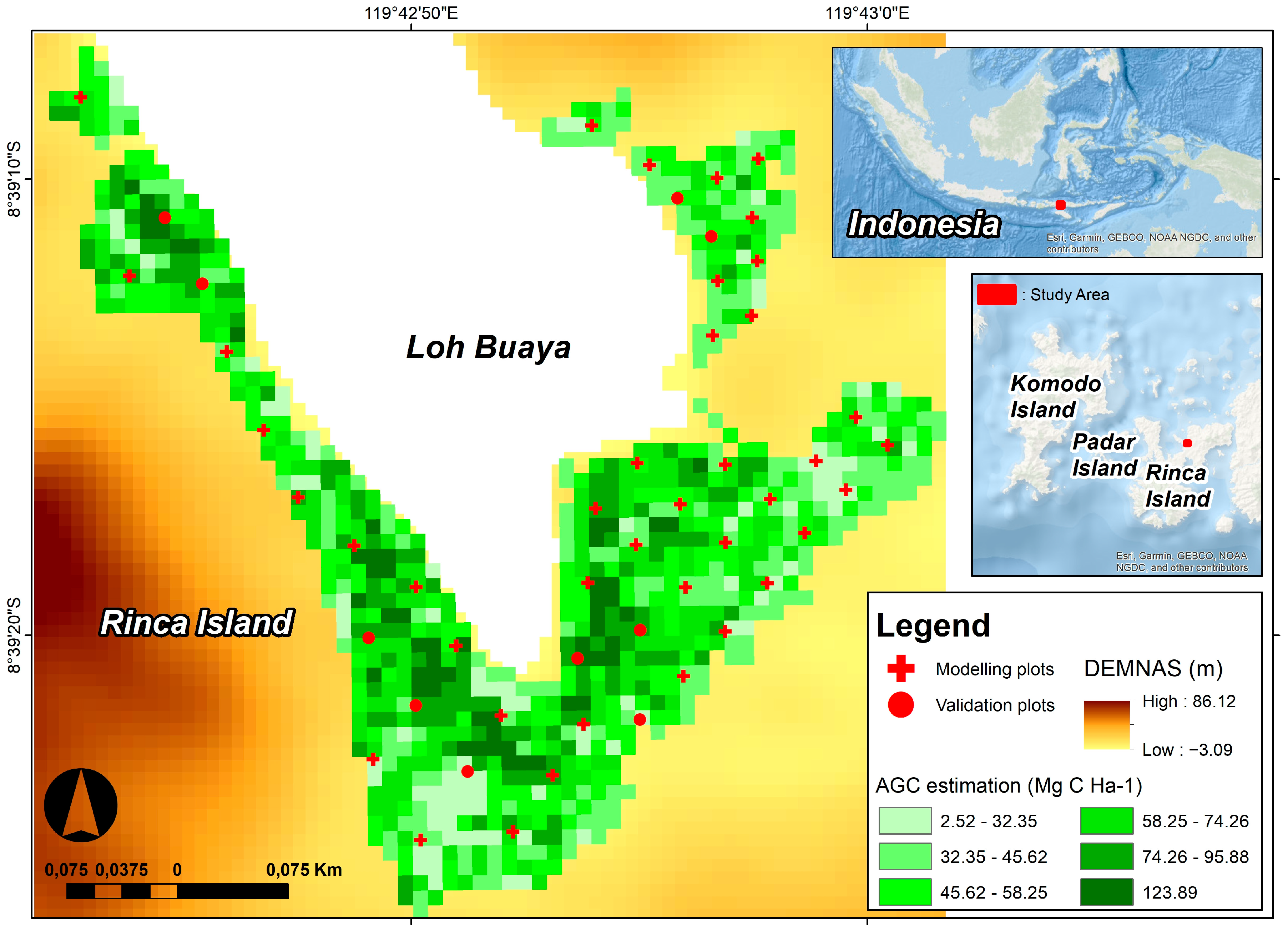
2.1. Study Area

Established on 6th March 1980, Komodo National Park is one of the earliest national parks in Indonesia. The Komodo National Park is an archipelagic national park with a total area of 173,300 ha located at Manggarai Barat Regency, Province of Nusa Tenggara Timur. It has five major islands: Rinca Island, Padar Island, Komodo Island, Gili Motang Island, Nusa Kode Island, and 142 smaller islands [36].

The Komodo National Park has seven different ecosystem types: the quasi-cloud forests (16,706.20 ha), tropical deciduous (monsoon) forests (5026.48 ha), open grassland and woodland savannah (33,788.36 ha), mangroves (1030.30 ha), seagrasses (3967.18 ha), coral reefs (825.61 ha), and the open ocean (111,955.87 ha) [37]. Each ecosystem in the park is unique compared to one another and has a high biodiversity variety, most importantly Loh Buaya Resort.

Loh Buaya is a local name for ‘Crocodile Bay’, which is located on Rinca Island (latitude of 8°32′36″ S; longitude of 119°29′22″ E). Komodo National Park is comprised of 23% terrestrial and 77% aquatic environments. Komodo National Park supports up to 23 species of mangrove [37,38], though to the best of our knowledge no published species list exists.

2.2. Field Survey

Data were collected from 50 plots sampling across four dominant species of mangroves found in the study area: Ceriops decandra, Lumnitzera racemosa, Rhizophora apiculata, and Rhizophora mucronata. Plots consisted of 10 m × 10 m squares established during the field campaign of July 2022 (dry season) using a technique by Dharmawan, 2020 [39] (Figure 1). Measurement in every plot comprised coordinate tagging using a handheld Global Positioning System (GPS: Garmin 64s series with ± 3 m x-y accuracy), Girth at Breast Height (GBH), percentage of canopy cover using hemispherical photography, mangroves species, and substrate identification. MonMang, a smartphone logbook application for mangrove surveys developed by Lembaga Ilmu Pengetahuan Indonesia (LIPI) [40] was used to record field data.

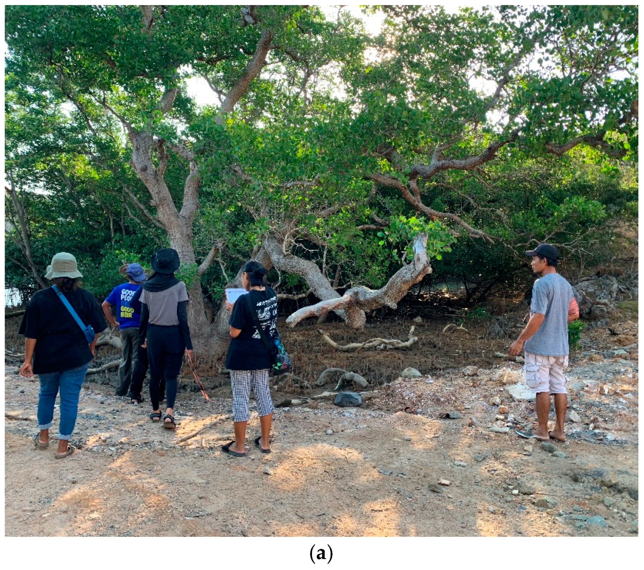
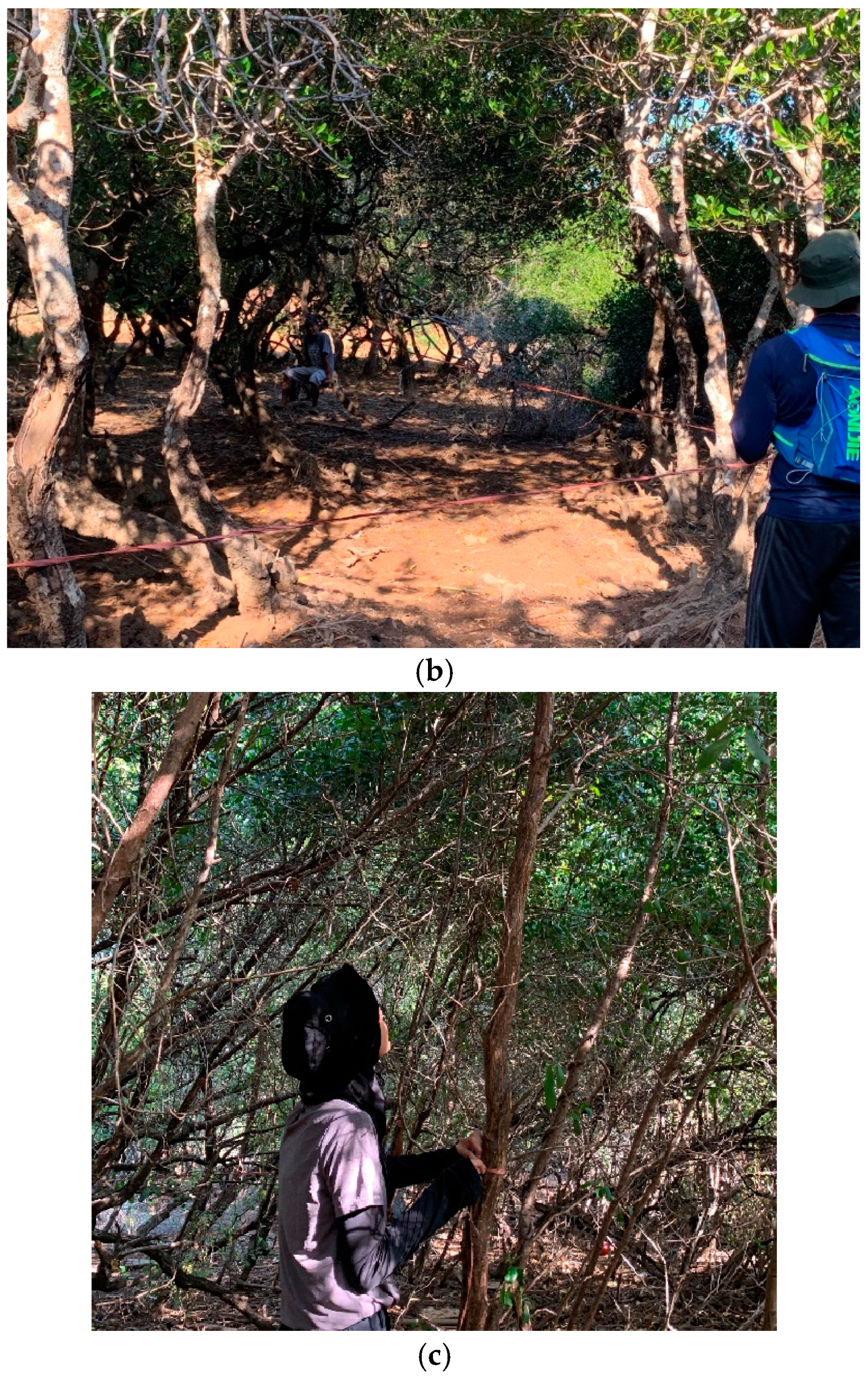
Figure 1. Mangrove field measurement: (a) mangrove situated at the study area, (b) preparing plot measurements using a rope, (c) GBH measurement which is then converted to Diameter of Breast Height (DBH). (Photos taken by Salma Noer ‘Aulia during field survey).

2.3. Biomass and Carbon Estimations

Mangrove GBH was divided by 3.14 to convert into DBH value, and Above-Ground Biomass (AGB) was calculated using the allometric equation (Equation (1)) of Komiyama [41] derived for Southeast Asian mangroves. Therefore, this equation is relevant to use in the study area. The equation is as follows:

AGB (Mg·ha⁻¹) = 0.251ρ(DBH)^2.46

(1)

where:

ρ: Wood density corresponding to the mangrove species, based on the ICRAF database [42]

DBH: Diameter at Breast Height (mean value of different individual trees in every single sampling plot)

According to the Indonesian National Standards for measuring and calculating forest carbon (SNI:7724-2011) [43], about 47% of biomass is carbon. The Above-Ground Carbon (AGC) value was therefore calculated by (Equation (2)).

AGC (Mg C ha⁻¹) = AGB × 0.47

(2)

2.4. Earth Observations (EO) Data

Several earth observation datasets were used in this study including Sentinel-1A (S1A), Sentinel-2B MultiSpectral Instrument (S2B MSI), and Digital Elevation Model Nasional (DEMNAS)/Indonesian Digital Elevation Model to estimate mangrove AGC. S1A is a Synthetic Aperture Radar (SAR) satellite with Level-1 Ground Resolution Distance (GRD) equipped with the frequency of C-band (5.405 GHz) and uses the polarizations of VV (Vertical transmit-Vertical receiving) and VH (Vertical transmit-Horizontal receiving) [44]. S2B MSI level-1C has twelve bands, ranging from 443 nm (coastal band), 492 nm (blue band), 560 nm (green band), 665 nm (red band), 704–783 nm (three red-edge bands), 832 nm (near-infrared (NIR) band), 865 (narrow-NIR band), and 1614–2202 nm (short-wavelength infrared (SWIR) band). Each of the S2B bands has a different spatial resolution ranging from 10–20 m [24]. Both S1A and S2B MSI were acquired on the 20th and 18th July 2022, respectively. DEMNAS was produced by the Government of Indonesia in 2018 using a combination of Interferometry SAR, TERRASAR-X, ALOS PALSAR, and mass point data from stereo-plotting. The spatial resolution for the DEMNAS is about 8.33 m with vertical accuracy of 3.6 m [45,46].

The S1A and S2B MSI were downloaded from the Copernicus Open Access Hub (https://scihub.copernicus.eu/, accessed on 16 September 2022), while DEMNAS was acquired from Tanah Air (https://tanahair.indonesia.go.id/demnas/#/, accessed on 5 October 2022). All the EO datasets are free and open to the public (Table 1).

Table 1. The Earth Observations Data used in this study.

3. Methods

We adopted an innovative ML framework introduced by Pham et al. [35] to estimate mangrove AGC. However, in this study, a combination of multiple EO source data with free-of-charge Sentinel-2B and Sentinel-1A imagery and a national DEM as elevation data was used to improve the prediction accuracy. Several steps were conducted to derive and test models as follows: (1) Pre-processing and processing of the multiple EO sources, (2) Creating training and testing datasets by combining field sampling data and EO data extraction, (3) Evaluating Machine Learning models, (4) Selecting the optimal variables using the Genetic Algorithm and the highest ML model, (5) Model re-evaluation for mangrove AGC estimations in the study area. The flowchart of this study is shown in Figure 2.

Figure 2. Flowchart for mangrove AGC retrieval developed in the study.

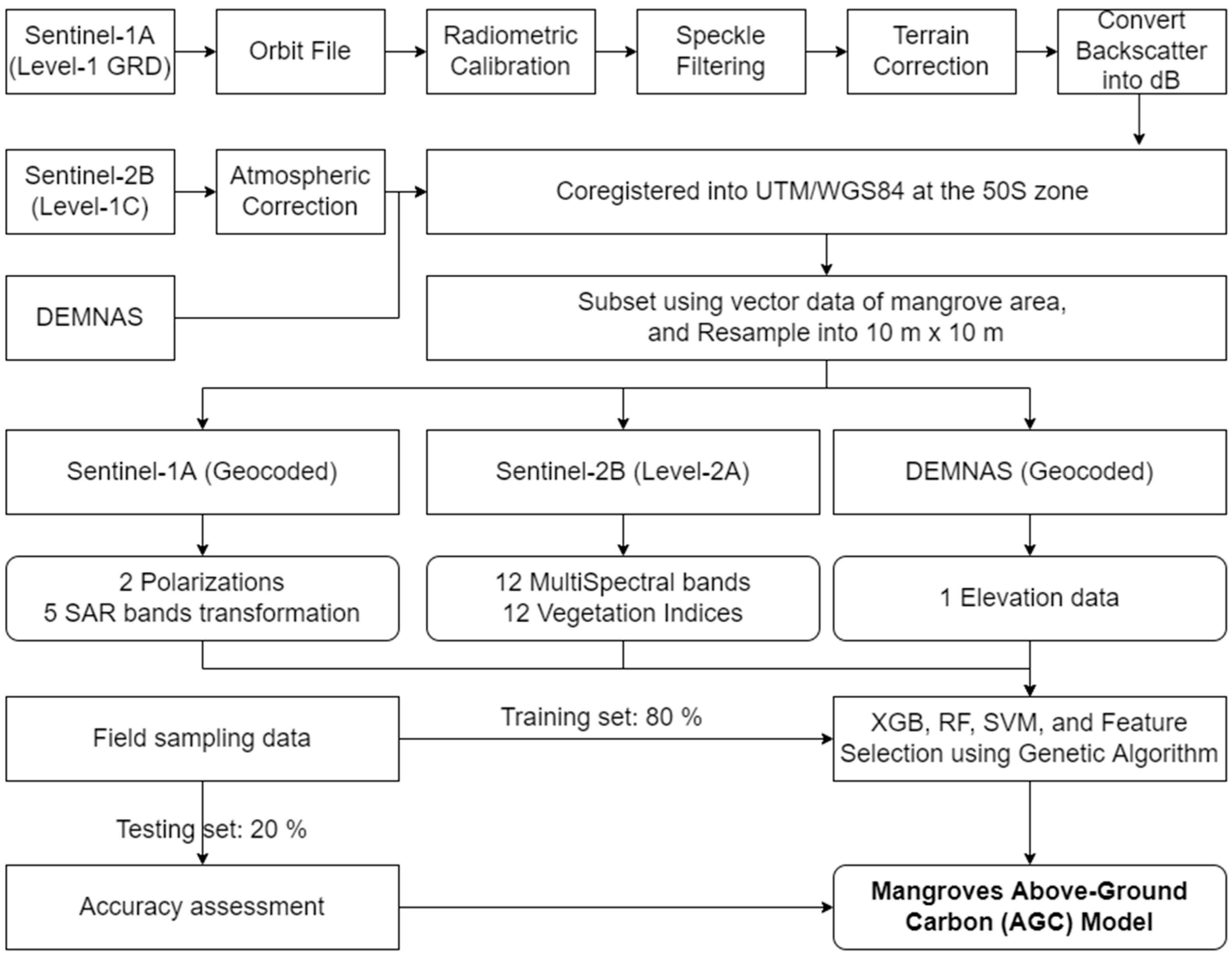
3.1. EO Image Processing

3.1.1. EO Image Pre-Processing

The S1A was processed in several steps, including applying the orbit file to update more accurately satellite orbit position, radiometric calibration to convert the intensity value of VV and VH into sigma nought (σ°), which can represent the actual backscatter of the object, speckle filtering to reduce the granular noise on the image, terrain correction to register the imagery from sensor geometry into the projection coordinate, and converting backscatter value into decibel (dB) units. The S2B level-1C already has the Top of Atmosphere (TOA) value and has been geometrically and radiometrically corrected [24]. To gain the Bottom of Atmospheric (BOA) reflectance (Level-2A), The S2B level-1C was converted using the Sen2Cor algorithm [22,35]. All the EO data (S1A, S2B, and DEMNAS) were clipped using the vector data of the mangrove area in Loh Buaya, co-registered into UTM/WGS84 at the 50S zone, and resampled into 10 m corresponds to the field plots size. According to Kamal [47], matching the size of plots with the image pixel resolution will improve the accuracy of mangrove identification. All data were processed using European Space Agency (ESA) SNAP software.

3.1.2. EO Image Transformations

Optical satellite imagery has been widely used to estimate mangrove carbon [16,48,49]. In tropical latitudes, minimum cloud coverage of optical imagery may be difficult to access. Therefore, previous studies have substituted optical imagery with SAR imagery for carbon estimation [50,51] or the combination of optical and SAR [22,52]. Further, a DEM may also be used to improve the accuracy of forest carbon estimates [53,54,55]. In this study, we employed a total of 32 variables consisting of 2 polarizations of S1A, 5 SAR bands transformations of S1A, 12 bands of S2B, 12 Vegetation Indices (VIs) of S2B, and an elevation model (DEMNAS) (Table 2). The SAR band transformations and VIs are sensitive to the plant and vegetation characteristics [16,56,57]. The total number of optimal inputs for predicting the AGC model was 12 variables composed of 5 VIs (NDVI, GNDVI, NDI45, SAVI, MCARI), the elevation model (DEMNAS), and 6 bands (B4, B5, B7, B8A, B11, and B12). The variables were normalized before further processing.

Table 2. Overview of variables used in this study.

3.2. Machine Learning Algorithms

3.2.1. Random Forest (RF)

The RF algorithm was developed by Breiman [72] for supervised classification and regression tasks, applying bootstrap sampling and bagging trees in the ensemble learning family. The RF model can effectively handle non-linear data without overestimation during the training and testing phases. In the RF model, approximately 2/3 of the total samples (in-bag) are used during the training phase and the remaining 1/3 of the total samples (out-of-bag, OOB) is used for the testing phase.

In the RF benchmark, a maximum depth, a minimum sample leaf, a minimum sample split, a maximum feature, and the number of trees as well as the number of features m can be tuned to fit a specific dataset. These parameters were optimized using five-fold cross-validation (CV) in the Python environment.

3.2.2. Support Vector Machine (SVM)

The SVM algorithm was developed by Vapnik [73] based on the statistical learning theory for supervised classification and regression tasks. This algorithm has been widely applied in numerous domains such as image processing, computer vision, pattern recognition, and environmental monitoring. In the SVM model, the choice of different kernel functions largely influences the model performance. For this reason, we selected the radial basis function (RBF) kernel in this work to minimize the bias as suggested by the prior studies for the estimates of mangrove AGC [52,74].

The effectiveness of the estimate of mangrove AGC can be highly influenced by the hyperparameters. In the SVM benchmark, we configured three main parameters with an RBF kernel: the regularization parameter (C), Epsilon (ε), and the kernel width (γ) using five-fold CV using Python scripting.

3.2.3. Extreme Gradient Boosting (XGB)

The XGB algorithm uses the theory of boosting technique and belongs to the ensemble-based decision tree learning. Initially introduced by Chen and Guestrin [75], XGB has been effectively applied in both classification and regression tasks for the supervised-learning domains [76].

In the XGB model, two regularization terms L₁ and L₂ are added to the cost functions to improve the generalization, optimize performance, and reduce the overfitting problem. In the XGB benchmark, several hyperparameters such as the booster, a maximum depth, a minimum child weight, several trees, and a learning rate must be set and tuned beforehand.

3.3. Model Configuration, Implementation, and Accuracy Assessment

3.3.1. Configuration and Training

A total of 50 samples were split randomly into the training set (80%) and the testing set (20%) of the total samples. The former set was used to construct the ML models using the features derived from multiple source EO such as bands’ reflectance, vegetation indices (VIs) derived from S2B, backscatters coefficients, and SAR transformation derived from S1A C-band as well as the national DEM, whereas the latter dataset was used to assess the predictive performance of the ML models. All features were normalized using the normalization function in the Scikit-learn library in Python 3.7 [77].

3.3.2. Hyperparameters Tuning

ML models consist of several parameters, which control the learning process during the construction of any ML model. These parameters are called hyperparameters, which often need to be tuned or optimized to achieve the highest regression performance. In this work, the hyperparameters of the RF, the SVM, and the XGB models were tuned and maintained during the training and the testing phases using a grid-search with a five-fold CV in the Scikit-learn library [77].

3.3.3. Feature Selection Using the Genetic Algorithm (GA)

In the current study, the GA was implemented in the Python environment to automatically select the optimal number of variables for estimating mangrove AGC in the study area. The GA adopts Darwinian natural selection theory to automatically tune the hyperparameters of an ML model [78]. In the GA, the vector of parameter values, which is called an individual, is the most important pattern to define a solution in each generation.

First, all features generated from S1A C-band SAR and S2B (input variables) were tested with the three ML models using a grid search with a five-fold CV to tune the hyperparameter of each model. Second, the highest predictive ML model performance for estimating mangrove AGC with the lowest root-mean-square error (RMSE) was chosen. The GA was then used in conjunction with the best predictive model to select the optimal features derived from the S2B MSI, VIs, and S1A, SAR transformations generated from S1A, and national DEM data for mangrove AGC estimation. Finally, all of the chosen ML models were tested with the best features for comparison.

3.3.4. Accuracy Assessment

We used several criteria including RMSE and the coefficient of determination (R²) for model evaluation and comparison of different ML algorithms for estimating mangrove AGC as they are well-known indices for assessing the performance of any regression model [52,79].

RMSE (Equation (3)) and R² (Equation (4)) are standard criteria for measuring errors of regression tasks, in which higher R² and lower RMSE values indicate the better regression model

RMSE = \sqrt{\sum_{i = 1}^{n} \frac{{({\hat{y}}_{i} - y_{i})}^{2}}{n}},

(3)

R^{2} = 1 - \frac{\sum_{i = 1}^{n} {(y_{i -} {\hat{y}}_{i})}^{2}}{\sum_{i = 1}^{n} {(y_{i -} \bar{y})}^{2}},

(4)

where

\hat{y}

_i and y_i are the estimated and measured mangrove AGC for the ith plot, respectively; n is the total number of sampling plots, and

\bar{y}

is the measured mean values of the mangrove AGC.

4. Results

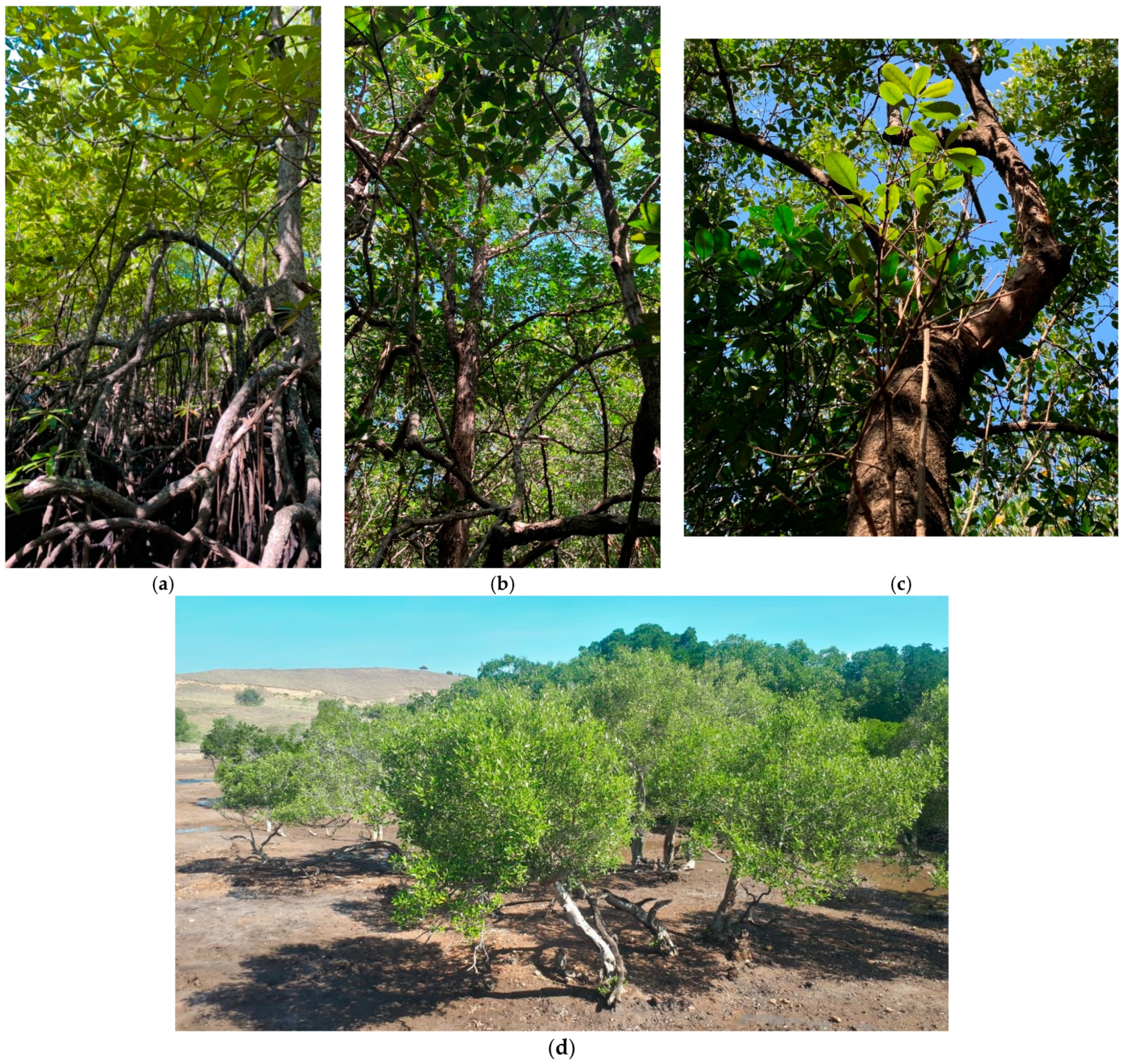
4.1. Characteristics of Mangrove Forests

Mangroves in the study area (Figure 3) also had varying DBH, ranging from 7.48 cm in plot 5 (Rhizophora apiculata) to 19.21 cm in plot 27 (Rhizophora mucronata) with an average of 12.67 cm. Based on the calculated results of AGC listed in Table 3, the lowest carbon stock was 13.63 Mg C ha⁻¹ in Plot 14 while the largest carbon stock was found in Plot 27 with 143.94 Mg C ha⁻¹. An average AGC was observed at approximately 57.51 Mg C ha⁻¹. The dominant species in the sampling plots were Rhizophora apiculata, which was common in 23 of the 50 plots. The calculation of carbon stock is influenced by DBH and wood density, therefore, although Rhizophora apiculata had the lowest DBH, this is not corresponding with the lowest carbon stock due to its wood density being higher than Ceriops decandra.

Figure 3. Mangrove species at study area: (a) Rhizophora apiculata, (b) Rhizophora mucronata, (c) Ceriops decandra, and (d) Lumnitzera racemosa. (Photos taken by Salma Noer ‘Aulia during field survey).

Table 3. Identification of mangrove characteristics in the study area.

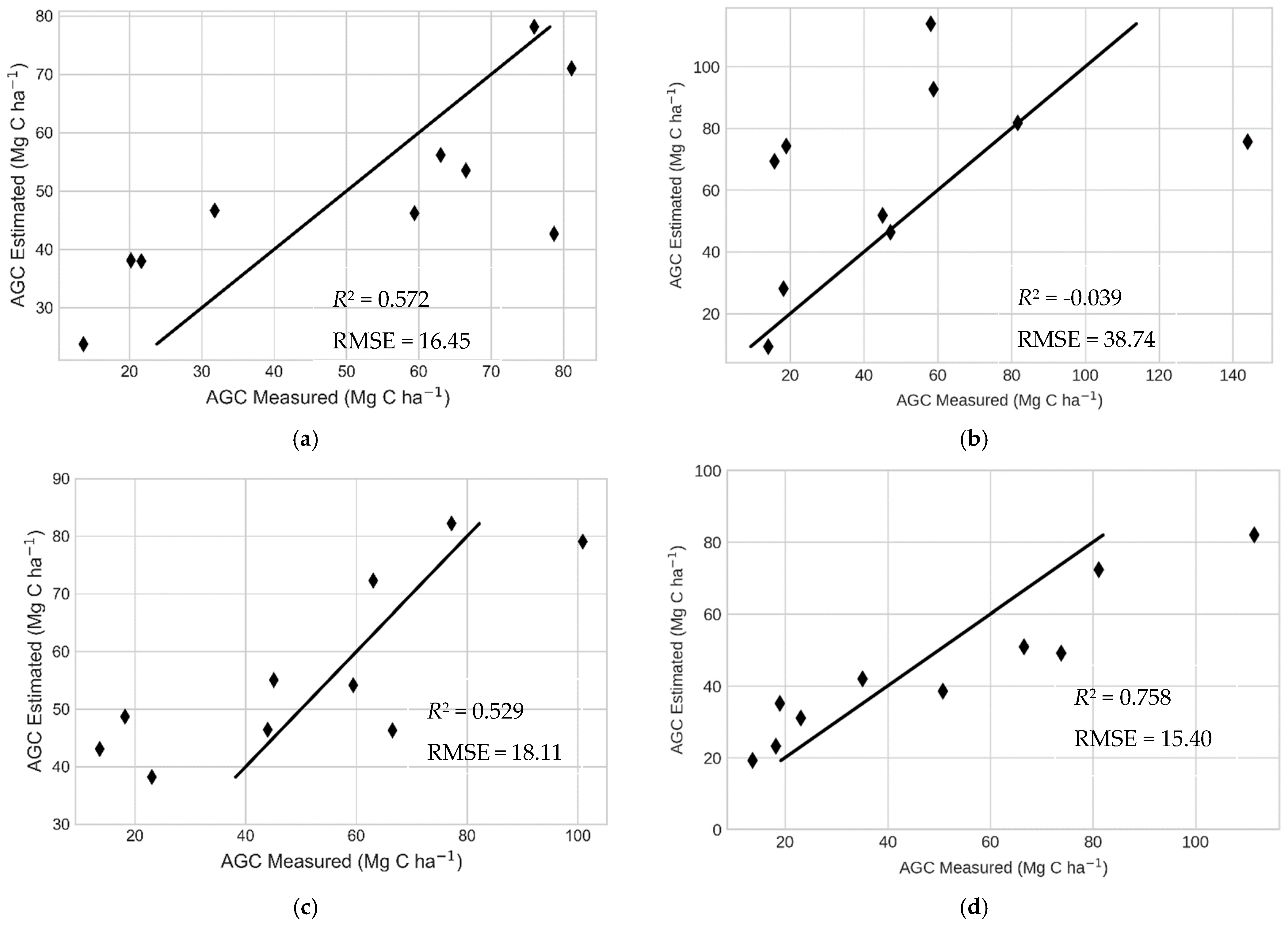
4.2. Model Performance and Comparison

Table 4 and Figure 4 compare the model performance of the three ML techniques with all input variables derived from S2B MSI, VIs, and S1A together with SAR transformation as well as DEM and the proposed hybrid XGB-GA model with the optimal 12 features. The hybrid model XGB-GA yielded the highest performance in both the training phase (R² = 0.857) and the testing phase (R² = 0.758) and had an RMSE = 15.40 Mg C ha⁻¹ for mangrove AGC estimation in the study site. The XGB-GA model incorporating the S2B (6 MS bands), and VIs (5 bands) together with DEM data achieved the highest performance, reflecting a good fit between the model estimates and field-based measurements. The next-highest performers in the testing phase were the XGB (R² = 0.572) and the RF (R² = 0.529) models. In contrast, the SVM model (R² testing = −0.039) was unsuitable for estimating the mangrove AGC at Loh Buaya (Table 4).

Table 4. Performance comparison of ML techniques on mangrove AGC estimation (bold values highlight the best-performing model).

Figure 4. Scatter plots of the estimated (Y-axis) and measured (X-axis) mangrove AGC in the three ML models and the proposed hybrid XGB-GA model (a) XGB, (b) SVM, (c) RF, (d) XGB-GA.

Table 5 compares the effectiveness and performances of the XGB-GA model in four scenarios (SC) for mangrove AGC estimation using difference integrations of S2B, S1A, VIs, SAR transformations, and DEM data. The XGB-GA models using the different combinations of datasets had promising results in both four SC with the R² greater than 0.57 in the testing phase. The XGB optimized by the GA with 12 optimal features in SC3 produced the best accuracy with the highest R² of 0.758 and the lowest RMSE of 15.40 Mg C ha⁻¹ as well as reduced overfitting problems in both the training and the testing phases.

Table 5. Performance of the XGB-GA model using different numbers of variables (bold values highlight the best-performing model).

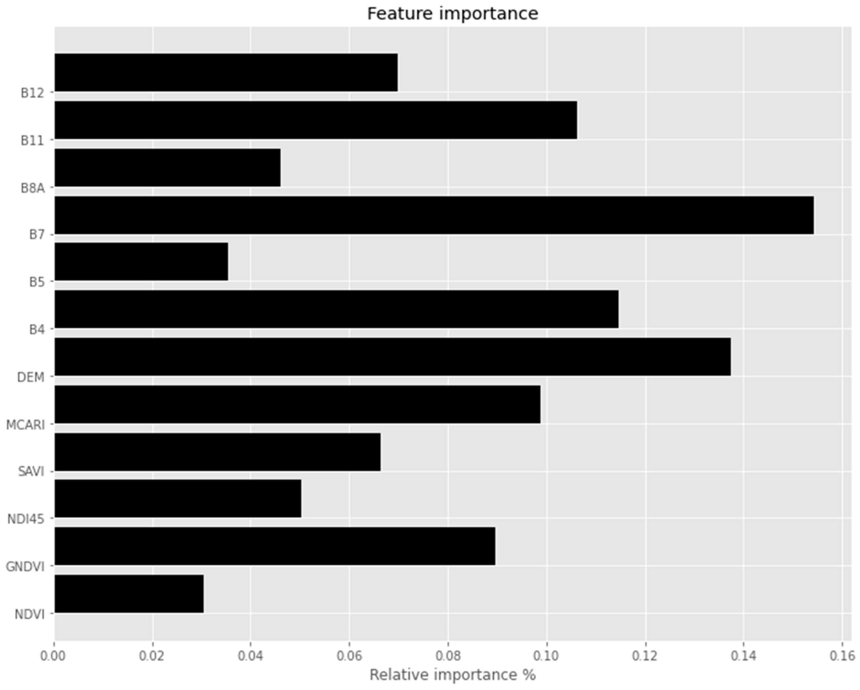
4.3. The Important Variables

Among the 12 multispectral bands of S2B, the Red Edge-3 (Band 7 at 779.7 nm), and the Red (Band 4 at 664.9 nm) were the most sensitive to mangrove AGC in the current study, followed by the two SWIR spectra (band 11 at 1610.4 nm and band 12 at 2185.7 nm). Interestingly, among the 12 VI indices, the Modified Chlorophyll Absorption in Reflectance Index (MCARI) and the Green Normalized Difference Vegetation Index (GNDVI) were also important variables for estimating mangrove AGC in the study area, followed by the Soil-Adjusted Vegetation Index (SAVI) and the Normalized Difference Index (NDI45) (bands 4 and 5 of S2B) (see Figure 5). The DEM data showed that mangrove AGC was sensitive to elevation. It is noted that the VH and VV backscatter coefficients of the S1A C-band and their SAR transformations were likely less important and were eliminated in the final optimal 12 features selection using the GA algorithm (Figure 5).

Figure 5. Variable importance of the optimal 12 features for mangrove AGC estimates.

4.4. Mangroves AGC Models

The prediction performance of the XGB-GA model for estimating mangrove AGC was improved by combining the S2B multispectral bands, VIs, and DEM datasets. Thus, the hybrid XGB-GA model was employed for generating mangrove AGC in the study area. The final results were computed to a raster in GeoTiff format for visualization. The AGC map was interpreted (Figure 6), showing the mangrove AGC ranging from 2.52 to 123.89 Mg C ha⁻¹ (average = 57.16 Mg C ha⁻¹).

Figure 6. Spatial distribution of mangrove AGC at Loh Buaya.

5. Discussion

Rhizophora was the dominant genus in the study area, in common with other Indonesian mangroves forests at Karimun Jawa island [80,81], Bali island [82], and East Java [83], and is the dominant tropical genus [84]. Besides Rhizophora sp., other important species found in the study area included Ceriops decandra and Lumnitzera racemosa, their first observation in the area (c.f. Erdmann [37] and Suraji et al. [38]. The estimation of AGC calculation was controlled by tree density and girth [16,85], and also wood density [86]. Canopy cover provided a negligible contribution to biomass, though is likely to be sensitive to variation in hydroperiod [17] and influence forest productivity.

Our results show that the XGBR-GA model yielded the highest performance in the estimation of mangrove AGC, with an R² and an RMSE of 0.758 and 15.40 Mg C ha⁻¹, respectively. The lowest performing model was SVM, with an R² and an RMSE of −0.039 and 38.74 Mg C ha⁻¹. Both the XGB model (R² = 0.572) and the RF model (R² = 0.529) produced a relatively good performance for the estimates of mangrove AGC, indicating that the ensemble decision trees regression models were suitable for mapping mangrove AGC. As shown in Table 4 and Table 5, the combined S2B and VIs as well as DEM data significantly improved the estimation of mangrove AGC in the study area. Backscatter coefficients and transformations generated from the dual polarimetric VV and VH of the S1A C-band were less important. These results are strongly consistent with a recent study in Northern Vietnam [35] and prove that the ML approach can also depict mangrove biomass/carbon with satisfying results compared to conventional parametric regression models. This is due to the ability to provide nearly unbiased error prediction and select effective variables [87,88]. Overall, the XGB-GA model performed well and outperformed the existing algorithms for estimating mangrove AGC in an Indonesian mangrove national park. Indonesian Government through the Ministry of Environment and Forestry has released an operational plan for FOLU (Forestry and Other Land Use) Net Sink to reduce greenhouse emission in 2030 [89] and mangrove has been mentioned for their potential for carbon absorption ability. Therefore, this study could potentially support that policy using a state-of-the-art and scientific approach.

The XGB-GA model estimated the mangrove AGC at Loh Buaya ranging from 2.52 to 123.89 Mg C ha⁻¹ with a mean of 57.16 Mg C ha⁻¹. These numbers fit well a range between 13.63 and 143.94 Mg C ha⁻¹ with a mean measured mangrove AGC of 57.32 Mg C ha⁻¹ (Table 3). In comparison to existing global coarse (30 m) mangrove biomass datasets [90], the results of this study produced a more suitable AGC range corresponding to field AGC data, with promising R2 and RMSE values. More accurate information on mangrove biomass is frequently produced by higher satellite spatial resolution [91]. This finding is consistent with the finding of Nguyen [92], who compared the ability of Sentinel-2 and Landsat-8 to map the AGB of mangroves in Vietnam. However, the proposed hybrid model was likely under-estimating at high observed carbon values and over-estimating at low observed carbon values. The scatterplot in Figure 4d depicts the prediction ability of the proposed hybrid XGB-GA model with optimal features to estimate the AGC of mangrove forests ranging from 10 to 100 Mg C ha⁻¹ with the highest accuracy between 20 and 80 Mg C ha⁻¹. One possible reason could be the saturation levels for mangrove AGC estimates of S2B data, resulting in weak prediction performance at high AGC values and dense mangrove canopy densities observed in Indonesian mangrove ecosystems as reported by [88]. Further research focuses on the data integration and fusion between multispectral and longer wavelength SAR sensors, particularly integrating S2B and ALOS-2 PALSAR-2 to overcome the limitation saturation problem of the S2B sensor.

The results of variable importance in Figure 5 showed that the mangrove AGC at the Loh Buaya in Indonesia was largely retrieved from the Red band and the Red Edge bands. A similar observation was reported in other mangrove regions in Southeast Asian nations [87,93]. The Red and the Red Edge, and SWIR reflectance are more sensitive indicators to mangrove carbon stock volume than the visible reflectance [94]. Our results also revealed that the new vegetation index NDI45, which is generated from bands 4 and 5 of the S2B sensor, is probably correlated with mangrove AGC. The two SWIR spectra (bands 11 and 12) as well as the narrow NIR (band 8A) also play a vital role in estimating mangrove AGC. Noticeably, the MCARI derived from S2B was strongly correlated with mangrove AGC in the national park. The high quality of a national DEM also contributes to the hybrid ML model as it is strongly related to the distribution of mangrove canopy cover as shown in a recent study [17]. Furthermore, this is the first use of the national DEM for mangrove AGC estimation, though it is commonly used for disaster-related mapping, e.g., tsunami and tidal flood [95,96].

6. Conclusions

We incorporated S2B and S1A together with national DEM data into the XGB-GA model to estimate the mangrove AGC in an Indonesian mangrove area for the first time. The XGB-GA model outperformed other well-known ML models in mangrove AGC retrieval at Loh Buaya. The proposed hybrid XGB-GA with 12 optimal features estimated the mangrove AGC with the highest prediction accuracy for the first time in the Indonesian mangrove ecosystems (R² = 0.758, RMSE = 15.40 Mg C ha⁻¹). Interestingly, we found that new vegetation indices derived from the S2B data, such as the Normalized Difference Index (NDI45) and the Modified Chlorophyll Absorption in Reflectance Index (MCARI) were sensitively detected mangrove AGC in the Indonesian mangrove ecosystem.

Author Contributions

Conceptualization, S.S.R. and T.D.P.; methodology, S.S.R. and T.D.P.; software, S.S.R. and T.D.P.; validation, S.S.R. and T.D.P.; formal analysis, S.S.R. and T.D.P.; investigation, T.D.P. and S.N.; resources, S.N.; data curation, T.D.P. and S.N.; writing—original draft preparation, S.S.R. and T.D.P.; writing—review and editing, S.S.R., T.D.P. and N.S.; visualization, S.S.R. and T.D.P.; supervision, S.S.R. and M.I.P.; project administration, S.S.R. and S.N.; funding acquisition, S.S.R. All authors have read and agreed to the published version of the manuscript.

Funding

This research was funded by Badan Penelitian dan Pengabdian Masyarakat (BPPM), FPIK Universitas Brawijaya through the scheme of Hibah Penelitian Dosen (Lecturer Research Grant) contract number 4717/UN10.F06/KS/2022.

Data Availability Statement

Not Applicable.

Acknowledgments

T.D.P. is supported by a Macquarie University Research Fellowship (Grant No. MQRF0001124-2021). The authors would like to thank local authorities for their generous assistance during the fieldwork and technical data process.

Conflicts of Interest

The authors declare no conflict of interest.

References

Kumari, A.; Rathore, M.S. Roles of Mangroves in Combating the Climate Change. In Mangroves: Ecology, Biodiversity and Management; Rastogi, R.P., Phulwaria, M., Gupta, D.K., Eds.; Springer Singapore: Gateway East, Singapore, 2021; pp. 225–255. ISBN 978-981-16-2494-0. [Google Scholar]
Hu, T.; Zhang, Y.Y.; Su, Y.; Zheng, Y.; Lin, G.; Guo, Q. Mapping the global mangrove forest aboveground biomass using multisource remote sensing data. Remote Sens. 2020, 12, 1690. [Google Scholar] [CrossRef]
Mumby, P.J.; Edwards, A.J.; Ernesto Arias-González, J.; Lindeman, K.C.; Blackwell, P.G.; Gall, A.; Gorczynska, M.I.; Harborne, A.R.; Pescod, C.L.; Renken, H.; et al. Mangroves enhance the biomass of coral reef fish communities in the Caribbean. Nature 2004, 427, 533–536. [Google Scholar] [CrossRef]
Buelow, C.; Sheaves, M. A birds-eye view of biological connectivity in mangrove systems. Estuar. Coast. Shelf Sci. 2015, 152, 33–43. [Google Scholar] [CrossRef]
Hernández-Blanco, M.; Costanza, R.; Cifuentes-Jara, M. Economic valuation of the ecosystem services provided by the mangroves of the Gulf of Nicoya using a hybrid methodology. Ecosyst. Serv. 2021, 49, 101258. [Google Scholar] [CrossRef]
Marlianingrum, P.R.; Kusumastanto, T.; Adrianto, L.; Fahrudin, A. Valuing habitat quality for managing mangrove ecosystem services in coastal Tangerang District, Indonesia. Mar. Policy 2021, 133, 104747. [Google Scholar] [CrossRef]
Goldberg, L.; Lagomasino, D.; Thomas, N.; Fatoyinbo, T. Global declines in human-driven mangrove loss. Glob. Chang. Biol. 2020, 26, 5844–5855. [Google Scholar] [CrossRef]
Fauzi, A.; Sakti, A.; Yayusman, L.; Harto, A.; Prasetyo, L.; Irawan, B.; Kamal, M.; Wikantika, K. Contextualizing mangrove forest deforestation in southeast asia using environmental and socio-economic data products. Forests 2019, 10, 952. [Google Scholar] [CrossRef]
Latiff, A.; Faridah-Hanum, I. Mangrove Ecosystem of Malaysia: Status, Challenges and Management Strategies. In Mangrove Ecosystems of Asia; Faridah-Hanum, I., Latiff, A., Hakeem, K.R., Ozturk, M., Eds.; Springer New York: New York, NY, USA, 2014; pp. 1–22. ISBN 978-1-4614-8582-7. [Google Scholar]
Pendleton, L.; Donato, D.C.; Murray, B.C.; Crooks, S.; Jenkins, W.A.; Sifleet, S.; Craft, C.; Fourqurean, J.W.; Kauffman, J.B.; Marbà, N.; et al. Estimating Global “Blue Carbon” Emissions from Conversion and Degradation of Vegetated Coastal Ecosystems. PLoS ONE 2012, 7, e43542. [Google Scholar] [CrossRef]
Hutchison, J.; Manica, A.; Swetnam, R.; Balmford, A.; Spalding, M. Predicting Global Patterns in Mangrove Forest Biomass. Conserv. Lett. 2014, 7, 233–240. [Google Scholar] [CrossRef]
Hagger, V.; Worthington, T.A.; Lovelock, C.E.; Adame, M.F.; Amano, T.; Brown, B.M.; Friess, D.A.; Landis, E.; Mumby, P.J.; Morrison, T.H.; et al. Drivers of global mangrove loss and gain in social-ecological systems. Nat. Commun. 2022, 13, 6373. [Google Scholar] [CrossRef]
Friess, D.A.; Yando, E.S.; Abuchahla, G.M.O.; Adams, J.B.; Cannicci, S.; Canty, S.W.J.; Cavanaugh, K.C.; Connolly, R.M.; Cormier, N.; Dahdouh-Guebas, F.; et al. Mangroves give cause for conservation optimism, for now. Curr. Biol. 2020, 30, R153–R154. [Google Scholar] [CrossRef]
Sani, D.A.; Hashim, M.; Hossain, M.S. Remote sensing models used for mapping and estimation of blue carbon biomass in seagrass-mangrove habitats: A review. In Proceedings of the 39th Asian Conference on Remote Sensing (ACRS), Renaissance Kuala Lumpur Hotel, Lumpur, Malaysia, 15–19 October 2018; Volume 1, pp. 399–408. [Google Scholar]
Lamont, K.; Saintilan, N.; Kelleway, J.J.; Mazumder, D.; Zawadzki, A. Thirty-Year Repeat Measures of Mangrove Above- and Below-Ground Biomass Reveals Unexpectedly High Carbon Sequestration. Ecosystems 2020, 23, 370–382. [Google Scholar] [CrossRef]
Purnamasari, E.; Kamal, M.; Wicaksono, P. Comparison of vegetation indices for estimating above-ground mangrove carbon stocks using PlanetScope image. Reg. Stud. Mar. Sci. 2021, 44, 101730. [Google Scholar] [CrossRef]
Saintilan, N.; Lymburner, L.; Wen, L.; Haigh, I.D.; Ai, E.; Kelleway, J.J.; Rogers, K.; Pham, T.D.; Lucas, R. The lunar nodal cycle controls mangrove canopy cover on the Australian continent. Sci. Adv. 2022, 8, eabo6602. [Google Scholar] [CrossRef]
Jones, A.R.; Raja Segaran, R.; Clarke, K.D.; Waycott, M.; Goh, W.S.H.; Gillanders, B.M. Estimating Mangrove Tree Biomass and Carbon Content: A Comparison of Forest Inventory Techniques and Drone Imagery. Front. Mar. Sci. 2020, 6, 784. [Google Scholar] [CrossRef]
Tran, T.V.; Reef, R.; Zhu, X. A Review of Spectral Indices for Mangrove Remote Sensing. Remote Sens. 2022, 14, 4868. [Google Scholar] [CrossRef]
Pham, T.D.; Xia, J.; Ha, N.T.; Bui, D.T.; Le, N.N.; Tekeuchi, W. A Review of Remote Sensing Approaches for Monitoring Blue Carbon Ecosystems: Mangroves, Seagrasses and Salt Marshes during 2010–2018. Sensors 2019, 19, 1933. [Google Scholar] [CrossRef]
Wang, L.; Jia, M.; Yin, D.; Tian, J. A review of remote sensing for mangrove forests: 1956–2018. Remote Sens. Environ. 2019, 231, 111223. [Google Scholar] [CrossRef]
Nuthammachot, N.; Askar, A.; Stratoulias, D.; Wicaksono, P. Combined use of Sentinel-1 and Sentinel-2 data for improving above-ground biomass estimation. Geocarto Int. 2020, 37, 366–376. [Google Scholar] [CrossRef]
USGS. Imagery for Everyone… Timeline Set to Release Entire USGS Landsat Archive at No Charge. 2008. Available online: https://www.usgs.gov/media/files/2008-imagery-everyonetimeline-set-release-entire-usgs-landsat-0 (accessed on 1 November 2022).
European Space Agency. Sentinel-2 MSI—Technical Guide—Sentinel Online 2019. Available online: https://sentinels.copernicus.eu/web/sentinel/technical-guides/sentinel-2-msi (accessed on 5 September 2022).
European Space Agency. Sentinel-1 SAR User Guide. 2013. Available online: https://sentinel.esa.int/web/sentinel/user-guides/sentinel-1-sar (accessed on 1 November 2022).
Bunting, P.; Rosenqvist, A.; Hilarides, L.; Lucas, R.M.; Thomas, N.; Tadono, T.; Worthington, T.A.; Spalding, M.; Murray, N.J. Global Mangrove Extent Change 1996–2020: Global Mangrove Watch Version 3.0. Remote Sens. 2022, 14, 3657. [Google Scholar] [CrossRef]
Lagomasino, D.; Fatoyinbo, T.; Lee, S.; Feliciano, E.; Trettin, C.; Shapiro, A.; Mangora, M.M. Measuring mangrove carbon loss and gain in deltas. Environ. Res. Lett. 2019, 14, 25002. [Google Scholar] [CrossRef]
Liu, X.; Fatoyinbo, T.E.; Thomas, N.M.; Guan, W.W.; Zhan, Y.; Mondal, P.; Lagomasino, D.; Simard, M.; Trettin, C.C.; Deo, R.; et al. Large-Scale High-Resolution Coastal Mangrove Forests Mapping Across West Africa With Machine Learning Ensemble and Satellite Big Data. Front. Earth Sci. 2021, 8, 560933. [Google Scholar] [CrossRef]
Sidhu, N.; Pebesma, E.; Câmara, G. Using Google Earth Engine to detect land cover change: Singapore as a use case. Eur. J. Remote Sens. 2018, 51, 486–500. [Google Scholar] [CrossRef]
Nemani, R.; Votava, P.; Michaelis, A.; Melton, F.; Milesi, C. Collaborative Supercomputing for Global Change Science. Eos Trans. Am. Geophys. Union 2011, 92, 109–116. [Google Scholar] [CrossRef]
Argamosa, R.J.; Blanco, A.C.; Baloloy, A.B.; Candido, C.G.; Dumalag, J.B.; DImapilis, L.L.; Paringit, E.C. Modelling above Ground Biomass of Mangrove Forest Using Sentinel-1 Imagery. ISPRS Ann. Photogramm. Remote Sens. Spat. Inf. Sci. 2018, 4, 13–20. [Google Scholar] [CrossRef]
Diniz, C.; Cortinhas, L.; Nerino, G.; Rodrigues, J.; Sadeck, L.; Adami, M.; Souza-Filho, P.W.M. Brazilian Mangrove Status: Three Decades of Satellite Data Analysis. Remote Sens. 2019, 11, 808. [Google Scholar] [CrossRef]
Pham, T.D.; Le, N.N.; Ha, N.T.; Nguyen, L.V.; Xia, J.; Yokoya, N.; To, T.T.; Trinh, H.X.; Kieu, L.Q.; Takeuchi, W. Estimating mangrove above-ground biomass using extreme gradient boosting decision trees algorithm with fused sentinel-2 and ALOS-2 PALSAR-2 data in can Gio biosphere reserve, Vietnam. Remote Sens. 2020, 12, 777. [Google Scholar] [CrossRef]
Tian, Y.; Huang, H.; Zhou, G.; Zhang, Q.; Tao, J.; Zhang, Y.; Lin, J. Aboveground mangrove biomass estimation in Beibu Gulf using machine learning and UAV remote sensing. Sci. Total Environ. 2021, 781, 146816. [Google Scholar] [CrossRef]
Pham, T.D.; Yokoya, N.; Xia, J.; Ha, N.T.; Le, N.N.; Nguyen, T.T.T.; Dao, T.H.; Vu, T.T.P.; Pham, T.D.; Takeuchi, W. Comparison of machine learning methods for estimating mangrove above-ground biomass using multiple source remote sensing data in the red river delta biosphere reserve, Vietnam. Remote Sens. 2020, 12, 1334. [Google Scholar] [CrossRef]
UNESCO. Komodo National Park—UNESCO World Heritage Centre 2014. Available online: http://whc.unesco.org/en/list/685 (accessed on 3 November 2022).
Erdmann, A.M. A Natural History Guide to Komodo National Park; The Nature Conservancy: Virginia, UK, 2004; p. 198. [Google Scholar]
Suraji, S.; Hasan, S.; Suharyanto, S.; Yonvitner, Y.; Koeshendrajana, S.; Prasetiyo, D.E.; Widianto, A.; Dermawan, A. Nilai Penting Dan Strategis Nasional Rencana Zonasi Kawasan Taman Nasional Komodo. J. Sos. Ekon. Kelaut. dan Perikan. 2020, 15, 15–32. [Google Scholar] [CrossRef]
Dharmawan, I.W.E.; Suyarso; Yaya, I.U.; Prayudha, B.; Pramudji. Panduan Monitoring Struktur Komunitas Mangrove Di Indonesia, 1st ed.; Media Sains Nasional: Bogor, Indonesia, 2020; ISBN 9786239430603. [Google Scholar]
Dharmawan, I.W.; Sastrosuwondo, P. Panduan Monitoring Status Ekosistem Mangrove di Indonesia; COREMAP CITI LIPI: Jakarta, Indonesia, 2014. [Google Scholar]
Komiyama, A.; Poungparn, S.; Kato, S. Common allometric equations for estimating the tree weight of Common allometric equations for estimating the tree weight of mangroves. J. Trop. Ecol. 2005, 21, 471–477. [Google Scholar] [CrossRef]
World Agroforestry. ICRAF Database—Wood Density. 2016. Available online: http://db.worldagroforestry.org/wd (accessed on 5 October 2022).
Badan Standar Nasional. Pengukuran dan Penghitungan Cadangan Karbon—Pengukuran Lapangan untuk Penaksiran Cadangan Karbon Hutan (Ground Based Forest Carbon Accounting); BSNI: Jakarta, Indonesia, 2011. [Google Scholar]
European Space Agency. User Guides—Sentinel-1 SAR—Polarimetry—Sentinel Online. 2022. Available online: https://sentinels.copernicus.eu/web/sentinel/user-guides/sentinel-1-sar/product-overview/polarimetry (accessed on 5 November 2022).
Badan Informasi Geospasial (BIG)/Indonesian Geospatial Information Agency. DEMNAS. 2022. Available online: https://tanahair.indonesia.go.id/demnas/#/demnas (accessed on 5 October 2022).
Susetyo, D.B.; Lumban-Gaol, Y.A.; Sofian, I. Prototype of national digital elevation model in Indonesia. Int. Arch. Photogramm. Remote Sens. Spat. Inf. Sci.—ISPRS Arch. 2018, 42, 687–692. [Google Scholar] [CrossRef]
Kamal, M.; Phinn, S.; Johansen, K. Assessment of multi-resolution image data for mangrove leaf area index mapping. Remote Sens. Environ. 2016, 176, 242–254. [Google Scholar] [CrossRef]
Wicaksono, P. Mangrove above-ground carbon stock mapping of multi-resolution passive remote-sensing systems. Int. J. Remote Sens. 2017, 38, 1551–1578. [Google Scholar] [CrossRef]
Wicaksono, P.; Danoedoro, P.; Hartono, H.; Nehren, U.; Ribbe, L. Preliminary work of mangrove ecosystem carbon stock mapping in small island using remote sensing: Above and below ground carbon stock mapping on medium resolution satellite image. Remote Sens. Agric. Ecosyst. Hydrol. XIII 2011, 8174, 81741B. [Google Scholar] [CrossRef]
Thapa, R.B.; Watanabe, M.; Motohka, T.; Shimada, M. Potential of high-resolution ALOS–PALSAR mosaic texture for aboveground forest carbon tracking in tropical region. Remote Sens. Environ. 2015, 160, 122–133. [Google Scholar] [CrossRef]
Nesha, M.K.; Hussin, Y.A.; van Leeuwen, L.M.; Sulistioadi, Y.B. Modeling and mapping aboveground biomass of the restored mangroves using ALOS-2 PALSAR-2 in East Kalimantan, Indonesia. Int. J. Appl. Earth Obs. Geoinf. 2020, 91, 102158. [Google Scholar] [CrossRef]
Pham, T.D.; Yoshino, K.; Le, N.N.; Bui, D.T. Estimating aboveground biomass of a mangrove plantation on the Northern coast of Vietnam using machine learning techniques with an integration of ALOS-2 PALSAR-2 and Sentinel-2A data. Int. J. Remote Sens. 2018, 39, 7761–7788. [Google Scholar] [CrossRef]
Stovall, A.E.L.; Fatoyinbo, T.; Thomas, N.M.; Armston, J.; Ebanega, M.O.; Simard, M.; Trettin, C.; Obiang Zogo, R.V.; Aken, I.A.; Debina, M.; et al. Comprehensive comparison of airborne and spaceborne SAR and LiDAR estimates of forest structure in the tallest mangrove forest on earth. Sci. Remote Sens. 2021, 4, 100034. [Google Scholar] [CrossRef]
Lucas, R.; Van De Kerchove, R.; Otero, V.; Lagomasino, D.; Fatoyinbo, L.; Omar, H.; Satyanarayana, B.; Dahdouh-Guebas, F. Structural characterisation of mangrove forests achieved through combining multiple sources of remote sensing data. Remote Sens. Environ. 2020, 237, 111543. [Google Scholar] [CrossRef]
Maeda, Y.; Fukushima, A.; Imai, Y.; Tanahashi, Y.; Nakama, E.; Ohta, S.; Kawazoe, K.; Akune, N. Estimating carbon stock changes of mangrove forests using satellite imagery and airborne LiDAR data in the South Sumatra state, Indonesia. Int. Arch. Photogramm. Remote Sens. Spat. Inf. Sci.—ISPRS Arch. 2016, 41, 705–709. [Google Scholar] [CrossRef]
Jin, Z.; Azzari, G.; You, C.; Di Tommaso, S.; Aston, S.; Burke, M.; Lobell, D.B. Smallholder maize area and yield mapping at national scales with Google Earth Engine. Remote Sens. Environ. 2019, 228, 115–128. [Google Scholar] [CrossRef]
Schulz, D.; Yin, H.; Tischbein, B.; Verleysdonk, S.; Adamou, R.; Kumar, N. Land use mapping using Sentinel-1 and Sentinel-2 time series in a heterogeneous landscape in Niger, Sahel. ISPRS J. Photogramm. Remote Sens. 2021, 178, 97–111. [Google Scholar] [CrossRef]
Hajduch, G.; Bourbigot, M.; Johnsen, H.; Piantanida, R. Sentinel-1 User Handbook. 2022. Available online: https://sentinel.esa.int/documents/247904/1877131/Sentinel-1-Product-Specification-18052021.pdf (accessed on 10 November 2022).
Simental, E.; Verner Guthrie, M.; Scientist Bruce Blundell, P.S. Polarimetry Band Ratios, Decompositions, and Statistics for Terrain Characterization. In Global Priorities in Land Remote Sensing, Proceedings of the Pecora 16, Sioux Falls, South Dakota, 23–27 October 2005; American Society for Photogrammetry and Remote Sensing: Bethesda, MD, USA, 2005. [Google Scholar]
Nasonova, S.; Scharien, R.; Geldsetzer, T.; Howell, S.; Power, D. Optimal Compact Polarimetric Parameters and Texture Features for Discriminating Sea Ice Types during Winter and Advanced Melt. Can. J. Remote Sens. 2019, 44, 390–411. [Google Scholar] [CrossRef]
Baronti, S.; Carla, R.; Sigismondi, S.; Alparone, L. Principal component analysis for change detection on polarimetric multitemporal SAR data. In Proceedings of the IGARSS’94—1994 IEEE International Geoscience and Remote Sensing Symposium, Pasadena, CA, USA, 8–12 August 1994; Volume 4, pp. 2152–2154. [Google Scholar] [CrossRef]
European Space Agency. Sentinel-2 User Handbook. 2015. Available online: https://sentinels.copernicus.eu/web/sentinel/user-guides/document-library/-/asset_publisher/xlslt4309D5h/content/sentinel-2-user-handbook (accessed on 15 November 2022).
Jordan, C.F. Derivation of Leaf-Area Index from Quality of Light on the Forest Floor. Ecology 1969, 50, 663–666. [Google Scholar] [CrossRef]
Tucker, C.J. Red and photographic infrared linear combinations for monitoring vegetation. Remote Sens. Environ. 1979, 8, 127–150. [Google Scholar] [CrossRef]
Candiago, S.; Remondino, F.; De Giglio, M.; Dubbini, M.; Gattelli, M. Evaluating Multispectral Images and Vegetation Indices for Precision Farming Applications from UAV Images. Remote Sens. 2015, 7, 4026–4047. [Google Scholar] [CrossRef]
Soria, J.; Ruiz, M.; Morales, S. Monitoring Subaquatic Vegetation Using Sentinel-2 Imagery in Gallocanta Lake (Aragón, Spain). Earth 2022, 3, 363–382. [Google Scholar] [CrossRef]
Huete, A.R. A soil-adjusted vegetation index (SAVI). Remote Sens. Environ. 1988, 25, 295–309. [Google Scholar] [CrossRef]
Gómez-Giráldez, P.J.; Pérez-Palazón, M.J.; Polo, M.J.; González-Dugo, M.P. Monitoring grass phenology and hydrological dynamics of an oak-grass savanna ecosystem using sentinel-2 and terrestrial photography. Remote Sens. 2020, 12, 600. [Google Scholar] [CrossRef]
Daughtry, C.S.T.; Walthall, C.L.; Kim, M.S.; de Colstoun, E.B.; McMurtrey, J.E. Estimating Corn Leaf Chlorophyll Concentration from Leaf and Canopy Reflectance. Remote Sens. Environ. 2000, 74, 229–239. [Google Scholar] [CrossRef]
Qi, J.; Chehbouni, A.; Huete, A.R.; Kerr, Y.H.; Sorooshian, S. A modified soil adjusted vegetation index. Remote Sens. Environ. 1994, 48, 119–126. [Google Scholar] [CrossRef]
Richardson, A.J.; Wiegand, C.L. Distinguishing vegetation from soil background information. Photogramm. Eng. Remote Sensing 1977, 43, 1541–1552. [Google Scholar]
Breiman, L. Random Forests. Mach. Learn. 2001, 45, 5–32. [Google Scholar] [CrossRef]
Vapnik, V.N. An overview of statistical learning theory. IEEE Trans. Neural Networks 1999, 10, 988–999. [Google Scholar] [CrossRef] [PubMed]
Pham, T.D.; Yoshino, K.; Bui, D.T. Biomass estimation of Sonneratia caseolaris (l.) Engler at a coastal area of Hai Phong city (Vietnam) using ALOS-2 PALSAR imagery and GIS-based multi-layer perceptron neural networks. GIScience Remote Sens. 2017, 54, 329–353. [Google Scholar] [CrossRef]
Chen, T.; Guestrin, C. XGBoost: A Scalable Tree Boosting System. In KDD’16, Proceedings of the 22nd ACM SIGKDD International Conference on Knowledge Discovery and Data Mining, San Francisco, CA, USA, 13–17 August 2016; Association of Computing Machinery: New York, NY, USA, 2016. [Google Scholar]
Nielsen, D. Tree Boosting With XGBoost Why Does XGBoost Win “Every” Machine Learning Competition? Master’s Thesis, NTNU: Norwegian University of Science and Trcnology, Trondheim, Norway, December 2016. [Google Scholar]
Pedregosa, F.; Grisel, O.; Weiss, R.; Passos, A.; Brucher, M.; Varoquax, G.; Gramfort, A.; Michel, V.; Thirion, B.; Grisel, O.; et al. Scikit-learn: Machine Learning in Python. J. Mach. Learn. Res. 2011, 12, 2825–2830. [Google Scholar]
Davis, L. Handbook of Genetic Algorithms; VNR Computer Library, Van Nostrand Reinhold: New York, NY, USA, 1991; ISBN 9780442001735. [Google Scholar]
Pham, T.D.; Yoshino, K. Aboveground biomass estimation of mangrove species using ALOS-2 PALSAR imagery in Hai Phong City, Vietnam. J. Appl. Remote Sens. 2017, 11, 026010. [Google Scholar] [CrossRef]
Rahmandhana, A.D.; Kamal, M.; Wicaksono, P. Spectral Reflectance-Based Mangrove Species Mapping from WorldView-2 Imagery of Karimunjawa and Kemujan Island, Central Java Province, Indonesia. Remote Sens. 2022, 14, 183. [Google Scholar] [CrossRef]
Wicaksono, P.; Danoedoro, P.; Hartono; Nehren, U. Mangrove biomass carbon stock mapping of the Karimunjawa Islands using multispectral remote sensing. Int. J. Remote Sens. 2016, 37, 26–52. [Google Scholar] [CrossRef]
Kamal, M.; Sidik, F.; Prananda, A.R.A.; Mahardhika, S.A. Mapping Leaf Area Index of restored mangroves using WorldView-2 imagery in Perancak Estuary, Bali, Indonesia. Remote Sens. Appl. Soc. Environ. 2021, 23, 100567. [Google Scholar] [CrossRef]
Kamal, M.; Hidayatullah, M.F.; Mahyatar, P.; Ridha, S.M. Estimation of aboveground mangrove carbon stocks from WorldView-2 imagery based on generic and species-specific allometric equations. Remote Sens. Appl. Soc. Environ. 2022, 26, 100748. [Google Scholar] [CrossRef]
Cerón-Souza, I.; Rivera-Ocasio, E.; Medina, E.; Jiménez, J.A.; McMillan, W.O.; Bermingham, E. Hybridization and introgression in New World red mangroves, Rhizophora (Rhizophoraceae). Am. J. Bot. 2010, 97, 945–957. [Google Scholar] [CrossRef] [PubMed]
Dharmawan, I.W.S.; Siregar, C.A. Karbon tanah dan pendugaan karbon tegakan. Jurnal Penelitian Hutan Dan Konservasi Alam 2008, 5, 317–328. [Google Scholar] [CrossRef]
Alimbon, J.A.; Manseguiao, M.R.S. Species composition, stand characteristics, aboveground biomass, and carbon stock of mangroves in panabo mangrove park, philippines. Biodiversitas 2021, 22, 3130–3137. [Google Scholar] [CrossRef]
Jachowski, N.R.A.; Quak, M.S.Y.; Friess, D.A.; Duangnamon, D.; Webb, E.L.; Ziegler, A.D. Mangrove biomass estimation in Southwest Thailand using machine learning. Appl. Geogr. 2013, 45, 311–321. [Google Scholar] [CrossRef]
Pham, T.D.; Yokoya, N.; Bui, D.T.; Yoshino, K.; Friess, D.A. Remote sensing approaches for monitoring mangrove species, structure, and biomass: Opportunities and challenges. Remote Sens. 2019, 11, 230. [Google Scholar] [CrossRef]
KLHK. Rencana Operasional FOLU Net Sink 2030; Kementerian LHK: Jakarta, Indonesia, 2022. [Google Scholar]
Simard, M.; Fatoyinbo, T.; Smetanka, C.; Rivera-Monroy, V.H.; Castaneda-Mova, E.; Thomas, N.; van der Stocken, T. Global Mangrove Distribution, Aboveground Biomass, and Canopy Height; ORNL DAAC: Oak Ridge, TN, USA, 2019. [Google Scholar] [CrossRef]
Ximenes, A.C.; Cavanaugh, K.C.; Arvor, D.; Murdiyarso, D.; Thomas, N.; Arcoverde, G.F.B.; da Conceição Bispo, P.; Van der Stocken, T. A comparison of global mangrove maps: Assessing spatial and bioclimatic discrepancies at poleward range limits. Sci. Total Environ. 2022, in press. [Google Scholar] [CrossRef]
Nguyen, H.-H.; Nguyen, T.T.H. Above-ground biomass estimation models of mangrove forests based on remote sensing and field-surveyed data: Implications for C-PFES implementation in Quang Ninh Province, Vietnam. Reg. Stud. Mar. Sci. 2021, 48, 101985. [Google Scholar] [CrossRef]
Chrysafis, I.; Mallinis, G.; Siachalou, S.; Patias, P. Assessing the relationships between growing stock volume and Sentinel-2 imagery in a Mediterranean forest ecosystem. Remote Sens. Lett. 2017, 8, 508–517. [Google Scholar] [CrossRef]
Pham, L.T.H.; Brabyn, L. Monitoring mangrove biomass change in Vietnam using SPOT images and an object-based approach combined with machine learning algorithms. ISPRS J. Photogramm. Remote Sens. 2017, 128, 86–97. [Google Scholar] [CrossRef]
Pribadi, S.; Yatimantoro, T. Peta Bahaya Tsunami Jawa Timur; BMKG: Surabaya, Indonesia, 2021. [Google Scholar]
Denicko Roynaldi, A.; Maryono, M. Estimation of Waste Generation from Tidal Flood in North Semarang Sub-District. E3S Web Conf. 2019, 125, 07019. [Google Scholar] [CrossRef]

Figure 1. Mangrove field measurement: (a) mangrove situated at the study area, (b) preparing plot measurements using a rope, (c) GBH measurement which is then converted to Diameter of Breast Height (DBH). (Photos taken by Salma Noer ‘Aulia during field survey).

Figure 2. Flowchart for mangrove AGC retrieval developed in the study.

Figure 3. Mangrove species at study area: (a) Rhizophora apiculata, (b) Rhizophora mucronata, (c) Ceriops decandra, and (d) Lumnitzera racemosa. (Photos taken by Salma Noer ‘Aulia during field survey).

Figure 4. Scatter plots of the estimated (Y-axis) and measured (X-axis) mangrove AGC in the three ML models and the proposed hybrid XGB-GA model (a) XGB, (b) SVM, (c) RF, (d) XGB-GA.

Figure 5. Variable importance of the optimal 12 features for mangrove AGC estimates.

Figure 6. Spatial distribution of mangrove AGC at Loh Buaya.

Table 1. The Earth Observations Data used in this study.

Earth Observations Data	Scene ID	Acquisition Date (Date/Month/Year)	Processing Level	Spatial Resolution (m)	Spectral/Polarization Used
S1A SAR	S1A_05460F	20 July 2022	Level-1 GRD	20	C Band (VV and VH polarizations)
S2B MSI	S2B_MSI_T50LQR	18 July 2022	Level-1C	10–20	11 multispectral bands
DEMNAS	2007-33_v1.0	2018	-	8.33	-

Table 2. Overview of variables used in this study.

Band/Polarizations/Index	Central Wavelength/Formula	References	Sensor
VH	Horizontally polarized backscatter	[58]	S1A
VV	Vertically polarized backscatter	[58]	S1A
VH/VV	SAR polarization ratio	[44,59]	S1A
VV/VH	SAR polarization ratio	[44,59]	S1A
(VV+VH)/2	SAR polarization ratio	[44,59]	S1A
VV, VH GLCM	SAR image transformations	[60]	S1A
VV, VH PCA	SAR image transformations	[61]	S1A
B1—Coastal Aerosol	442.2	[62]	S2B
B2—Blue	492.1	[62]	S2B
B3—Green	559.0	[62]	S2B
B4—Red	664.9	[62]	S2B
B5—Red Edge 1	703.8	[62]	S2B
B6—Red Edge 2	739.1	[62]	S2B
B7—Red Edge 3	779.7	[62]	S2B
B8—Near InfraRed (NIR)	832.9	[62]	S2B
B8A—Narrow NIR	864.0	[62]	S2B
B9—Water Vapor	943.2	[62]	S2B
B11—Short Wave InfraRed (SWIR-1)	1610.4	[62]	S2B
B12—Short Wave InfraRed (SWIR-2)	2185.7	[62]	S2B
Ratio Vegetation Index (RVI)	$\frac{NIR}{Red}$	[63]	S2B
Normalized Difference Vegetation Index (NDVI)	$\frac{NIR - Red}{NIR + Red}$	[64]	S2B
Green NDVI (GNDVI)	$\frac{NIR - Green}{NIR + Green}$	[65]	S2B
Normalized Difference Index using Bands 4 and 5 (NDI45)	$\frac{Red Edge (B 5) - Red}{Red Edge (B 5) + Red}$	[66]	S2B
Soil-Adjusted Vegetation Index (SAVI)	$(1 + L) (\frac{NIR - Red}{NIR + Red + L})$ L = 0.5 in most conditions	[67]	S2B
Inverted Red-Edge Vegetation Index (IRECI)	$\frac{Red Edge (B 7) - Red}{Red Edge (B 5) / Red Edge (B 6)}$	[68]	S2B
Modified Chlorophyll Absorption in Reflectance Index (MCARI)	$[\begin{matrix} (Red Edge (B 5) - Red) - 0.2 \\ * (Red Edge (B 5) - Green) \end{matrix}]$ $* (Red Edge (B 5) - NIR)$	[69]	S2B
Modified Soil-Adjusted Vegetation Index (MSAVI)	$(1 + L) * (NIR - Red) / (NIR + Red + L)$ L = 0.5 in most conditions	[70]	S2B
The Second Modified Soil-Adjusted Vegetation Index (MSAVI2)	$(\frac{1}{2}) * (2 * NIR + 1 -$ $Sqrt (\begin{matrix} (2 * NIR + 1) * (2 * NIR + 1) - \\ 8 * (NIR - Red) \end{matrix})$	[70]	S2B
Different Vegetation Index (DVI)	$NIR - Red$	[71]	S2B
Perpendicular Vegetation Index (PVI)	$Sin (a) * NIR - Cos (a) * Red$ a = angle between the soil line and the NIR axis, in degrees	[71]	S2B
The Second Enhanced Vegetation Index (EVI-2)	$2.5 (\frac{NIR - Red}{NIR + 2.4 * Red + 1})$	[68]	S2B
Elevation Data	-	[45]	DEMNAS

Table 3. Identification of mangrove characteristics in the study area.

Plot	Longitude (E)	Latitude (S)	DBH (cm)	AGC (Mg C ha⁻¹)	Dominant Species	Canopy Cover (%)	Substrate
1	119°42′56.62″	8°39′13.42″	11.86	43.99	Rhizophora mucronata	77.29	Sandy Mud
2	119°42′56.72″	8°39′12.22″	14.62	76.36	Rhizophora apiculata	73.94	Sandy Mud
3	119°42′56.58″	8°39′11.25″	12.98	57.05	Rhizophora apiculata	84.32	Sandy Mud
4	119°42′55.84″	8°39′10.41″	11.94	46.39	Rhizophora apiculata	86.24	Muddy Sand
5	119°42′55.23″	8°39′9.68″	7.48	14.72	Rhizophora apiculata	72.96	Muddy Sand
6	119°42′56.71″	8°39′9.97″	10.40	31.79	Rhizophora mucronata	72.03	Sandy Mud
7	119°42′57.61″	8°39′9.55″	8.49	18.97	Lumnitzera racemosa	83.21	Sand
8	119°42′57.48″	8°39′10.84″	9.38	24.21	Lumnitzera racemosa	73.54	Sand
9	119°42′57.59″	8°39′11.79″	14.53	72.37	Rhizophora mucronata	68.97	Sand
10	119°42′57.47″	8°39′12.99″	10.75	34.52	Rhizophora mucronata	82.35	Sand
11	119°42′53.96″	8°39′8.82″	14.99	81.25	Rhizophora apiculata	69.04	Muddy Sand
12	119°42′59.76″	8°39′15.21″	12.77	45.08	Ceriops decandra	75.74	Muddy Sand
13	119°42′00.45”	8°39′15.82″	16.02	78.70	Ceriops decandra	70.34	Muddy Sand
14	119°42′58.88″	8°39′16.17″	7.85	13.63	Ceriops decandra	79.69	Sand
15	119°42′59.53″	8°39′16.80″	9.86	23.82	Ceriops decandra	76.73	Muddy Sand
16	119°42′58.63″	8°39′17.75″	14.04	66.51	Rhizophora mucronata	78.24	Muddy Sand
17	119°42′57.87″	8°39′17.01″	14.64	73.76	Rhizophora mucronata	80.04	Muddy Sand
18	119°42′56.89″	8°39′16.25″	14.43	73.98	Rhizophora apiculata	83.12	Muddy Sand
19	119°42′54.96″	8°39′16.22″	10.82	36.41	Rhizophora apiculata	85.28	Muddy Sand
20	119°42′55.90″	8°39′17.12″	13.20	59.42	Rhizophora apiculata	82.14	Muddy Sand
21	119°42′56.89″	8°39′17.96″	10.65	35.06	Rhizophora apiculata	83.04	Muddy Sand
22	119°42′57.80″	8°39′18.85″	8.98	23.07	Rhizophora apiculata	81.54	Muddy Sand
23	119°42′56.89″	8°39′19.91″	8.89	21.64	Rhizophora mucronata	77.4	Sandy Mud
24	119°42′56.02″	8°39′18.94″	9.37	25.56	Rhizophora apiculata	83.3	Muddy Sand
25	119°42′54.93″	8°39′18.01″	8.79	17.98	Ceriops decandra	83.2	Muddy Sand
26	119°42′54.05″	8°39′17.21″	16.07	96.45	Rhizophora apiculata	78.41	Muddy Sand
27	119°42′53.87″	8°39′18.84″	19.21	143.94	Rhizophora mucronata	78.84	Muddy Sand
28	119°42′55.02″	8°39′19.88″	15.02	81.64	Rhizophora apiculata	87.64	Muddy Sand
29	119°42′55.97″	8°39′20.89″	10.83	35.14	Rhizophora mucronata	81.19	Muddy Sand
30	119°42′55.02″	8°39′21.84″	8.84	18.22	Ceriops decandra	81.61	Muddy Sand
31	119°42′53.78″	8°39′21.94″	17.04	111.42	Rhizophora apiculata	85.1	Muddy Sand
32	119°42′53.65″	8°39′20.50″	16.37	100.89	Rhizophora apiculata	82.38	Muddy Sand
33	119°42′53.10″	8°39′23.06″	15.70	90.97	Rhizophora apiculata	80.96	Muddy Sand
34	119°42′52.23″	8°39′24.30″	8.33	15.77	Ceriops decandra	83.63	Muddy Sand
35	119°42′50.21″	8°39′24.47″	12.67	50.76	Lumnitzera racemosa	82.9	Muddy Sand
36	119°42′51.24″	8°39′22.98″	8.97	18.90	Ceriops decandra	79.4	Muddy Sand
37	119°42′51.97″	8° 9′21.75″	13.29	58.13	Rhizophora mucronata	82.24	Muddy Sand
38	119°42′50.99″	8°39′20.23″	17.61	120.65	Rhizophora apiculata	88.28	Muddy Sand
39	119°42′50.10″	8°39′21.53″	14.59	75.95	Rhizophora apiculata	85.6	Muddy Sand
40	119°42′49.17″	8°39′22.71″	9.22	20.22	Ceriops decandra	79.62	Muddy Sand
41	119°42′49.07″	8°39′20.05″	14.68	77.18	Rhizophora apiculata	83.96	Muddy Sand
42	119°42′50.11″	8°39′18.93″	13.36	58.89	Rhizophora mucronata	76.91	Muddy Sand
43	119°42′48.76″	8°39′18.03″	13.73	63.04	Rhizophora mucronata	85.35	Muddy Sand
44	119°42′47.52″	8°39′16.97″	18.22	131.36	Rhizophora apiculata	82.2	Sandy Mud
45	119°42′46.77″	8°39′15.50″	13.01	47.12	Ceriops decandra	82.87	Sandy Mud
46	119°42′45.96″	8°39′13.78″	14.98	81.12	Rhizophora apiculata	84.39	Sandy Mud
47	119°42′45.42″	8°39′12.29″	7.96	14.08	Ceriops decandra	81.1	Sandy Mud
48	119°42′43.83″	8°39′12.11″	15.53	83.73	Lumnitzera racemosa	77.42	Sandy Mud
49	119°42′44.60″	8°39′10.84″	18.10	129.16	Rhizophora apiculata	83.39	Muddy Sand
50	119°42′42.76″	8°39′8.20″	11.79	45.01	Rhizophora apiculata	82.41	Sandy Mud

Table 4. Performance comparison of ML techniques on mangrove AGC estimation (bold values highlight the best-performing model).

No	Machine Learning Model	R² Training (80%)	R² Testing (20%)	RMSE (Mg C ha⁻¹)
1	Extreme Gradient Boosting (XGB)	0.892	0.572	16.45
2	Support Vector Machine (SVM)	0.747	−0.039	38.74
3	Random Forests (RF)	0.807	0.529	18.11
4	Extreme Gradient Boosting optimized by Genetic Algorithm (XGB-GA)	0.857	0.758	15.40

Table 5. Performance of the XGB-GA model using different numbers of variables (bold values highlight the best-performing model).

Scenario (SC)	Number of Variables	R² Training Set	R² Testing Set	RMSE (Mg C ha⁻¹)
SC1	14 variables (12 MS bands of S2B data + 2 backscatter coefficients VV and VH of S1A)	0.997	0.651	21.66
SC2	27 variables (12 MS bands of S2B + 12 VIs + 2 backscatter coefficients VV & VH of S1A + DEM)	0.892	0.572	16.45
SC3	12 optimal variables (6 MS bands of S2B + 5 VIs + DEM)	0.857	0.758	15.40
SC4	32 variables (2 backscatter coefficients VV & VH of S1A + 30 SAR transformations)	0.991	0.573	15.82

Disclaimer/Publisher’s Note: The statements, opinions and data contained in all publications are solely those of the individual author(s) and contributor(s) and not of MDPI and/or the editor(s). MDPI and/or the editor(s) disclaim responsibility for any injury to people or property resulting from any ideas, methods, instructions or products referred to in the content.

© 2023 by the authors. Licensee MDPI, Basel, Switzerland. This article is an open access article distributed under the terms and conditions of the Creative Commons Attribution (CC BY) license (https://creativecommons.org/licenses/by/4.0/).

Mapping Mangrove Above-Ground Carbon Using Multi-Source Remote Sensing Data and Machine Learning Approach in Loh Buaya, Komodo National Park, Indonesia

Abstract

1. Introduction

2. Materials

2.1. Study Area

2.2. Field Survey

2.3. Biomass and Carbon Estimations

2.4. Earth Observations (EO) Data

3. Methods

3.1. EO Image Processing

3.1.1. EO Image Pre-Processing

3.1.2. EO Image Transformations

3.2. Machine Learning Algorithms

3.2.1. Random Forest (RF)

3.2.2. Support Vector Machine (SVM)

3.2.3. Extreme Gradient Boosting (XGB)

3.3. Model Configuration, Implementation, and Accuracy Assessment

3.3.1. Configuration and Training

3.3.2. Hyperparameters Tuning

3.3.3. Feature Selection Using the Genetic Algorithm (GA)

3.3.4. Accuracy Assessment

4. Results

4.1. Characteristics of Mangrove Forests

4.2. Model Performance and Comparison

4.3. The Important Variables

4.4. Mangroves AGC Models

5. Discussion

6. Conclusions

Author Contributions

Funding

Data Availability Statement

Acknowledgments

Conflicts of Interest

References

Article Metrics

Citations

Article Access Statistics