Article

Estimate Forest Aboveground Biomass of Mountain by ICESat-2/ATLAS Data Interacting Cokriging

College of Forestry, Southwest Forestry University, Kunming 650224, China
*
Author to whom correspondence should be addressed.
Forests 2023, 14(1), 13; https://doi.org/10.3390/f14010013
Submission received: 22 November 2022 / Revised: 14 December 2022 / Accepted: 16 December 2022 / Published: 21 December 2022
(This article belongs to the Special Issue Forestry Remote Sensing: Biomass, Changes and Ecology)

Abstract

:
Compared with the previous full-waveform data, the new generation of ICESat-2/ATLAS (Advanced Terrain Laser Altimeter System) has a larger footprint overlap density and a smaller footprint area. This study used ATLAS data to estimate forest aboveground biomass (AGB) in a high-altitude, ecologically fragile area. The paper used ATLAS data as the main information source and a typical mountainous area in Shangri-La, northwestern Yunnan Province, China, as the study area. Then, we combined biomass data from 54 ground samples to obtain the estimated AGB of 74,873 footprints using a hyperparametric optimized random forest (RF) model. The total AGB was estimated by combining the best variance function model in geostatistics with the slope that is the covariates. The results showed that among the 50 index parameters and three topographic variables extracted based on ATLAS, six variables showed a significant correlation with AGB. They were, in order, number of canopy photons, Landsat percentage canopy, canopy photon rate, slope, number of photons, and apparent surface reflectance. The optimized random forest model was used to estimate the AGB within the footprints. The model accuracy was the coefficient of determination (R2) = 0.93, the root mean square error (RMSE) = 10.13 t/hm2, and the population estimation accuracy was 83.3%. The optimized model has a good estimation effect and can be used for footprint AGB estimation. The spatial structure analysis of the variance function of footprint AGB showed that the spherical model had the largest fitting accuracy (R2 = 0.65, the residual sum of squares (RSS) = 2.65 × 10⁻⁴), the nugget (C0) was 0.21, and the spatial structure ratio was 94.0%. It showed that the AGB of footprints had strong spatial correlation and could be interpolated by kriging. Finally, the slope in the topographic variables was selected as the co-interpolation variable, and cokriging spatial interpolation was performed. Furthermore, a continuous map of AGB spatial distribution was obtained, and the total AGB was 6.07 × 10⁷ t. The spatial distribution of AGB showed the same trend as the distribution of forest stock. The absolute accuracy of the estimation was 82.6%, using the statistical value of the forest resource planning and design survey as a reference. The ATLAS data can improve the accuracy of AGB estimation in mountain forests.

1. Introduction

Forest biomass, as a quantitative representation of material cycling and energy exchange in forest ecosystems [1], is also a key indicator for assessing the carbon sink capacity of forests [2]. Therefore, accurate estimation of changes in forest biomass, carbon stocks, and total area at large scales can help analyze uncertainties in the forest carbon cycle under conditions of global climate change. Traditional methods for measuring forest biomass require a lot of time, cost, and effort, while it is difficult to obtain highly time-sensitive and comprehensive forest resource survey results under large-scale conditions [3]. With the development of remote sensing technology, it is possible to monitor forest biomass and carbon stock in real time over a large area. Common optical remote sensing data have the disadvantages of being susceptible to weather, low estimation saturation point, and difficulty in obtaining the vertical structure information of the forest. In the study by López-Serrano et al. to estimate the biomass of temperate forests in Mexico, the saturation of NDVI influenced the results of predicting biomass for high values [4]. Therefore, LiDAR has great advantages in the inversion of forest canopy height (FCH), leaf area index (LAI), and aboveground biomass (AGB) of forests [5]. Although microwave remote sensing also has the ability to penetrate the forest canopy to extract forest parameters, it is significantly affected by the topography, and synthetic aperture radar (SAR) has the problem of saturation point in AGB estimation [6,7]. In LiDAR classification systems, satellite LiDAR data have high spatial and temporal resolution, low data acquisition cost, and large monitoring area. They outperform both airborne and ground-based LiDAR in large-scale AGB inversion [8,9,10]. After the retirement of ICESat-1/GLAS (Geoscience Laser Altimeter System) in 2009, NASA successfully launched the ICESat-2 satellite to replace ICESat-1 for follow-up global Earth observations in 2018 [11,12,13,14]. Unlike ICESat-1/GLAS full waveform data, the ICESat-2 satellite carries the Advanced Terrain Laser Altimeter System (ATLAS) with micropulse, multibeam, and photon-counting LiDAR technologies [15,16]. These improved techniques allow ATLAS to acquire photon point cloud data with smaller footprint and larger sampling density. On the other hand, The ATLAS data solve the problems of the inverse ratio of observed spatial coverage to spatial resolution and high cost proposed by Wulder [17]. ICESat-2 provides more accurate scientific data for inversion of high-resolution forest canopy height, canopy cover, and AGB studies [18].
Narine et al. [19,20] constructed two AGB estimation models, a linear regression model and a deep learning (DL) neural network model (DNN), using ICESat-2/ATLAS as the data source. Since DL requires a certain number of samples, using a huge ground survey sample for AGB estimation will increase the research cost exponentially. Meanwhile, there is a certain error propagation in using airborne LiDAR combined with satellite LiDAR to invert the AGB, and the limitation of airborne LiDAR data made it impossible to continuously cover the globe. To overcome the limitations and the low saturation points of optical and SAR data, ICESat-2/ATLAS was used for spatial mapping of regional AGB or FCH in concert with other optical image data or SAR data [20,21,22,23]. The DNN models, constructed by Landsat 5 (TM) in collaboration with ATLAS data, differed in the accuracy of the models under daytime, nighttime, and noiseless scenarios. Overall, the predicted AGB map was consistent with the vegetation distribution in the study area. The DNN model overestimates AGB in the noiseless scenario and the DNN model underestimates AGB in the daytime scenario [20]. Narine et al. [21] used the spectral features extracted from Landsat 8 OLI, NLCD canopy cover, and land cover as independent variables for the AGB model. The AGB estimates for the 100 m segment on the ICESat-2 sample strip (strong beam) were extrapolated, and the AGB model had an R2 = 0.58 and RMSE = 23.89 Mg/ha, but the estimates showed an increase in saturation with increasing AGB [21]. Landsat-8 performed relatively weakly in FCH prediction compared to Sentinel data [22]. Furthermore, Narine et al. [22] constructed a DL model and an RF model with Sentinel-1 and Sentinel-2 data in collaboration with ATLAS data. However, the DL model (R2 = 0.78; RMSE = 2.64 m) and the RF model (R2 = 0.68; RMSE = 2.93 m) underestimated the FCH [22]. In addition, Silva et al. [23] selected Sonoma County with an elevation range of 0 m to 1366 m as the study area, used GEDI and NISAR data fused with ICESat-2 data for AGB estimation, and finally described a good result generated by the combination of GEDI + ICESat-2 + NISAR. However, these studies ignored the spatial and temporal heterogeneity of AGB or other forest parameters, and the problem of unclear geospatial information and physical modeling mechanisms of AGB. The geostatistical method can explain spatial heterogeneity and correlation and build spatial prediction models for estimation [24].
The method can not only solve the saturation problem of remote sensing data but also has spatial mapping capability [25]. The geostatistical method has been widely used to estimate forest-related parameters [26,27,28,29]. Additionally, the interpolation accuracy of the cokriging method is higher than that of the ordinary kriging method [25]. In conclusion, spatial estimation of AGB, using cokriging based on ICESat-2/ATLAS data, has rarely been reported in high-elevation ecologically fragile areas in northwestern Yunnan Province, China. Moreover, determining how to find the optimal remote sensing estimation model for accurate estimation of AGB in the area and to reduce the errors in the process of scale extrapolation of AGB are the urgent issues to be optimized in the current forestry remote sensing research.
This study addresses the following problem: establishing a parameter index system for building an AGB footprint model based on ATLAS data under the typical mountainous terrain in northwestern Yunnan Province, China. The optimized RF model was selected to predict AGB within all footprints in the study area. Finally, the AGB was simulated using the cokriging method after optimizing the variance function model, and the spatial distribution of AGB was obtained. The research can provide research cases for remote sensing monitoring of AGB at low latitudes and high altitudes in ecologically fragile areas at large scales.

2. Materials and Methods
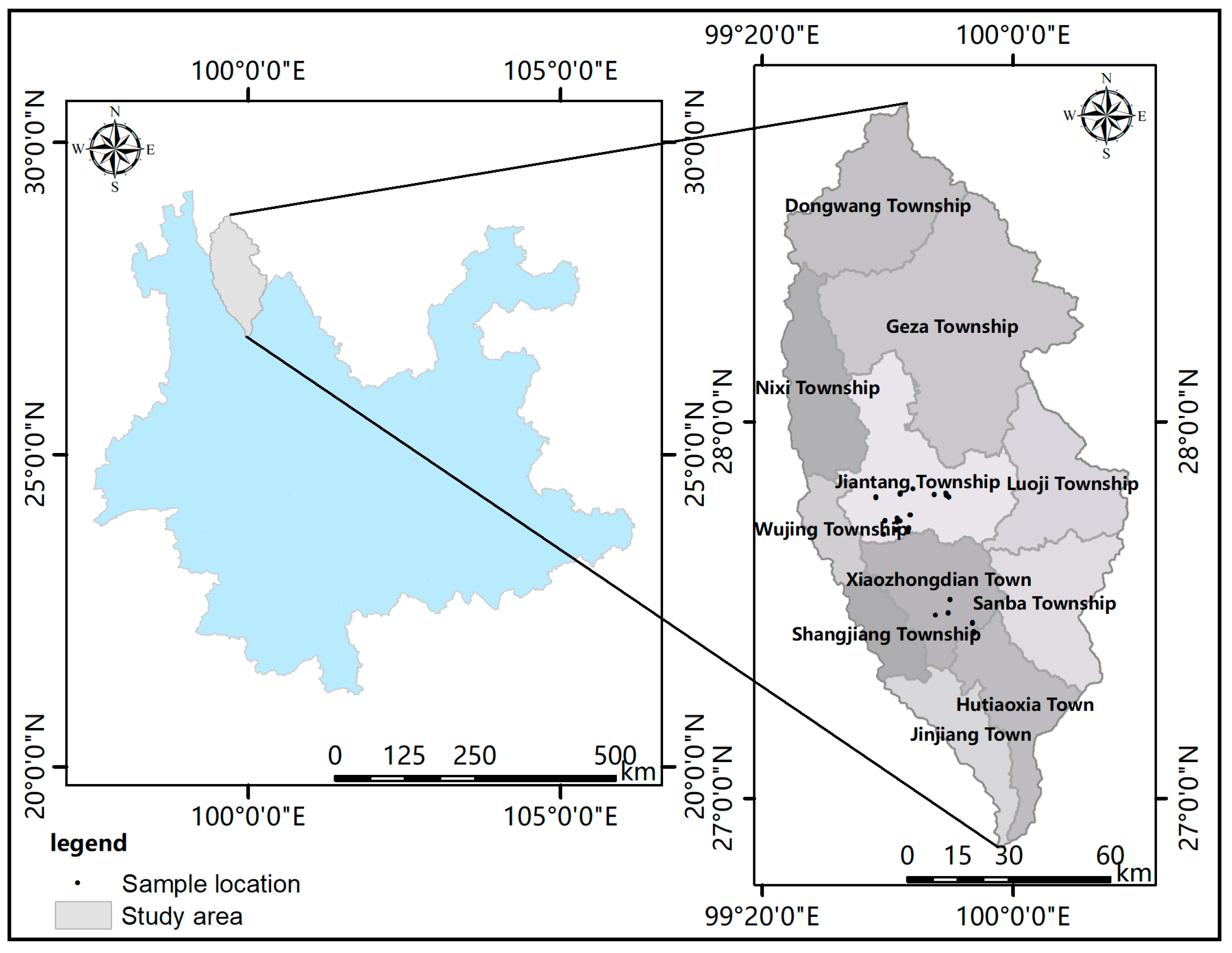
2.1. Study Area

The study was carried out in Shangri-La City, Yunnan Province, China (latitude 26°52′ N~28°52′ N, longitude 99°20′ E~100°19′ E), as shown in Figure 1. The terrain shows a high northwest and low southeast elevation. Elevation has a large altitude interval range, with an average of 3459 m. The climate is a mountainous cold-temperate monsoon climate, with four seasons that do not differ, and dry and wet seasons that are distinct. The forest coverage rate reaches 74.99%, with obvious differences in the distribution of forest vegetation from north to south. The site is predominated by Quercus semecarpifolia, Picea asperata, Abies fabri, Larix gmelinii, Pinus densata, and Pinus armandii [30,31].

2.2. ATLAS Data Products

The ICESat-2 satellite enables measurement up to 88° north and south latitudes, with a repeat cycle of 91 days. ICESat-2 carries an ATLAS instrument with a laser pulse of 10 kHz. ATLAS transmits six laser beams, and the beams are arranged along the track in three parallel groups of strong and weak beams. Each group is separated by 3.3 km. In each pair, the strong and weak beams are 2.5 km apart in the cross-track and 90 m apart along the track [32,33]. Footprints spaced 70 cm apart were produced along each track of ICESat-2 with a footprint diameter of 17 m [32,33]. ICESat-2 includes 22 standard data products of four levels. The products are named ATL01~ATL22, and the data products are stored in HDF5 format.
This study uses ATL03 (Global Geolocated Photon Data) and ATL08 (Land and Vegetation Height) as data sources. ATL03 is a secondary product that provides geospatial location information such as time, latitude, longitude, and geolocated ellipsoidal height for each photon. ATL08 is a level 3A product that is generated by estimating topography and canopy height from the ATL03 photon cloud using the ATL08 algorithm. After the photon point cloud data are denoised using the differential, regressive, and Gaussian adaptive nearest neighbor (DRAGANN) [32] algorithm, each photon is classified into noise, ground, canopy, or top of canopy photon using a photon classification algorithm. The ATL08 data product provides index ID values for each tagged photon (ground, canopy, top of canopy) that can be linked to the ATL03 data product [34]. ATL08 provides index parameters such as surface reflectance and elevation maxima, minima, means, and medians of photons per 100 m that are related to canopy and topography [32,35].
To ensure that the ATLAS orbits covered the entire study area evenly, we selected ATL08 data from January 2020 to June 2021. The data can be downloaded from the National Snow and Ice Data Center’s ICESat-2 website (https://nsidc.org/data/icesat-2, accessed on 13 January 2022).

2.3. Sample Plots Design

In order to avoid the rainy and snowy seasons in the study area, the field sample data were surveyed in November 2021. Based on the principle of representativeness, 54 circular sample plots (8.5 m radius) were set up with an area of about 0.023 hm2. The diameter and center point coordinates of the sample plots were consistent with the footprints emitted by ICESat-2/ATLAS. The survey was carried out by using the instrument of Thousand Seeker SR3 (Pro version), and the instrument was ensured to be in a fixed solution state during the sample plot centroid coordinates acquisition. The coordinates were averaged after five acquisitions. The error between the center point coordinates of all sample sites and those of the footprints was less than 0.02 m. Finally, the coordinates of sample sites, tree species, diameter at breast height, and tree height were recorded.
This study used the literature empirical method to calculate AGB (see Table 1 for details). For some difficult-to-collect tree species biomass calculation formulae, the study used the formulae of tree species with higher affinity or that of the same tree species distributed in other regions instead [36,37,38]. D and H in the footprints were substituted into the biomass formula of the corresponding tree species to calculate the AGB. Table 2 shows the statistical information of biomass in the sample site.

2.4. Determine the Scope of Woodland

In the annual basic work of Chinese forestry, regular forest land change turnover surveys are of great significance for the scientific management and development planning of forest resources. In this study, the forest land extent is determined based on the forest land change data of forest resources in 2021 (Figure 2). The data can be used to assist in the deployment of survey sample plots and for the spatial overlay analysis of footprints within the forest land extent, etc.

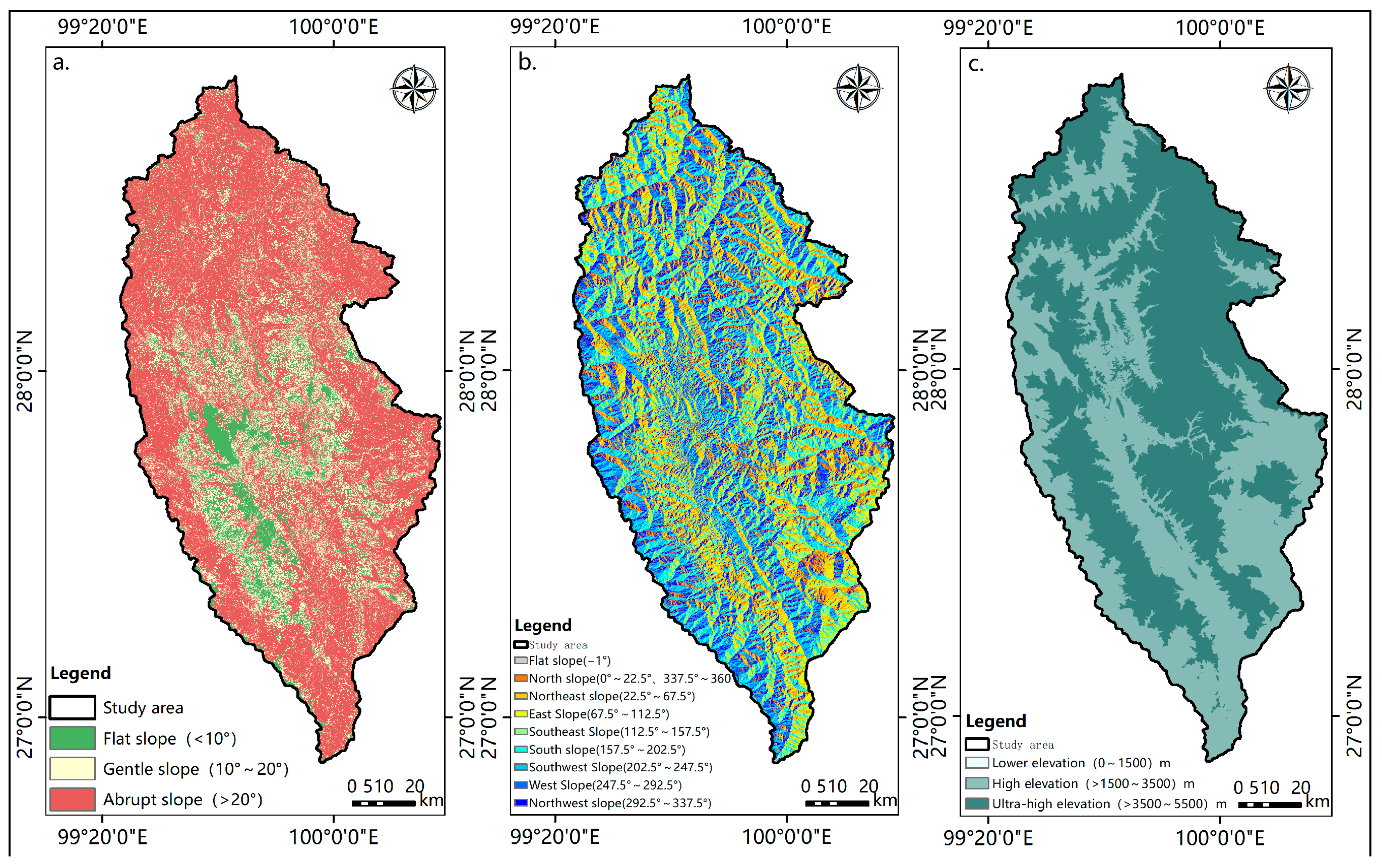
2.5. Digital Elevation Model

The Advanced Land Observing Satellite-1 (ALOS-1) was launched by Japan in 2006, and this study used the digital elevation model (DEM) with a resolution of 12.5 m acquired by the phased-array type L-band synthetic aperture radar (PALSAR) on board the satellite. The slope, aspect, and elevation of the study area were extracted using a raster surface algorithm (Figure 3).

2.6. Research Methods

The main steps for constructing AGB models based on ICESat-2/ATLAS data and performing regional-scale extrapolation of footprints AGB are as follows: photon point cloud denoising, photon point cloud classification, footprints AGB estimation model construction and evaluation, and AGB spatial interpolation and validation (as shown in Figure 4).

2.6.1. ICESat-2/ATLAS Data Processing Methods

(1)
Photon point cloud denoising algorithmA comprehensive denoising algorithm consisting of the density difference-based spatial clustering noise algorithm (DDBSCAN) [39] and the K-nearest-neighbor-based denoising algorithm (KNNB) [40] was used to remove noisy photons. Zhang et al. [41] used the maximum density difference in the DDBSCAN algorithm as the final metric in the DDBSCAN algorithm in order to compensate for the effect of photon density inconsistency on the performance of the localized statistics-based algorithm.
(2)
Photon classification algorithm
The progressive triangular irregular network (TIN) densification (PTD) method was used to distinguish the photon point cloud data into ground photons and canopy photons. Since the farthest point from the initial TIN in ICESat-2 data may be the ground point or the canopy point, this study chose the lowest elevation point below the farthest point from the initial TIN as the ground point [42].
The ICESat-2/ATLAS parameter extraction module was built based on the Python 3.7 environment with the Pycharm platform for parameter extraction. Then, the spatial overlay analysis of forest land change data of forest resources and ICESat-2 footprints was performed under ArcGIS 10.5 software. The final number of effective footprints within the forested area was determined to be 74,873 and 19,213 within the nonforested area (as shown in Figure 5).

2.6.2. Optimized RF Algorithm

Random forest (RF) is a machine learning algorithm based on statistical theory. The algorithm can quickly process a large number of datasets, and it can be directly used to train data with high-dimensional features, with strong model generalization and good fitting [43]. The parameters of machine learning algorithms are classified into two types: model parameters and model hyperparameters [44]. The hyperparameters of the RF model were optimized with the RandomizedSearchCV function [45] from the Scikit-learn library of the Python language, which was validated by the ten-fold cross-validation method. The parameters for hyperparameter optimization are n_estimators, min_samples_split, min_samples_leaf, max_features, max_depth, and bootstrap (see Table 3 for the definition of each parameter).

2.6.3. Geostatistical Methods

Geostatistics is a method for the study of natural phenomena that show a random and structural distribution in space with the help of variational functions [24]. One of the main elements of geostatistics is the kriging method. The kriging method is based on statistical correlations and spatial relationships of variables. It provides linear unbiased and optimal estimates of the values of regionalized variables within a limited area [24,29].
(1)
Semivariance function
If the regionalized variable footprints AGB Z(x) satisfies the second-order smooth or intrinsic hypothesis, the AGB variance function is as follows [25]:
r h = 1 2 N h i = 1 N h Z x i Z x i + h 2
where r h is the AGB variation function; N h is the number of pairs of points with distance equal to h in a certain direction; Z x i is the measured value of AGB of the variable at point x i ; Z x i + h is the value of AGB of the variable at point x i deviated from h.
(2)
Cokriging (COK) is a linear unbiased optimal estimation method that uses readily available variables in conjunction with hard-to-obtain variables. The formula is as follows:
Z x 0 = i = 1 n λ a i Z a x i + j = 1 m λ b j Z x j
where Z x 0 is the estimated AGB at the point to be estimated; λ a i , λ b j are the weights of the measured values of the primary variable Z 1 and the secondary variable Z 2 ; m is the number of measured values of the secondary variable Z 2 .
This study used the collaborative kriging method in the Geostatistical Analyst module of ArcGIS 10.5 software to spatially interpolate the AGB in the study area. To verify the accuracy of the cokriging interpolation results, 50,923 footprints were selected as training samples and 12,731 footprints were randomly selected as validation samples in a ratio of 8:2 from 63,654 footprints after removing the outliers. Cokriging was performed with the footprint AGB in the training sample as the main variable, and the slope factor that correlated with the AGB that covered the area of unsampled points in the sample as the covariate. Variance functions of footprint AGB and the covariate and cross-variance functions of both were fitted in GS+9.0 software, and then the footprint AGB was spatially interpolated. The interpolated AGB result was extracted by masking the study area with the forest land extent, and a map of AGB was obtained. To verify the accuracy of the interpolated AGB, we used SPSS software to establish a linear regression model, by comparing with the randomly selected validation points.

2.7. Evaluation of Model Accuracy

Leave-one-out cross-validation (LOOCV) has the advantages of low generalization error and the ability to exclude the influence of random factors, compared to other cross-validation methods. The method is suitable for a small number of samples, and the validation results are stable, reproducible, and closest to the true sample [47]. The basic principle of the leave-one-out cross-validation method is that, based on m samples, one sample is taken as the validation sample at a time, and the remaining m − 1 samples are the training samples, cycling until each sample is taken as a validation sample once. Finally, all results are averaged as an estimate of the generalization error [48]. We evaluated the model using root mean square error (RMSE), coefficient of determination (R2), and population estimation accuracy (P1) as model evaluation metrics. Each indicator was calculated as follows:
R M S E = i = 1 n y i y ^ i 2 n 1
R 2 = 1 i = 1 n y i y ^ i 2 i = 1 n y i y ¯ 2
P 1 = 1 RMSE y ¯ × 100 %
where y i is the true value; y ^ i is the estimated value; y ¯ is the mean of true value; and n is the number.
The prediction accuracy of cokriging was evaluated with the cross-validation results in the Geostatistical Analyst module [49]. The variance function model was evaluated by the coefficient of determination (R2) and the residual sum of squares (RSS), and the structure ratio (SR) was used as an indicator to evaluate the spatial correlation of the system variables. The formula is as follows:
SR = C 1 C 0 + C 1
where SR is the structure ratio; C 0 is nugget; C 1 is partial sill; C 0 + C 1 is sill.
RSS = i = 1 n y i y ^ i 2
where y i is the true value (m); y ^ i is the estimated value (m); and n is the number.

3. Results

3.1. Correlation Analysis of Model Variables

The ICESat-2/ATLAS parameters with significant correlation were screened as independent variables of the RF regression model. The SPSS 21.0 software was used to analyze the correlation between AGB and 53 variable parameters (including three topographic factors: aspect, slope, and elevation) of the sample sites by Pearson correlation coefficient analysis. Five variables were correlated with AGB at the 0.05 level, namely, Landsat percentage canopy, canopy photon rate, slope, number of photons, and apparent surface reflectance. One variable correlated with AGB at the 0.01 level was number canopy photons (see Table 4 for description of each parameter). The absolute magnitudes of the correlation coefficients of the six variables that were correlated with AGB were in the following order: number canopy photons > Landsat percentage canopy > canopy photon rate > slope > number of photons > apparent surface reflectance. The correlation analysis is shown in Figure 6.

3.2. AGB Model Construction Based on Optimized RF

To further improve the accuracy and operational efficiency of the RF model, this study performed hyperparameter optimization of the model with the help of the RandomizedSearchCV function in the Scikit-learn library [50]. In this study, 100, 1000, 3000, and 5000 sets of parameter combinations were experimented with, and 10-fold cross-validation method was used to determine the optimal parameters among 50,000 sets of parameter combinations as follows: ‘n_estimators’: 1340, ‘min_samples_split’: 2, ‘min_samples_leaf’: 2, ‘max_features’: auto, ‘max_depth’: none, ‘bootstrap’: false (see Table 3 for parameter definitions). The accuracy of the optimized model was R2 = 0.93, RMSE = 10.13 t/hm2, and P1 = 83.3% (as shown in Figure 7). The accuracy of the model was good and could be used to estimate the AGB of footprints within the woodland area of the study area.

3.3. AGB Estimation Results within ATLAS Footprints

The AGB of footprints was estimated using an optimized RF algorithm, and the AGB of 74,873 footprints was obtained in the study area. The population AGB of footprints was 1.32 × 10⁵ t with the mean of 77.41 t/hm2, the maximum of 126 t/hm2, and the minimum of 0.88 t/hm2. The spatial distribution of AGB of footprints was plotted according to the coordinates of the center of footprints in the study area (as shown in Figure 8a). Figure 8a demonstrates that the population AGB of footprints is relatively large in the study area, but the AGB shows uneven distribution and large regional differences. The main reason is that Shangri-La is located at low latitudes and high altitudes, which means it is susceptible to the influence of vertical zonation and forms a unique “vertical climate”. The distribution of large AGB footprints was from the north to the southeast and it was mainly concentrated in the northern region, which coincided with the spatial distribution of forest stock in the study area (as shown in Figure 8b). The areas with large AGB were mostly natural scenic areas, while the areas with small AGB were mainly distributed in snow- and ice-covered areas, next to water areas, and next to cities, which also verified the validity of the results of the footprints AGB estimation model.

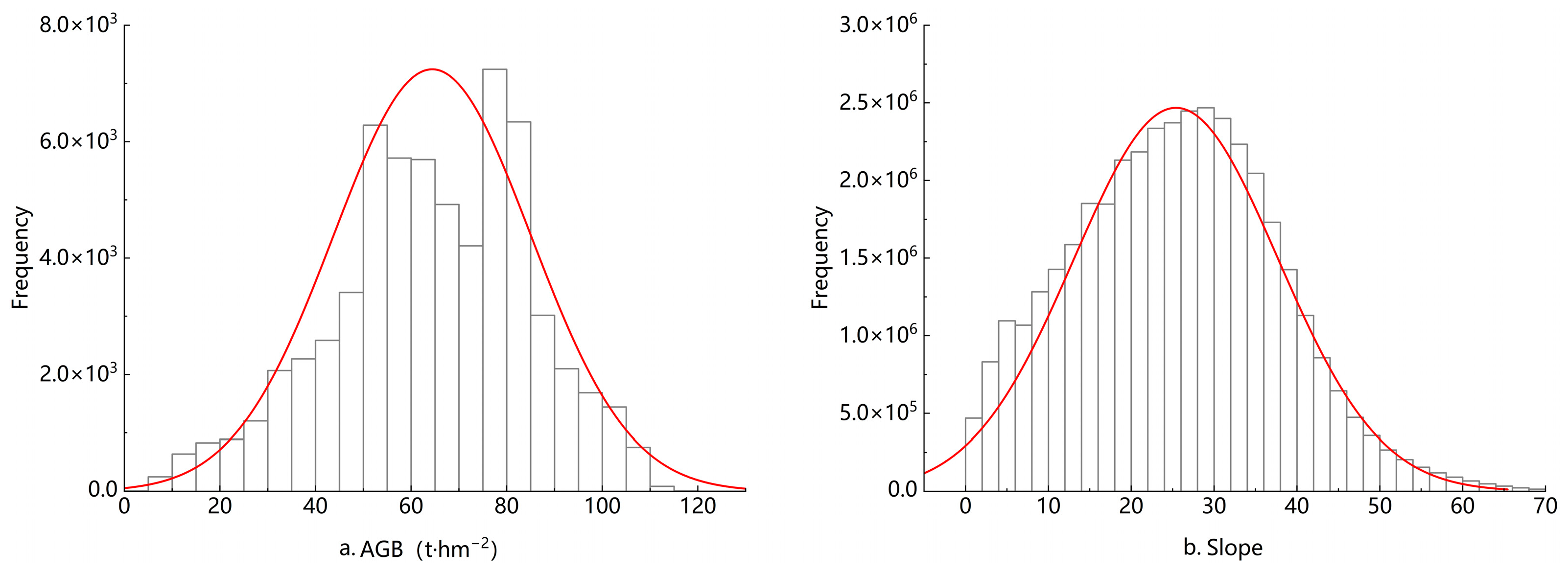
3.4. Statistical Analysis of Interpolated Variables and Determination of Variance Functions

According to the results of the correlation analysis in Section 3.1, the slope factor, which was easily obtained and significantly correlated with AGB, was selected as the covariable of the cokriging method, and we analyzed the distribution characteristics of the samples after removing the outliers. From Figure 9, it is clear that the AGB and slope factor obeyed normal distribution and satisfied the interpolation conditions of cokriging (see Table 5 for statistical information).
The interpolation results of different variance functions are different, and in order to determine the optimal variance function model, the variance function needs to be simulated before interpolation is performed. In this study, three models (spherical, exponential, and Gaussian) were selected to fit the variance functions under GS+9.0 software. The results of fitting each model are shown in Table 6. The R2 of all three models were similar, and the RSS of the spherical and Gaussian models were the smallest; both were 2.65 × 10⁻⁴. The nugget is often used to measure the variability of variables and experimental error at small sampling scales [29]. Because the nugget of the spherical model was 0.01, which was the smallest degree of variation, we finally selected the spherical model as the optimal variance function model for the collaborative kriging method.
The SR is used to measure the degree of spatial autocorrelation of the system variables. SR > 75%, SR between 25% and 75%, and SR < 25%, respectively, indicate strong, moderate, and weak spatial autocorrelation of the variables [51]. The SR of the main variable of the spherical model was 94% in Table 6, which was much greater than 75%. This indicated that the AGB had a strong spatial correlation in the study area. The main reason is that biomass distribution is influenced by spatial factors such as topographic factors, climate, and soil type. The variance function of ABG was fitted with nugget of 0.01, sill of 0.22, and range of 6700.00 m. The spatial variability reaches its maximum when the range is exceeded and there is no correlation between two points. The spherical model equation for AGB was as follows:
γ h = 0 , h = 0 0.01 + 0.21 3 h 13 , 400 h 3 6.02 × 10 11 , 0 < h 6700 0.22 , h > 6700
The covariate slope variation function was fitted with nugget of 0.10, sill of 125.90, and range of 8300.00 m. The spherical model equation for the covariate slope was as follows:
h = 0 , h = 0 0.10 + 125.89 3 h 16 , 600 h 3 1.14 × 10 12 , 0 < h 8300 125.90 , h > 8300
A cross-variance function was established based on the spatial correlation between AGB and slope, with nugget of 0.25, sill of 1.42, and range of 7200.00 m. The Gaussian model equation was as follows:
γ h = 0 , h = 0 0.25 + 1.16 3 h 14 , 400 h 3 7.47 × 10 11 , 0 < h 7200 1.42 , h > 7200

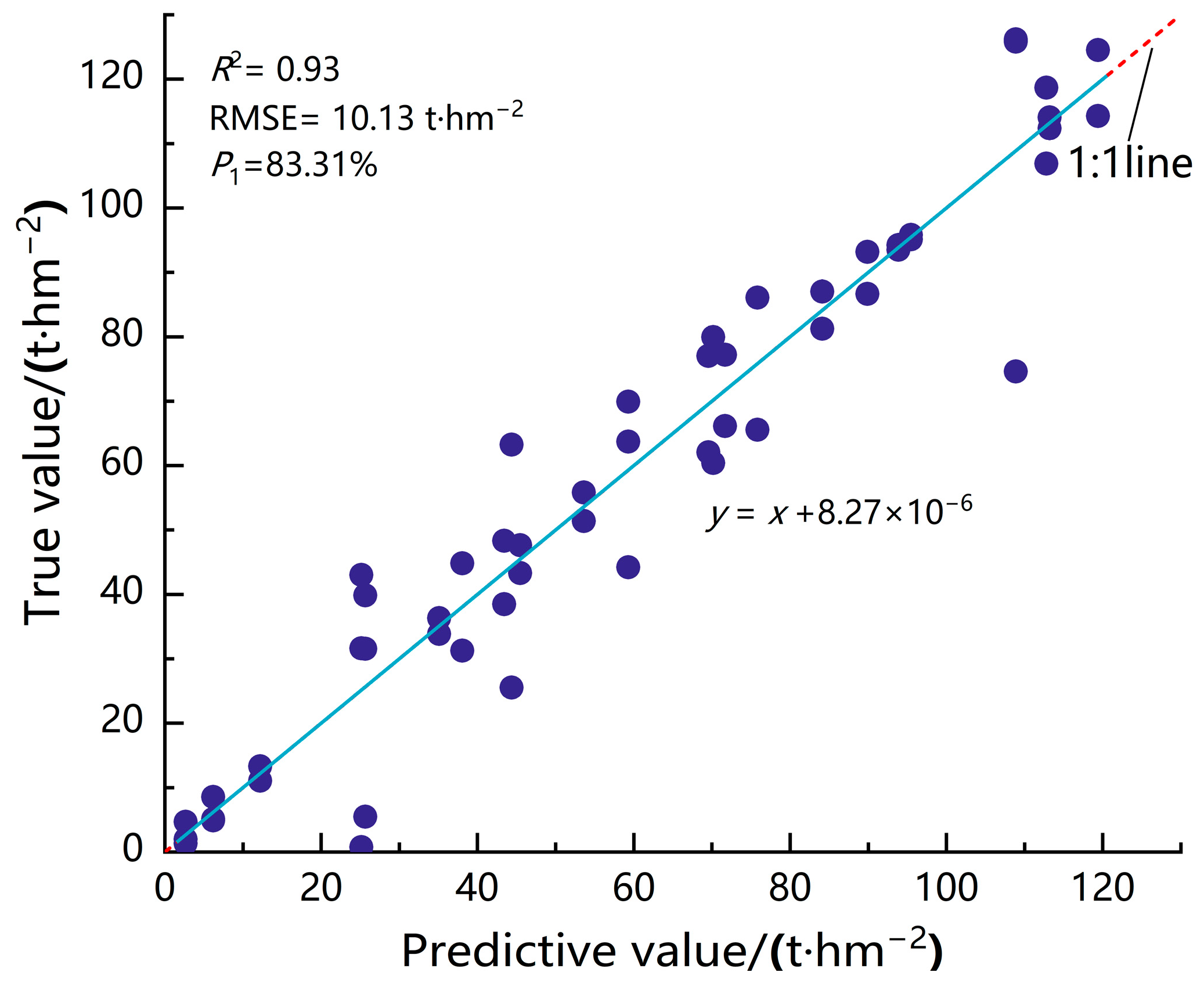
3.5. Validation of Interpolation Results

The study examined the interpolation results using 12,731 randomly selected footprints, and the results are shown in Figure 10. The linear equation was y = 0.47x + 33.62, R2 = 0.43, RMSE = 5.29 t/hm2, and the interpolation results showed a certain convergence trend with the AGB of the footprints.

3.6. Spatial Distribution Analysis of AGB

Figure 11 reveals the spatial distribution and standard error prediction results of AGB generated by collaborative kriging in Shangri-La. The population AGB was 6.07 × 10⁷ t. As shown in Figure 11a, the spatial distribution of AGB was heterogeneous, and the SR of the variables was 94.0% (Table 6), indicating that spatial correlation was one of the factors that led to the heterogeneous spatial distribution of AGB in the study area. On the other hand, this is related to the complex topographic structure and the typical “vertical climate” of Shangri-La. The result was consistent with the spatial distribution of forest stock in the study area in 2021 shown in Figure 8. In addition, Figure 11b,c display smaller standard error of prediction in the area of ICESat-2 footprints distribution, demonstrating that the large sampling density of ATLAS data can improve spatial interpolation accuracy.

4. Discussion

4.1. Validity Analysis of Estimation Results

The estimation of AGB was performed using traditional-class Forest Resources Planning and Design Survey and remote sensing techniques in Shangri-La. Feng et al. [31] used texture factors extracted from ZY3-01 data as independent variables and footprints AGB predicted from GLAS data as dependent variables to establish a multiple stepwise regression model to estimate that the population AGB was 1.3 × 10⁸ t in Shangri-La. Yue [52] used Landsat TM images as the data source and support vector machines as the optimal modeling method to establish a biomass estimation model for four dominant tree species in Shangri-La, and the population AGB of the four tree species was 1.407 × 10⁸ t. Wang et al. [53] established a remote sensing estimation model for the biomass of four constructive tree species in Shangri-La and estimated the population AGB of four tree species to be 1.14 × 10⁸ t. In 2021, the AGB was estimated to be 7.35 × 10⁷ t, which was estimated by Wang et al. [36] using data from the 2016 Forest Resources Planning and Design Survey with a biomass model for different types of dominant tree species in Shangri-La. Because the results come from the 2016 Forest Resources Planning and Design Survey, it is reliable as the reference standard for the estimation accuracy of AGB in this study. The estimation of population AGB was 6.07 × 10⁷ t in this study, which was the same order of magnitude as the reference standard, while the estimations of other scholars were quite different from the reference standard [31,52,53]. Finally, we describe the results of the absolute precision of the estimation, which was 82.6%.

4.2. Elimination of Error Transmission Feasibility Analysis

In this paper, we investigated the feasibility of ICESat-2/ATLAS data for estimating AGB in montane forests, and an optimized random forest model was used to establish a montane AGB estimation model. The results showed that despite the complex terrain, broad elevation difference, and large forest cover in the study area [30], the estimation accuracy of the RF model using ICESat-2 data was still high. The main reason might possibly be that ICESat-2/ATLAS has a larger density and smaller footprint area compared to ICESat-1/GLAS. Even if the terrain is undulating, the footprints of ATLAS are less influenced by the terrain than GLAS data, and ATLAS data are more suitable for inversion of forest measurement parameters in complex mountainous terrain. In order to further improve the accuracy of AGB scale nudging and reduce the error transfer in the nudging process, other models, for example, other machine learning methods such as K-nearest neighbors (KNN) [48] or deep learning [54], suitable for handling multidimensional data, can be selected for further examination. In addition, Bayesian optimization [55] can be tried for random forest hyperparameter tuning, which can relatively reduce the number of iterations in the optimization process and make full use of the information from each test point. Narine et al. [21] found that strong beam inversion had higher accuracy than weak beam inversion for AGB, with R2 = 0.60 for the strong beam model and R2 = 0.37 for the weak beam model. Therefore, in order to reduce error transfer, further studies should investigate the strong beam for prediction. On the other hand, Moradi et al. found that indices extracted from Sentinel-2 multispectral imagery can provide good results in the AGB estimation of the Hyrcanian Forests and a Mediterranean coppice oak forest. In this sense, future studies can use ICESat-2 in collaboration with Sentinel 2 data for multisource remote sensing synergy to estimate AGB [56,57].

4.3. Analysis of the Interpolation Result String Phenomenon Is Obvious

As described in Figure 8 and Figure 11, the spatial distribution pattern of AGB is consistent with that of forest stock in Shangri-La City. However, the strong spatial correlation between biomass and ATLAS data affected the prediction results of cokriging interpolation. Figure 11b,c show the small prediction standard error of the location of the footprints distribution, which validates the conclusion of Tsui et al. [27] that the narrower the sampling band interval, the lower the standard error of the predicted biomass. It is also consistent with the conclusion that the higher the number of samples within the same topographic cell, the higher the interpolation accuracy [58]. In the present study, the large-overlap ATLAS footprints were used as interpolation sample points, but the spatial distribution of AGB was influenced by the string effect (as shown in Figure 11). Further research is needed to optimize the number or layout of sample points for ATLAS data at different scales to improve the accuracy. In addition, since the satellite-based LiDAR footprints are generally uniformly distributed along the track on the ground, satellite-based LiDAR data from different sensor platforms can be fused to increase the randomness of the footprint distribution in the future, which can mitigate the string effect [59]. Furthermore, the choice of interpolation methods and covariates may cause the interpolation results to be affected by string effect under different topographic conditions. In this study, the cokriging interpolation could reduce the smoothing effect, but the effect was not eliminated, making the AGB estimations underestimated. Accordingly, regression kriging and sequential Gaussian co-interpolation methods [28,60] can be carried out. In addition, mainly considering that the study area was located in a mountainous region with complex topography, the slope factor was chosen as a covariate. Furthermore, other factors with strong spatial autocorrelation, such as climate factors and vegetation index, can be considered comprehensively as covariates for estimation in flatter areas.

5. Conclusions

In the present study, a hyperparameter-optimized RF model was constructed after parameter extraction for ICESat-2 footprints within the forested area using data of 54 measured sample plots. Then, we selected the spherical model to fit the variance function based on the estimations of all footprint AGB. Finally, the continuous spatial distribution of AGB was obtained by interpolation using the cokriging method. Our results demonstrated that the optimized RF model had a good effect for estimation of AGB within the footprint. The model had R2 = 0.93, RMSE = 10.13 t/hm2, and P1 = 83.3%. The spatial distribution pattern of estimated AGB is basically consistent with that of forest stock in the study area. The estimated population AGB was 6.07 × 10⁷ t in Shangri-La, with an absolute accuracy of 82.6%. The findings make full use of the advantage of easy access to ATLAS data and dense footprints, and can quickly and effectively extrapolate the biomass scale while optimizing the AGB estimation model.

Author Contributions

Conceptualization, Q.S., L.X. and H.S.; methodology, H.S.; formal analysis, H.S.; investigation, L.X., S.Q. and Z.W.; resources, Q.S.; writing—original draft preparation, H.S.; writing—review and editing, H.S., Q.S. and L.X.; software visualization, L.X.; visualization, H.S. and L.X.; supervision, Q.S.; funding acquisition, Q.S. All authors have read and agreed to the published version of the manuscript.

Funding

This research was funded by the National Natural Science Foundation of China (Nos. 31860205 and 31460194), Yunnan Provincial Education Department Scientific Research Fund Project (No. 2021Y249), China, in 2021.

Data Availability Statement

Not applicable.

Acknowledgments

The authors would like to thank the NASA NSIDC for distributing the ICESat-2 data (https://search.earthdata.nasa.gov, accessed on 13 January 2022), and the anonymous reviewers and members of the editorial team for their constructive comments.

Conflicts of Interest

The authors declare no conflict of interest.

References

  1. Meng, L. Distribution of Forest Biomass for Main Forest Types in the Forestry Administration of Daxinganling Based on Geostatistics. Master’s Thesis, Northeast Forestry University, Heilongjiang, China, 2017. (In Chinese). [Google Scholar]
  2. Tuominen, S.; Eerikäinen, K.; Schibalski, A.; Haakana, M.; Lehtonen, A. Mapping biomass variables with a multi-source forest inventory technique. Silva Fenn. 2010, 44, 109–119. [Google Scholar] [CrossRef] [Green Version]
  3. Kangas, A.; Maltamo, M. Forest Inventory: Methodology and Applications; Springer Science & Business Media: Cham, Switzerland, 2006; Volume 10. [Google Scholar] [CrossRef]
  4. López-Serrano, P.M.; López Sánchez, C.A.; Solís-Moreno, R.; Corral-Rivas, J.J. Geospatial estimation of above ground forest biomass in the Sierra Madre Occidental in the state of Durango, Mexico. Forests 2016, 7, 70. [Google Scholar] [CrossRef] [Green Version]
  5. Peduzzi, A.; Wynne, R.H.; Fox, T.R.; Nelson, R.F.; Thomas, V.A. Estimating leaf area index in intensively managed pine plantations using airborne laser scanner data. For. Ecol. Manag. 2012, 270, 54–65. [Google Scholar] [CrossRef] [Green Version]
  6. Atwood, D.K.; Andersen, H.E.; Matthiss, B.; Holecz, F. Impact of Topographic Correction on Estimation of Aboveground Boreal Biomass Using Multi-temporal, L-Band Backscatter. IEEE J. Sel. Top. Appl. Earth Obs. Remote Sens. 2014, 7, 3262–3273. [Google Scholar] [CrossRef]
  7. Vatandaşlar, C.; Abdikan, S. Carbon stock estimation by dual-polarized synthetic aperture radar (SAR) and forest inventory data in a Mediterranean forest landscape. J. For. Res. 2021, 33, 827–838. [Google Scholar] [CrossRef]
  8. Disney, M. Terrestrial LiDAR: A 3D revolution in how we look at trees. New Phytol. 2018, 222, 15517. [Google Scholar] [CrossRef] [Green Version]
  9. Pitkänen, T.P.; Raumonen, P.; Kangas, A. Measuring stem diameters with TLS in boreal forests by complementary fitting procedure. ISPRS J. Photogramm. Remote Sens. 2019, 147, 294–306. [Google Scholar] [CrossRef]
  10. Wang, Y.; Ni, W.; Sun, G.; Chi, H.; Zhang, Z.; Guo, Z. Slope-adaptive waveform metrics of large footprint lidar for estimation of forest aboveground biomass. Remote Sens. Environ. 2019, 224, 386–400. [Google Scholar] [CrossRef]
  11. Lefsky, M.A.; Harding, D.J.; Keller, M.; Cohen, W.B.; Carabajal, C.C.; Del Bom Espirito-Santo, F.; Hunter, M.O.; de Oliveira, R., Jr. Estimates of forest canopy height and aboveground biomass using ICESat. Geophys. Res. Lett. 2005, 32, L22S02. [Google Scholar] [CrossRef]
  12. Markus, T.; Neumann, T.; Martino, A.; Abdalati, W.; Brunt, K.; Csatho, B.; Farrell, S.; Fricker, H.; Gardner, A.; Harding, D. The Ice, Cloud, and land Elevation Satellite-2 (ICESat-2): Science requirements, concept, and implementation. Remote Sens. Environ. 2017, 190, 260–273. [Google Scholar] [CrossRef]
  13. Sawruk, N.; Burns, P.; Edwards, R.; Litvinovitch, V.; Hovis, F. Flight Lasers Transmitter Development for Nasa Ice Topography Icesat-2 Space Mission. In Proceedings of the IGARSS 2018—2018 IEEE International Geoscience and Remote Sensing Symposium, Valencia, Spain, 22–27 July 2018. [Google Scholar] [CrossRef]
  14. Hu, Y.; Wu, F.; Sun, Z.; Lister, A.; Gao, X.; Li, W.; Peng, D. The Laser Vegetation Detecting Sensor: A Full Waveform, Large-Footprint, Airborne Laser Altimeter for Monitoring Forest Resources. Sensors 2019, 19, 1699. [Google Scholar] [CrossRef] [Green Version]
  15. Moussavi, M.S.; Abdalati, W.; Scambos, T.; Neuenschwander, A. Applicability of an automatic surface detection approach to micro-pulse photon-counting lidar altimetry data: Implications for canopy height retrieval from future ICESat-2 data. Int. J. Remote Sens. 2014, 35, 5263–5279. [Google Scholar] [CrossRef]
  16. Brown, M.; Escobar, V. NASA’s Early Adopter Program Links Satellite Data to Decision Making. Remote Sens. 2019, 11, 406. [Google Scholar] [CrossRef] [Green Version]
  17. Wulder, M.A.; Bater, C.W.; Coops, N.C.; Hilker, T.; White, J.C. The role of LiDAR in sustainable forest management. For. Chron. 2008, 84, 807–826. [Google Scholar] [CrossRef] [Green Version]
  18. Yue, C.; Zhen, Y.; Xing, Y.; Pang, Y.; Li, S.; Cai, L.; He, H. Technical and application development study of space-borne LiDAR in forestry remote sensing. Infrared Laser Eng. 2020, 49, 105–114. [Google Scholar] [CrossRef]
  19. Narine, L.L.; Popescu, S.; Neuenschwander, A.; Zhou, T.; Srinivasan, S.; Harbeck, K. Estimating aboveground biomass and forest canopy cover with simulated ICESat-2 data. Remote Sens. Environ. 2019, 224, 37. [Google Scholar] [CrossRef]
  20. Narine, L.L.; Popescu, S.C.; Malambo, L. Synergy of ICESat-2 and Landsat for mapping forest aboveground biomass with deep learning. Remote Sens. 2019, 11, 1503. [Google Scholar] [CrossRef]
  21. Narine, L.L.; Popescu, S.C.; Malambo, L. Using ICESat-2 to estimate and map forest aboveground biomass: A first example. Remote Sens. 2020, 12, 1824. [Google Scholar] [CrossRef]
  22. Li, W.; Niu, Z.; Shang, R.; Qin, Y.; Wang, L.; Chen, H. High-resolution mapping of forest canopy height using machine learning by coupling ICESat-2 LiDAR with Sentinel-1, Sentinel-2 and Landsat-8 data. Int. J. Appl. Earth Obs. Geoinf. 2020, 92, 102163. [Google Scholar] [CrossRef]
  23. Silva, C.A.; Duncanson, L.; Hancock, S.; Neuenschwander, A.; Thomas, N.; Hofton, M.; Fatoyinbo, L.; Simard, M.; Marshak, C.Z.; Armston, J. Fusing simulated GEDI, ICESat-2 and NISAR data for regional aboveground biomass mapping. Remote Sens. Environ. 2021, 253, 112234. [Google Scholar] [CrossRef]
  24. Feng, Y. Spatial Statistics Theory and Its Application in Forestry; Chinese Forestry Publishing House: Beijing, China, 2008. (In Chinese) [Google Scholar]
  25. Wang, H.; Peng, D.; FAn, Y.; Li, W.; Zhang, C. Spatial Modeling of Forest Stock Volume Based onAuxiliary In-formation. Trans. Chin. Soc. Agric. Mach. 2016, 47, 7. (In Chinese) [Google Scholar]
  26. Hajj, M.E.; Baghdadi, N.; Fayad, I.; Vieilledent, G.; Bailly, J.-S.; Minh, D.H.T. Interest of integrating spaceborne LiDAR data to improve the estimation of biomass in high biomass forested areas. Remote Sens. 2017, 9, 213. [Google Scholar] [CrossRef] [Green Version]
  27. Tsui, O.W.; Coops, N.C.; Wulder, M.A.; Marshall, P.L. Integrating airborne LiDAR and space-borne radar via multivariate kriging to estimate above-ground biomass. Remote Sens. Environ. 2013, 139, 340–352. [Google Scholar] [CrossRef]
  28. Jin, Y.; Zhang, M.; Guo, H.; He, W. Comparison of Forest Carbon Spatial Distribution Based on Kriging In-terpolation and Sequential Gaussian Co-Simulation. J. Southwest For. Univ. 2013, 33, 32–37, 45. (In Chinese) [Google Scholar]
  29. He, P.; Zhang, H.; Lei, X.; Xu, G.; Gao, X. Estimation of forest Above-Ground Biomass based on geostatistics. Sci-Entia Silvae Sin. 2013, 49, 101–109. (In Chinese) [Google Scholar]
  30. Xu, D.; Zhang, J.; Bao, R.; Liao, Y.; Han, D.; Liu, Q.; Cheng, T. Temporal and Spatial Variation of Aboveground Biomass of Pinus densata and Its Drivers in Shangri-La, CHINA. Int. J. Environ. Res. Public Health 2022, 19, 400. [Google Scholar] [CrossRef]
  31. Feng, W.; Wang, L.; Xie, J.; Yue, C.; Zheng, Y.; Yu, L. Estimation of Forest Biomass Based on Muliti-Source Remote Sensing Data Set-a Case Study of Shangri-La County. ISPRS Ann. Photogramm. Remote Sens. Spat. Inf. Sci. 2018, IV-3, 77–81. [Google Scholar] [CrossRef] [Green Version]
  32. Neuenschwander, A.; Pitts, K. The ATL08 land and vegetation product for the ICESat-2 Mission. Remote Sens. Environ. 2019, 221, 247–259. [Google Scholar] [CrossRef]
  33. Brown, M.E.; Arias, S.D.; Neumann, T.; Jasinski, M.F.; Posey, P.; Babonis, G.; Glenn, N.F.; Birkett, C.M.; Escobar, V.M.; Markus, T. Applications for ICESat-2 Data: From NASA’s Early Adopter Program. IEEE Geosci. Remote Sens. Mag. 2016, 4, 24–37. [Google Scholar] [CrossRef]
  34. Neuenschwander, A.L.; Magruder, L.A. Canopy and Terrain Height Retrievals with ICESat-2: A First Look. Remote Sens. 2019, 11, 1721. [Google Scholar] [CrossRef] [Green Version]
  35. Neumann, T.; Brenner, A.; Hancock, D.; Robbins, J.; Saba, J.; Harbeck, K.; Gibbons, A. Ice, Cloud, and Land Elevation Satellite–2 (Icesat-2) Project: Algorithm Theoretical Basis Document (ATBD) for Global Geolocated Photons (ATL03); Goddard Space Flight Center: Greenbelt, MD, USA, 2019.
  36. Wang, J.; Tang, W. Estimation and analysis of aboveground biomass and carbon storage of arbor forest based on forest resource planning and design survey data: A case study of Shangri-La City. J. Green Sci. Technol. 2021, 23, 14–16. (In Chinese) [Google Scholar]
  37. Yuan, L. Natural forest biomass of Pinus armandii plantation in Yunlong Tianchi Nature Reserve of Yunnan Province. Prot. For. Sci. Technol. 2018, 38, 13–15. (In Chinese) [Google Scholar]
  38. Zeng, W.; Sun, X.; Wang, L.; Wang, W.; Pu, Y. Developing stand volume, biomass and carbon stock models for ten major forest types in forest region of northeastern China. J. Beijing For. Univ. 2021, 43, 1–8. (In Chinese) [Google Scholar]
  39. Zhang, J.; Kerekes, J. An adaptive density-based model for extracting surface returns from photon-counting laser altimeter data. IEEE Geosci. Remote Sens. Lett. 2014, 12, 726–730. [Google Scholar] [CrossRef]
  40. Xia, S.B.; Wang, C.; Xi, X.H.; Luo, S.Z.; Zeng, H.C. Point cloud filtering and tree height estimation using airborne experiment data of ICESat-2. J. Remote Sens 2014, 18, 1199–1207. [Google Scholar]
  41. Zhang, J.; Tian, J.; Li, X.; Wang, L.; Chen, B.; Gong, H.; Ni, R.; Zhou, B.; Yang, C. Leaf area index retrieval with ICESat-2 photon counting LiDAR. Int. J. Appl. Earth Obs. Geoinf. 2021, 103, 102488. [Google Scholar] [CrossRef]
  42. Nie, S.; Wang, C.; Dong, P.; Xi, X.; Luo, S.; Qin, H. A revised progressive TIN densification for filtering airborne LiDAR data. Measurement 2017, 104, 70–77. [Google Scholar] [CrossRef]
  43. Breiman, L.; Breiman, L.; Cutler, R.A. Random Forests Machine Learning. J. Clin. Microbiol. 2001, 2, 199–228. [Google Scholar]
  44. Luo, G. A review of automatic selection methods for machine learning algorithms and hyper-parameter values. Netw. Model. Anal. Health Inform. Bioinform. 2016, 5, 18. [Google Scholar] [CrossRef]
  45. Bergstra, J.; Bengio, Y. Random search for hyper-parameter optimization. J. Mach. Learn. Res. 2012, 13, 281–305. [Google Scholar]
  46. Geurts, P.; Ernst, D.; Wehenkel, L. Extremely randomized trees. Mach. Learn. 2006, 63, 3–42. [Google Scholar] [CrossRef] [Green Version]
  47. Yu, H.; Ni, J.; Xu, S. Pre-evaluation strategy of harmfulness caused by class imbalance based on Leave-one-out Cross Validation. J. Chin. Comput. Syst. 2012, 33, 2287–2292. (In Chinese) [Google Scholar]
  48. Xie, F.; Shu, Q. Estimation and Mapping of Forest Aboveground Biomass Based on k-NN Model and Remote Sensing. Master’s Thesis, Southwest Forestry University, Kunming, China, 2019. (In Chinese). [Google Scholar]
  49. Zhen, X.; Lu, L. Geostatistics (Modern Spatial Statistics); Science Press: Beijing, China, 2018. (In Chinese) [Google Scholar]
  50. Song, H.; Shu, Q.; Xi, L.; Qiu, S.; Wei, Z.; Yang, Z. Remote sensing estimation of forest above-ground biomass based on spaceborne lidar ICESat-2/ATLAS data. Trans. Chin. Soc. Agric. Eng. 2022, 38, 191–199. (In Chinese) [Google Scholar]
  51. SUn, L.; Chang, Q.; Zhao, Y.; Zhang, Y. Spatial distribution of soil nutrients in hilly region of Southern Shaanxi. J. Northwest AF Univ. 2015, 43, 162–168, 174. (In Chinese) [Google Scholar]
  52. Yue, C. Forest Biomass Estimation in Shangri-La County based on Remote Sensing. Ph.D. Thesis, Beijing Forestry University, Beijing, China, 2012. (In Chinese). [Google Scholar]
  53. Wang, J.; Chen, P.; Xu, S.; Wang, X.; Chen, F. Forest Biomass Estimation in Shangri-La based on the Remote Sensing. J. Zhejiang A F Univ. 2013, 30, 325–329. (In Chinese) [Google Scholar]
  54. Hatcher, W.G.; Yu, W. A survey of deep learning: Platforms, applications and emerging research trends. IEEE Access 2018, 6, 24411–24432. [Google Scholar] [CrossRef]
  55. Victoria, A.H.; Maragatham, G. Automatic tuning of hyperparameters using Bayesian optimization. Evol. Syst. 2021, 12, 217–223. [Google Scholar] [CrossRef]
  56. Moradi, F.; Sadeghi, S.M.M.; Heidarlou, H.B.; Deljouei, A.; Boshkar, E.; Borz, S.A. Above-ground biomass estimation in a Mediterranean sparse coppice oak forest using Sentinel-2 data. Ann. For. Res. 2022, 65, 165–182. [Google Scholar] [CrossRef]
  57. Moradi, F.; Darvishsefat, A.A.; Pourrahmati, M.R.; Deljouei, A.; Borz, S.A. Estimating Aboveground Biomass in Dense Hyrcanian Forests by the Use of Sentinel-2 Data. Forests 2022, 13, 104. [Google Scholar] [CrossRef]
  58. Zhang, J.; Fu, W.; Du, Q.; Zhang, G.; Jiang, P. Effects of topographical condition and sampling number on the interpolation precision of forest litter carbon density. Chin. J. Appl. Ecol. 2013, 24, 2241–2247. (In Chinese) [Google Scholar]
  59. Liu, X.; Su, Y.; Hu, T.; Yang, Q.; Liu, B.; Deng, Y.; Tang, H.; Tang, Z.; Fang, J.; Guo, Q. Neural network guided interpolation for mapping canopy height of China’s forests by integrating GEDI and ICESat-2 data. Remote Sens. Environ. 2022, 269, 112844. [Google Scholar] [CrossRef]
  60. Liu, L.; Wang, H.; Dai, W.; Yang, X.; Li, X. Spatial heterogeneity of soil organic carbon and nutrients in low mountain area of Changbai Mountains. Chin. J. Appl. Ecol. 2014, 25, 2460–2468. (In Chinese) [Google Scholar]
Figure 1. Location of the study area and the sample circles.
Forests 14 00013 g001
Figure 2. Statistics forest land change data in 2021.
Forests 14 00013 g002
Figure 3. Slope, aspect, and elevation maps of the study area. (a) Slope; (b) aspect; (c) elevation.
Forests 14 00013 g003
Figure 4. Technology roadmap.
Forests 14 00013 g004
Figure 5. Schematic diagram of effective footprints in the study area. (a) Forest footprints. (b) Nonforest footprints.
Forests 14 00013 g005
Figure 6. Correlation between 6 parameters and footprint AGB.
Forests 14 00013 g006
Figure 7. Optimized random forest AGB model-fitting accuracy map.
Forests 14 00013 g007
Figure 8. Spatial distribution of AGB of ICESat-2 footprints and forest stock in 2021. (a) Footprints AGB. (b) Forest stock in 2021.
Forests 14 00013 g008
Figure 9. Variable distribution map. (a) AGB. (b) Slope.
Forests 14 00013 g009
Figure 10. Interpolation accuracy validation scatter plots.
Forests 14 00013 g010
Figure 11. Spatial distribution of AGB in the study area. (a) Predicted results. (b) Standard error prediction. (c) Standard error of overlapping footprint prediction results.
Forests 14 00013 g011
Table 1. Biomass model of main tree species in Shangri-La City.
Tree SpeciesDiameter at Breast HeightAboveground Biomass Model
Abies fabriD ≥ 5MA = 0.06127D2.05753H0.50839 [36]
D < 5MA = 0.19406D1.34122H0.50839 [36]
QuercusD ≥ 5MA = 0.07806D2.06321H0.57393 [36]
D < 5MA = 0.22999D1.39183H0.57393 [36]
Pinus densataD > 0MA = 0.0730D2.3560H0.1090 [36]
Picea asperataD ≥ 5MA = 0.09152D2.2106H0.25663 [36]
D < 5MA = 0.16923D1.82866H0.25663 [36]
Pinus yunnanensisD > 0MA = 0.070231D2.10392H0.41120 [36]
Larix gmeliniiD ≥ 5MA = 0.05577D2.01549H0.59146 [36]
D < 5MA = 0.15678D1.37332H0.59146 [36]
Pinus armandiiD > 0MA = 0.009512(D2H)1.138665 [37]
PopulusD > 0MB = 2.83252G0.000 00 H ¯ −0.46615M [38]
M = 1.37840G1.08641 H ¯ 0.57336 [38]
MA is stand biomass (kg), MB is biomass per unit area (t/hm2), M is volume per unit area (m3/hm2), D is diameter at breast height (cm), H is tree height (m), H ¯ is stand mean height (m), and G is stand section area (m2/hm2).
Table 2. Statistical information of AGB in plots.
NumbersMeanMean Standard ErrorStandard DeviationMaxMin
5459.485.2937.45126.000.88
Note: The statistical units in the table are t·hm−2.
Table 3. Description of random forest algorithm optimization parameters.
ParametersDescription [43,46]Type
n_estimatorsThe number of trees in the forest.int
min_samples_splitThe minimum number of samples required to split an internal node.int or float
min_samples_leafThe minimum number of samples required to be at a leaf node.int or float
max_featuresThe number of features to consider when looking for the best split.int or float
max_depthThe maximum depth of the tree.int
bootstrapWhether bootstrap samples are used when building trees.bool
Table 4. Parameter definitions for significant correlation with AGB.
Serial NumberParameterLong NameDescription
1n_seg_phNumber of photonsNumber of photons within each land segment.
2asrApparent surface reflectanceApparent surface reflectance.
3landsat_percLandsat percentage canopyAverage percentage value of the valid (value ≤ 100) Landsat Tree Cover Continuous Fields product for each 100 m segment.
4n_ca_photonsNumber canopy photonsThe number of photons classified as canopy within the segment.
5photon_rate_canCanopy photon rateCalculated photon rate of canopy photons within each 100 m segment.
6SlopeSlopeCalculated based on DEM.
Table 5. Statistical characteristics of AGB and covariable.
VariablesMeanStandard DeviationMaxMin
AGB/(t·hm−2)64.3220.71126.000.88
Slope (°)25.4012.3082.530.00
Table 6. The related parameters and evaluation index of cokriging variation function.
ModelVariableNuggetSillSR (%)Range (%)R2RSS
SphericalMain variable0.010.2294.06700.000.652.65 × 10−4
Covariate0.10125.9099.98300.00
ExponentialMain variable0.030.2287.96600.000.642.76 × 10−4
Covariate94.20188.5050.0404,400.00
GaussianMain variable0.040.2282.15715.770.652.65 × 10−4
Covariate0.10126.0099.96928.20
Disclaimer/Publisher’s Note: The statements, opinions and data contained in all publications are solely those of the individual author(s) and contributor(s) and not of MDPI and/or the editor(s). MDPI and/or the editor(s) disclaim responsibility for any injury to people or property resulting from any ideas, methods, instructions or products referred to in the content.

