Article

Applying the “Goldilocks Rule” to Riparian Buffer Widths for Forested Headwater Streams across the Contiguous U.S.—How Much Is “Just Right”?

by
Maneesha T. Jayasuriya
*,
René H. Germain
and
John C. Stella
Department of Sustainable Resources Management, SUNY College of Environmental Science and Forestry, Syracuse, NY 13210, USA
*
Author to whom correspondence should be addressed.
Forests 2022, 13(9), 1509; https://doi.org/10.3390/f13091509
Submission received: 14 August 2022 / Revised: 6 September 2022 / Accepted: 10 September 2022 / Published: 17 September 2022
(This article belongs to the Section Forest Ecology and Management)

Abstract

:
Delineating riparian management zones (RMZ) around streams to protect riparian ecological functions is critical during forest management. This study compared the area dedicated to RMZ using the USFS functional-based riparian buffer approach versus individual state-defined riparian buffer allocation strategies along headwater streams across 17 states within the US. The USFS method uses a variable-width riparian buffer that seeks to capture the functions of a riparian area. Our study sought to contrast this USFS method with various state-defined RMZ guidelines. The functional approach delineated the highest percentages of the watershed area around headwater streams in most watersheds, sometimes >20% of forestland, whereas state RMZ guidelines delineated <10% of forestland around headwater streams in many watersheds. Although many state guidelines failed to identify the variable widths of functional riparian areas, some watersheds in the Great Lakes states over-allocated forestland as riparian when compared to a functional riparian delineation. The topographic and forest composition differences observed across the study area were not represented by their respective state RMZ guidelines, and these variables strongly influence the delineation of a functional RMZ.

1. Introduction

Headwater streams dominate channel networks and can comprise up to 80% of an entire stream network within a watershed [1]. Riparian areas around these headwater streams provide numerous ecosystem services and benefits, such as reducing the flow of sediment and nutrients into waterways, increasing bank stability and preventing erosion, regulating stream water temperatures by provisioning shade, contributing organic material, and providing habitat and refugia for wildlife [2,3]. Headwater streams are often under-represented, i.e., not mapped to the actual density seen in the field, compared to standard inventories, such as the National Hydrographic Dataset [4,5,6]. As a result, they receive less attention during land management activities compared to larger order streams. This oversight can have a negative impact on water quality as well as the many ecosystem services associated with riparian areas.
Due to the high density of headwater streams within working forested landscapes, forest managers typically delineate buffers around streams to limit activities in and around them to protect the ecological integrity of the stream and its riparian ecotone. Sediment, which washes into streams as a non-point source pollutant, is generally considered to be the most prevalent type of water pollutant associated with forest operations in the U.S. [7]. Riparian management zones (RMZs) are a forestry Best Management Practice (BMP) designed to reduce non-point source pollution during forest operations [8]. Several decades of BMP studies have confirmed the effectiveness of RMZs against non-point source pollution [9]. Sediment trapping efficiencies can exceed 95% along headwater streams with riparian buffer allocations of between 7.62–30.48 m (25–100 ft.), even under intense silvicultural systems in upland forests [10,11]. In addition to effectively ameliorating the negative impacts of harvesting, RMZs can also protect wildlife habitats and provide other ancillary benefits [12,13].
The high density of headwater streams within a watershed has a cascading effect on the total stream length throughout the network that needs protection and, thereafter, the amount of land area that needs to be allocated for either restricted harvests and/or no harvest zones during harvesting operations. The management decisions leading towards defining RMZs can be further complicated when deciding on the type of buffer delineation method to be implemented along high densities of first and second-order streams in working forested landscapes. Assigning a fixed width buffer may underestimate or overestimate the area within which critical riparian processes are operating and thus the extent and/or effectiveness of ecological functions that the local riparian zone provides to streams. Over-estimations of protected RMZs may have opportunity costs for the landowner and may discourage them from complying with BMP guidelines, whereas an underestimation can lead to negative environmental consequences. Depending on the stream/drainage densities of watersheds, these opportunity costs could be exacerbated. Therefore, it is important to know the proportion of land area headwater streams occupy within watersheds as this provides the underlying context for RMZ delineation has on forest management.
Variability in defining RMZs across political and management jurisdictions reflects regional differences in the integration of ecological, economic, and social factors [14]. Most of the potential contributions of riparian vegetation to the ecological functions within a stream corridor are realized between 4.57 m to 30.48 m (from 15 to 100 ft.) from the stream bank [15,16]. This range of riparian buffers provides at least 50% of their potential effectiveness and often 75% or greater effectiveness at protecting various stream functions [9,17]. Forty-six states within the U.S. have BMP guidelines or regulations, including recommendations for operating within or adjacent to RMZs [18]. Ten of these 46 states regulate the implementation of their BMPs, while 18 are quasi-regulatory and 17 states have voluntary BMP guidelines [19]. Quasi-regulatory states generally have voluntary BMP guidelines, but water quality infractions may result in fines. State-specific RMZs are defined either as (i) a fixed or standard width that may vary based on a water body/channel type or (ii) a variable width that is based on the slope gradient of the terrace or hill slope landform surrounding the stream. Sixteen states approach RMZ guidelines with fixed width buffers while 30 states have RMZ guidelines for variable width buffers based on slope gradient [18].
In recent decades, in light of continued research on stream protection and riparian areas, researchers are recommending the adoption of variable width buffers. Variable-width buffers are delineated with a focus on one or more riparian functions. Most commonly, these buffers have been modeled based on slope gradients for regulating sediment volume in streams. Variable-width riparian buffers have also been delineated using other topographic features such as loading areas of streams [20], terrain analysis [21], and hydrology [22,23]. The USFS follows a “functional” approach method to delineate a variable-width buffer [24] (Figure 1).
This variable-width buffer seeks to capture the functions of a riparian area by considering (1) the stream, (2) the floodplain, which (if present) is seasonally inundated, (3) the terrace slope, which (if present) is either partially or fully inundated during a 50-year flood, and finally (4) one tree length from the top of each terrace [24], under the assumption that coarse woody debris delivered to the stream is sourced from a streambank zone as wide as the average tree height, which is dependent locally on forest composition and community structure [9]. The variable terrace slope or hill slope widths of functional riparian buffers (hereafter known as functional RMZs) are assumed to support riparian vegetation that provides bank stability, overhanging bank cover, and nutrient uptake from groundwater and stream water [2,25,26]. The average canopy tree height represents the distance of natural recruitment of large woody debris by trees directly falling into the stream [9,24,27]. Large woody debris provides allochthonous nutrient inputs into streams that serve as food for aquatic organisms, create and increase instream habitat diversity, and help dissipate energy during high flows to reduce sediment movement to downstream reaches [28,29,30]. Because this variable-width buffer encompasses numerous riparian ecosystem functions, it is generally considered a more comprehensive approach that is adaptable to local conditions.
To provide context and illustrate the prevalence of headwater streams in forest management, we first estimated the drainage densities of first- and second-order streams across the selected watersheds across forested regions of the U.S. As the main objective of this study, we compared differences in the land area delineated between RMZ widths as defined by individual state BMP guidelines/rules and a functional RMZ as defined by Ilhardt et al. [24]. Lastly, we estimated the percent of land area that each RMZ delineation approach occupied along headwater streams.

2. Materials and Methods

2.1. Study Design

We considered states within the contiguous U.S. with a significant amount of timberland, defined as ≥15% or more forest cover, and a sizable forest-based economy based on the state’s GDP industry share [31]. For these states, areas that were designated as timberland or managed land were overlaid with land cover data. Publicly available spatial data for timberland or managed forestlands were used and thus, these land area designations were for public forestlands. From this selection, forested watersheds were highlighted. These forests were further filtered by the availability of LiDAR-derived digital terrain model (DEM) data of 1 m spatial resolution or higher. Two watersheds were selected at random from each state’s candidate watersheds, except for Wyoming, which had a paucity of LiDAR-based DEM data for forested lands. This process resulted in a sample of 17 states, totaling 33 watersheds (Figure 2). Next, within each watershed, three smaller scaled stream networks comprising headwater streams (first- and second-order) were randomly selected for the buffer allocations.

2.2. Data Sources

Watershed boundaries for the analysis were downloaded to the 12-digit hydrologic unit (HU) through the National Hydrography Dataset (NHD) published by the United States Geological Survey (USGS). Hydrographic data of HU-8 subbasin extent was downloaded to the target areas of the watersheds. The NHD layer was mapped to 1:24,000 map scale.
A raster layer of the USGS National Land Cover Database (NLCD) was used to identify all forest cover categories of deciduous, evergreen, and mixed forests. Selected watersheds had over 90% forest cover.
DEMs with a spatial resolution of 1 m or higher resolution were obtained from either State GIS Clearinghouses/GIS databases, The National Map of the USGS, or Open Topography [32]. Data for each watershed area was downloaded as tiles, which were used to create a mosaic of continuous coverage to the extent of the watershed.
Information on silvicultural treatments and managed forestlands was obtained from the data published by the USDA Forest Service [33] as file geodatabases. Forest Inventory Analysis (FIA) data were obtained through the FIA Data Mart published by the USDA Forest Service [34]. The plot coordinates within areas of interest in and around watersheds and tree data for those plots were matched and retrieved from the FIA data mart. A plot cluster generally contains 4 subplots that are 7.32 m radius (24 ft. or 1/24 ac plot) in size.
FIA data were used to calculate forest stand summary statistics for each watershed. FIA plots within a 6–15 km (3.7–9.3 miles) radius of watersheds in the inventory years after 2015 (2016, 2017, 2018, 2019) were selected. The radii were based on capturing data coverage for 20–30 FIA overstory subplots. This was performed under the assumption that the standard error per plot was 20% or less around the mean basal area at α = 0.05 [35]. The precision of FIA subplot locations was of concern only to the extent of their watershed. Therefore, this analysis was not affected by the errors in ‘fuzzy’ plot cluster locations provided by the USFS in their public domain. Overstory data for trees with a dbh ≥ 12.7 cm (5 in.) were subsequently used to calculate the average canopy tree heights for the dominant and co-dominant trees within a watershed (Table 1). Table S1 in Supplementary Materials provides a summary of the forest composition for all watersheds.

2.3. Data Analysis

Stream networks within each watershed were generated with 1 m DEMs using the Hydrology toolset in ArcGIS. The NHD layer was used as a reference tool for the delineated network. Stream orders were defined for the delineated raster stream networks using the Strahler method [36] via the Stream Order tool in ArcGIS.

2.3.1. Drainage Density

Total drainage density was calculated for all study watersheds using Equation (1). Drainage density is defined as the total length of all streams and rivers in a drainage basin, i.e., watershed, as a proportion of the total watershed area [37].
Drainage   density = Length   of   streams   ( km ) Watershed   area   ( km 2 )
Drainage density of headwater streams, comprising all first- and second-order streams, was also calculated by dividing their summed length by the watershed area. Additionally, headwater stream percentage for a watershed was calculated as a proportion of total length of streams and rivers within the watershed.

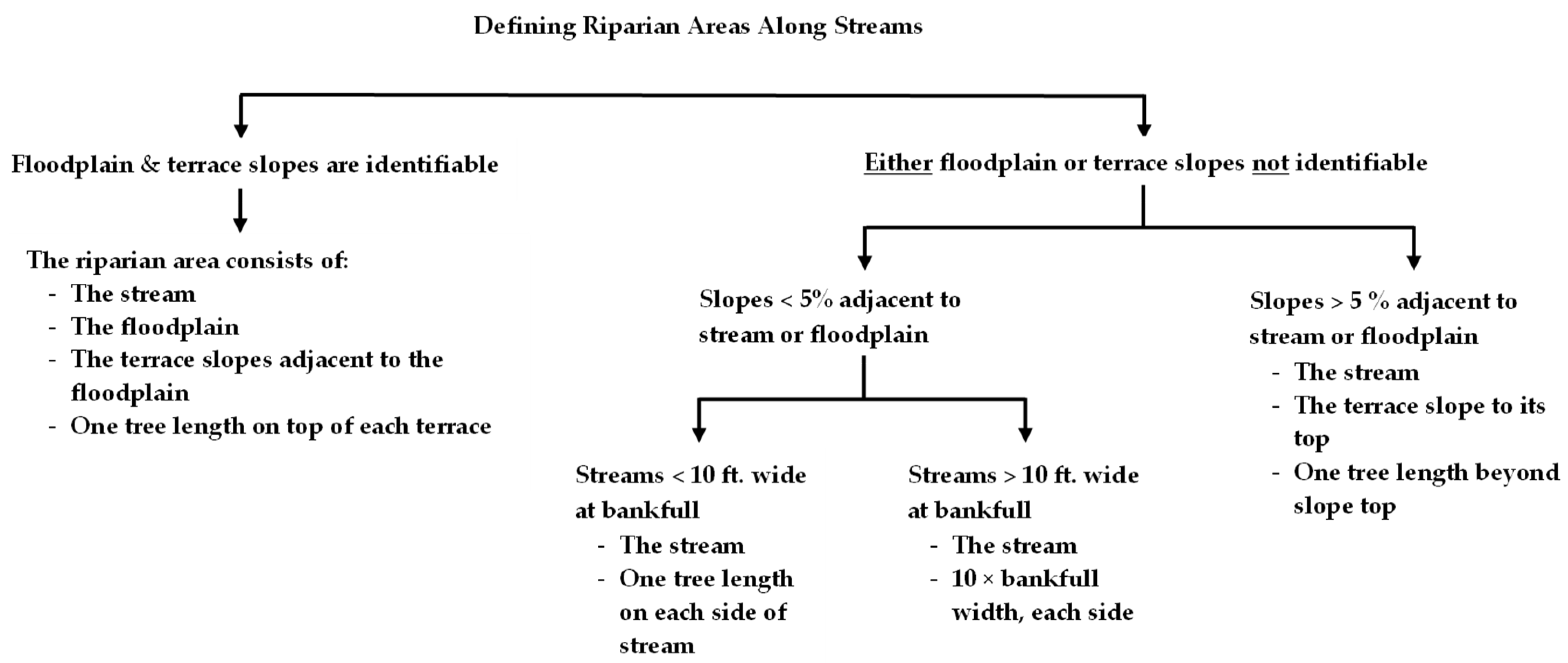
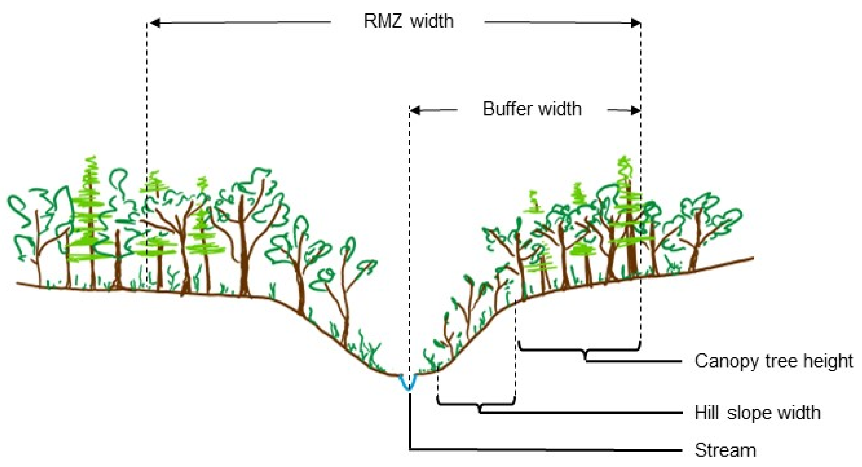
2.3.2. Functional Riparian Buffer Delineations

Ilhardt et al. [24] defined a variable-width, functional buffer as the stream, floodplain, terrace slope, and one-tree length from the top of the terrace slope (Figure 1). In this context, the term ‘terrace’ refers to abandoned floodplains that occur at a higher elevation than the active floodplain, and ‘terrace slope’ refers to the transitional land surface between the active floodplain and the higher terrace or upland area [24]. The majority of first- and second-order streams do not have established floodplains and terraced slopes. Rather than a ‘terrace slope’, these lower order streams have a ‘hill slope’. Using the “Ridge Finder” tool [18] developed using ArcGIS Pro 2.5.1 and R [38], we identified the floodplain (if present) and the upland boundary of the hill slope (i.e., where it transitions to the upland surface) along the selected first- and second-order streams. For example, in deeply V-shaped stream valleys, we used geomorphic indicators such as the upland extent of hillslope slumping to define the hill slope upper boundary, following guidance by Ilhardt et al. [24]. We furthermore delineated the horizontal width of an average tree height from the hill slope upper boundary, using the local FIA canopy data for each watershed. In the instances where no floodplain and hill slope development are present or when hill slope gradient is <5%, the buffer width of a functional RMZ was determined by the average canopy tree height [24]. Once this functional RMZ was delineated around the selected stream networks, the land areas representing this buffer for first- and second-order streams within a network were calculated through ArcGIS, as well as their ratio to the total watershed area.

2.3.3. State-Specific RMZ Delineation

Within the U.S., RMZ guidelines and buffer delineations are unique to each state (Table S2). Washington, Oregon, Idaho, California, and West Virginia have regulatory state RMZ guidelines, while Wisconsin, Michigan, Pennsylvania, New York, Vermont, New Hampshire, and South Carolina have quasi-regulatory state RMZ guidelines. Minnesota, Mississippi, Arkansas, Arizona, and Wyoming have voluntary state RMZ guidelines [19]. Five of the 17 states have separate guidelines for fish-bearing streams, and therefore, state stream network GIS files were used to identify those fish-bearing streams. Following state guidelines, RMZs were delineated for the three selected stream networks within watersheds using ArcGIS Pro 2.5.1 per methodologies developed by [18]. Thereafter, the RMZs for first- and second-order streams within a network were isolated and their respective land area allocations were recorded.

2.3.4. Standardizing RMZs and Calculating RMZ Widths

Standardization of RMZs was required since streams selected for the analysis were of differing lengths, and thus a per unit measurement was required for comparing between and amongst stream orders. Therefore, areas for the functional and state-specific RMZs were standardized to their respective stream lengths according to the following equation (Equation (2)).
RMZ   width = RMZ   area   ( m 2 ) Stream   length   ( m )
The RMZ width represents twice the average buffer width laterally on each side of the stream. For example, a stream length of 400 m having a state-specific RMZ of 20,000 m2 would have an RMZ width of 50 m, and the average state-specific buffer width for that stream is 25 m. The same calculation strategy was followed for determining the average buffer width for a functional RMZ.
The buffer width of a functional RMZ is the sum of the hill slope width and the average canopy tree height (Figure 3). In order to calculate the hill slope width for functional RMZs, we first divided the functional RMZ width by two to yield the average functional buffer width. Then the average canopy tree height for that watershed was deducted from the average functional buffer width to calculate the average hill slope width for a stream (Figure 3).

2.3.5. Comparing Land Area Differences between Functional and State-Specific RMZ Widths

To investigate the land area differences between a functional RMZ allocation and state-specific RMZ, a nonparametric two-way ANOVA was performed on the dataset [39,40]. The aligned rank test was performed on factors of states and stream orders. This allowed the investigation of land area differences between buffer allocation methods across states and stream orders. In addition, the hill slope width that represents the topography around streams was compared across states and stream orders. The ARTool package in R Studio [40] was used for the analysis.

2.3.6. Proportion of RMZs within a Watershed

As stated above, it was assumed that the RMZ width represents twice the average buffer width. The average RMZ width calculated for the selected stream networks within a watershed was also assumed to be representative of headwater streams within that watershed. This allowed the calculation of the percentage of watershed area those RMZs occupied through extrapolation.
The RMZ width for each order of headwater streams within a watershed was multiplied by its stream length. This provides the total area occupied by the RMZs along the order of the headwater streams within that watershed. After calculating the areas occupied by both orders, the percentage of watershed area for headwater RMZs was calculated as a proportion of the watershed area. For example, within a 240 km2 watershed, 19.2 km2 of headwater stream functional RMZ would comprise 8% of the watershed area. This calculation was performed for each RMZ allocation method and regional averages of percent watershed areas were calculated.

3. Results

3.1. Drainage Density

Drainage densities in study watersheds ranged between 0.49 km km−2 (0.30 miles miles−2) in South Carolina and 5.08 km km−2 (3.16 miles miles−2) in California (Table 1). The highest drainage density of 5.08 km km−2 was recorded in a watershed within the Mendocino National Forest in California, while the lowest drainage densities (0.49–0.61 km km−2) were located in woody wetland watersheds within the Hiawatha National Forest in Michigan and Marion National Forest in South Carolina. Between 61% and 96% of the stream networks within the study, watersheds were made up of headwater streams (Table 1).

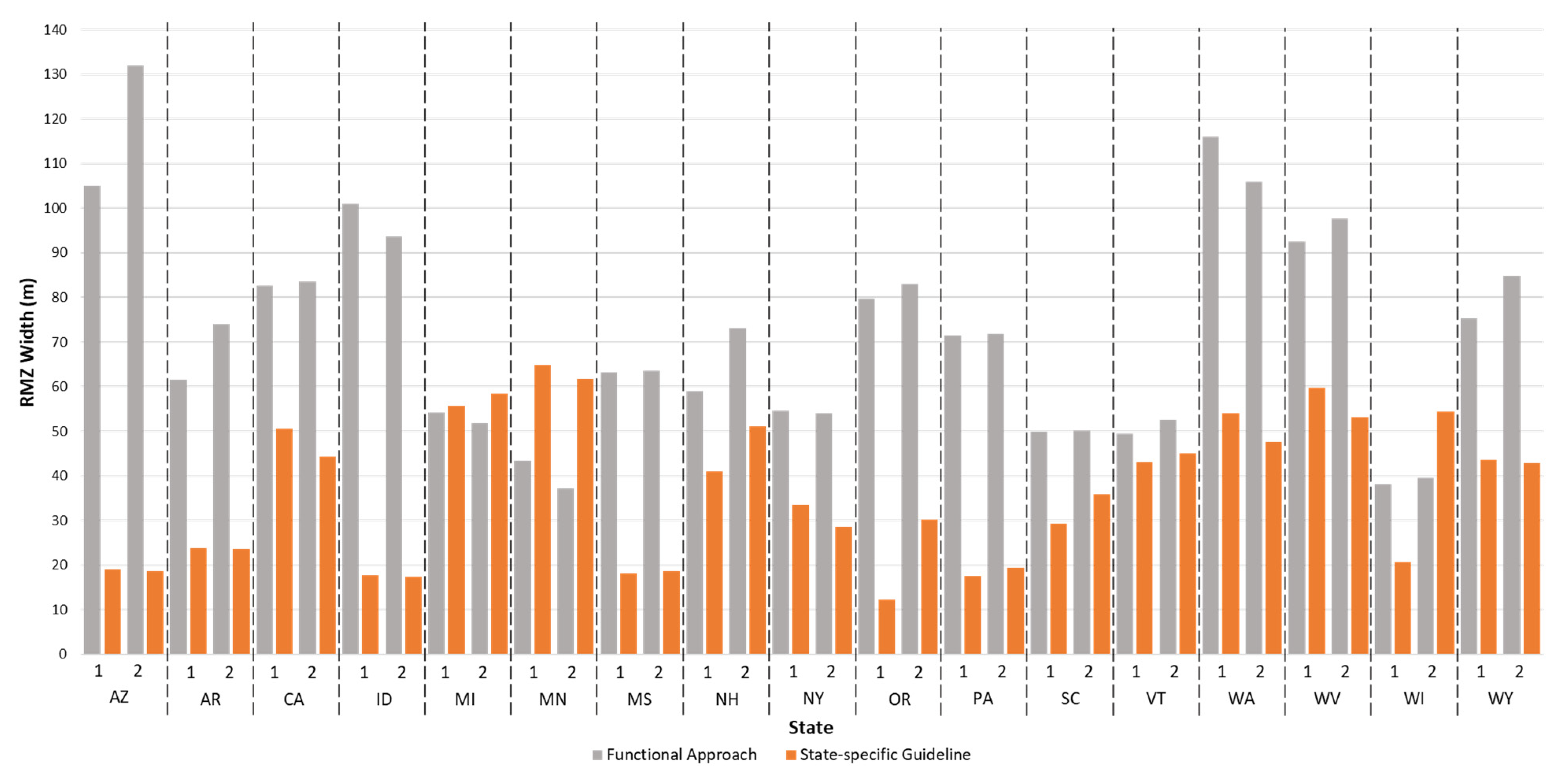
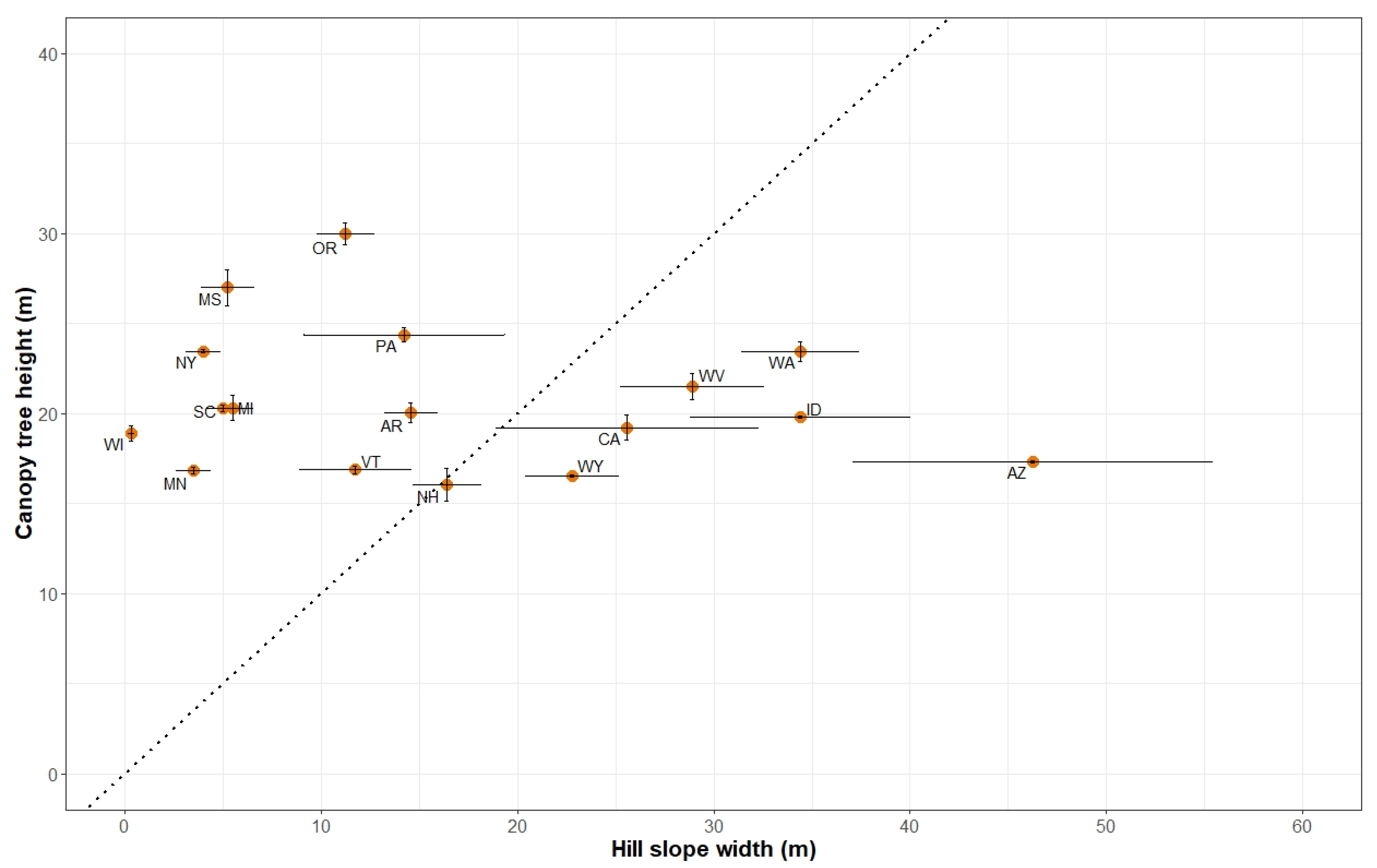
3.2. Functional RMZ Width Differences across States

The nonparametric factorial ANOVA test revealed that the functional RMZ widths varied significantly across states (p < 0.001) and stream orders (p = 0.0014). In watersheds in states such as Arizona and Washington, functional RMZ widths were over 100 m (328.08 ft.) along both stream orders, with median functional buffer widths greater than 50 m (164.04 ft.). Study watersheds in states such as Minnesota and Wisconsin had functional RMZ widths extending less than 50 m (164.04 ft.), with median functional buffer widths of less than 25 m (82.02 ft.) (Figure 4).
The ANOVA test for the assessment of hill slope width provided a topographic comparison of stream hill slopes across the study watersheds within states. Significant differences in delineated hill slopes existed across states (p < 0.001). The hill slope width was greatest along streams in the study watersheds of Arizona, Washington, Idaho, West Virginia, Wyoming, and California. For instance, along second-order streams in study watersheds of Arizona, the median distance was 50 m and extended up to 100 m. The functional RMZ width along the headwaters of study watersheds within these states was heavily influenced by the hill slope width (Figure 5). Headwater streams in study watersheds of Wisconsin showed no hill slope development, indicating very low topographic relief within sampled watersheds, which is exemplified by the 0 m median hill slope width. The median hill slope width ranged between 0 and 12 m (0–40 ft.) in the study watersheds of Michigan, Minnesota, Mississippi, South Carolina, New York, Oregon, Vermont, and Pennsylvania. The canopy tree height was a strong influence in determining the functional RMZ width along headwater streams of study watersheds within these states (Figure 5).

3.3. State-Specific RMZ Width Differences across States

The land area dedicated to state-specific RMZ widths along headwater streams showed significant differences across states (p < 0.001). There was also a significant difference between the land area between first- and second-order streams as delineated by state-specific RMZ widths across states (p = 0.029), in which second-order streams included more land area than first-order streams within the RMZ. State-specific RMZs allocated more land area along headwater streams in the study watersheds of the Great Lake states, which is exemplified by the study watersheds of Minnesota, where the widest state-specific RMZ widths were documented, extending up to 90 m (295.28 ft.) across the stream, or approximately a 45 m (147.64 ft.) buffer width (Figure 4). Significant differences in land area for state-specific RMZ allocations were also evident between first- and second-order streams in the study watersheds of Oregon and Wisconsin, in which the RMZ delineated more land area along second-order streams than first-order streams. Conversely, in the study watersheds of West Virginia, state-specific RMZs delineated more land area along first-order streams than second-order streams (Figure 4).

3.4. Comparison of Land Area Allocation between a Functional RMZ and a State-Specific RMZ

There was a significant difference in land area allocations between a functional RMZ and a state-specific RMZ between states (p < 0.0001). First- and second-order streams in the study watersheds of Minnesota and second-order streams in the study watersheds of Wisconsin are allocated more land area using state-specific RMZs when compared to a functional RMZ. The median deviation of the RMZ width was over 14 m (45.93 ft.) for second-order streams in the study watersheds of Wisconsin, while in the study watersheds of Minnesota the deviations were over 25 m (82.02 ft.) for both stream orders (Figure 4). The median functional RMZ width and state-specific RMZ width delineated along headwater streams in the study watersheds of Michigan were comparable to each other, showing deviations of only 5 m (16.40 ft.) (Figure 4). Functional RMZ widths in the study watersheds of Arizona and Idaho allocated over 75 m (246.06 ft.) and the study watersheds of Oregon, Pennsylvania, and Washington allocated over 50 m (164.04 m) across headwater streams than their respective state-specific RMZ widths.

3.5. Riparian Buffer Areas in Watersheds

When comparing the USFS functional method with state-specific guidelines, the functional method allocated more area as riparian in all regions except for the study watersheds of the Great Lakes states of Michigan, Minnesota, and Wisconsin, where average state-specific RMZ widths were wider in the study watersheds of Minnesota and Wisconsin and only slightly more in Michigan. Functional RMZs made up between 2% and 31% of the watershed area, whereas state-specific RMZs occupied between 1% and 23% of the watershed area within the study watersheds (Table 1). Overall, the highest percent watershed area delineated was 31% in the North Fork Creek watershed within the Mendocino National Forest in California, while the lowest percent watershed area was 1% in the forested wetlands in South Carolina and the Hiawatha National Forest in Michigan. In the study watersheds of Washington, California, Arizona, Oregon, Mississippi, Idaho, West Virginia, Michigan, New York, and Vermont ≥10% of the watershed was made up of functional RMZs, whereas state-specific RMZs only exceeded 10% of the watershed area in the study watersheds of Michigan (11%), Washington (18%), and California (23%).

4. Discussion

This study investigated and contrasted riparian buffer delineation techniques on headwater streams across 17 timber producing states of the contiguous U.S. The USFS functional riparian buffer method [24] that incorporates local topography and regional forest structure was compared with riparian buffers defined using state-specific regulations or voluntary guidelines. The functional RMZ is delineated based on near-stream topography and forest structure and is designed to encompass the zone of greatest efficacy for riparian functions such as stream shading, streambank integrity, pollutant filtering, and large wood and organic material contributions to the aquatic ecosystem [2,25,26,41]. This functional approach incorporates stream channel topography, including adjacent hill slopes that are easily erodible, to ensure bank stability. With an additional canopy tree height, laterally extending from the stream, it seeks to incorporate functions of, but not limited to shade, stream temperature regulation, allochthonous inputs of fine and coarse woody debris, and wildlife habitat [9,25,26].
Assigning the “just right” RMZ is an important management decision considering the high density of first- and second-order streams in working forested landscapes, and consequentially the potentially large area of forest land that would be precluded from land management activities. The practice of delineating the RMZ needs to strike a balance, neither undermining riparian protection nor creating an inordinate economic burden to the landowner.

4.1. State-Wide Differences in Functional RMZ Delineations

The functional RMZ delineation identifies hill slope width along the lateral widths of a stream, which varies between states. This buffer allocation method also accounts for the vertical forest structure adjacent to streams. It should also be noted that these sampled watersheds are not representative of the topography of those states and that terrain characteristics may be watershed specific. The median hill slope width was ≥22 m (72.18 ft.) in study watersheds located in states such as Arizona, Idaho, Washington, West Virginia, Wyoming, and California, and this was reflected by the wider functional RMZ widths for these states. Similarly, study watersheds in Oregon also displayed a wide functional riparian width along headwater streams, which was influenced to a large degree by the average canopy tree heights of the Douglas-fir forest types. The study watersheds in Northeastern and Southeastern states were comparable to each other with moderate hill slope widths (0–12 m (0–39.37 ft.)), except in the West Virginia study catchments where wide hill slope widths were observed in the mountainous Monongahela National Forest. The study watersheds in the Great Lakes states of Minnesota and Michigan also displayed moderate hill slope widths along first- and second-order streams. Headwater streams in the study watersheds of Wisconsin displayed no hill slope development, indicating that the functional RMZ within its watersheds was determined only by its average canopy tree height of roughly 20 m (65.62 ft). Thus, this variable-width RMZ reflects both the topography around the streams through the hill slope development and forest structural characteristics through the average canopy tree height.

4.2. Comparing State Prescribed RMZs with Functional RMZs

Comparisons between the state-specific RMZs and functional RMZs revealed that in the study watershed of Michigan, the combined topography and forest structure represented by the functional RMZ are reflected in their state-specific RMZ prescriptions. The Great Lake states of Michigan and Minnesota, along with the southeastern state of West Virginia, allocated the widest buffers around headwater streams in their state-specific prescriptions, whereas states such as Arkansas, Arizona, Idaho, Mississippi, Pennsylvania, and Oregon prescribed the narrowest buffers compared to other states. When comparing these state-specific RMZs to their functional RMZ counterparts, functionally defined buffers in the study watersheds of Minnesota comprised less land area than if they were delineated using state-prescribed guidelines, whereas the study watersheds in states such as Arizona, Idaho, and Oregon would require more riparian land area protected using the functional allocation approach compared to existing state guidelines.
Numerous synthesis studies of riparian buffer efficacy have noted that the influence on buffer functions such as pollutant filtration and in-stream temperature mitigation is sensitive to buffer width. In a meta-data analysis of a riparian efficacy study by [9], riparian buffers between 10 and 30 m (32.81–98.43 ft.) trapped sediment with an efficiency of between 65% and 85%. Thus, this is a useful standard by which to compare state buffer prescriptions. Groom et al. [42] reported for first- to third-order streams within the Coastal Range Forests of Oregon that RMZs with 15.24–21.34 m (50–70 ft.) of buffer width registered an average increase of 0.7 °C in maximum stream temperature between pre- and post-harvest periods, compared with no change for wider buffer widths ranging from 30.48 to 53.34 m (100–175 ft.). Changes in stream temperature can have significant impacts on trout habitat [43] and increases in sedimentation can have adverse impacts on aquatic habitat for both macro and micro invertebrate communities [44,45]. In this context, the state-specific RMZ prescriptions for Arizona, Idaho, and Mississippi are ≤10 m (32.81 ft.), which may not properly buffer sediment runoff or increased temperatures from forest operations within these watersheds. Given that the study watersheds within Arizona and Idaho displayed high topographic relief with wide hill slope widths, riparian buffers required to regulate sedimentation in this context may exceed 30 m (~100 ft.) in watersheds with similar topography. Similarly, in the study watersheds of Washington and Oregon, state-specific guidelines define fixed-width RMZs for non-fish-bearing streams that are ≤15 m (50 ft.). Because headwater streams in the steep and mountainous Pacific Northwest region typically have wide hill slope widths, particularly in Washington, the state-specific RMZ prescriptions for these states do not account for the key elements used in functional RMZ delineations to protect water quality and ecosystem integrity.
Functional RMZs delineated from topography and forest characteristics usually result in RMZs that exceed buffer prescriptions commonly used in the U.S., whether defined as fixed or variable width buffers in their state BMP guides. Such is the case in this study for most states, except for study watersheds in the Great Lakes states, characterized by low topographic relief. Forested watersheds with similar topography and forest structure as represented by the study watersheds in the Great Lakes states will likely experience opportunity costs due to state-specific guidelines that define riparian buffers greater than those identified by a functional RMZ. However, in watersheds where state-specific RMZs fail to capture wide hill slope widths on steeper landscapes (ex: West and Pacific Northwest watersheds), they should ensure that riparian buffers incorporate full hill slope widths where the soil is more susceptible to erodibility.

4.3. Proportion of RMZs in Watersheds

Headwater streams dominated channel networks by their cumulative stream lengths in all watersheds. They represented between 61% and 96% of entire stream networks across the study watersheds. The study watersheds in California, Washington, Michigan, Oregon, New York, and Arizona recorded some of the highest watershed stream densities in the study with an average range between 1.99 and 3.84 km km−2 (1.24–2.39 miles miles−2) while the study watersheds in Great Lakes states recorded some of the lowest average watershed drainage densities that ranged between 1.05 and 1.07 km km−2 (0.65–0.66 miles miles−2). These values are consistent with other studies from these regions [46,47,48,49,50].
High drainage densities within watersheds are generally correlated with areas of high topographic relief [47]. The study watersheds in Arizona, Washington, and California displayed wide hill slope widths with high slope gradients as well as high drainage densities. High surface flow rates in high drainage density watersheds with steep slopes could make land adjacent to streams more susceptible to erosion [51]. Wider buffer widths may allow for more infiltration time in these areas and reduce the risk of erosion. Therefore, a functional RMZ that identified wide lateral slope widths of headwater streams may be more appropriate for streams in these watersheds.
Headwater RMZs in the study watersheds of Washington, California, Arizona, and Oregon accounted for the highest proportions of watersheds. This might be due to the high drainage densities, topographic relief, and wider hill slopes observed within these watersheds. Functional RMZs resulted in the largest proportion of land delineated as riparian in comparison to state-specific RMZs in all regions except in the study watersheds in the Great Lakes states. This was due to the low drainage densities, lack of topographic relief, and little to no hill slope development. Lippke et al. [52] estimated that 14.8% of commercial forest land in western Washington would fall within a riparian buffer of 45.72 m (150 ft.) for fish-bearing streams (classes I to III), 30.48 m (100 ft.) for class IV streams, and 15.24 m (50 ft.) for class V streams. These buffer parameters reflected state-specific RMZ prescriptions during the time of this research. When extrapolated to represent all headwater streams, the percent acreage of riparian areas represented approximately 11% of the commercial forest. Our study recorded an average area of 12% delineated for state-prescribed RMZs along headwaters for the study watersheds in the Olympic Peninsula in Washington. In a study conducted across the USDA Crossett Experimental Forest, University of Arkansas Forest, Ouachita National Forest, and Ozark National Forest, Kluender et al. [53] reported an average of 6.3% of forestland dedicated to all streams with a 20.12 m (66 ft.) fixed-width buffer. If extrapolated to the percent of headwater streams represented by both functional and state-specific RMZ delineation, the study watersheds in Arkansas dedicated approximately 5.8% of forestland to RMZs along headwaters.
Drainage density plays a key role in determining the proportion of the forestland delineated as RMZs in addition to the buffer allocation method used. As drainage densities within a watershed increase, the percent acreage of RMZs increases proportionately. Headwater streams tend to be under-represented by current NHD layers within forested watersheds where their actual densities may be higher than those represented by hydrographic datasets [4,5,6] and vice-versa. Field verification is therefore required and recommended when mapping headwater streams within working forests for management as this can have a significant impact on costs for allocating RMZs regardless of the buffer allocation method used.

4.4. Implications for Forest Managers

RMZs are an integral part of forestry BMPs for controlling sediment runoff and protecting other riparian values during and after forest operations. As accessibility and resolution of DETMs rapidly increase, the delineation and adaptation of variable-width buffers that consider topography is becoming easier to implement on any given forest landscape. Riparian delineation tools used for this research (‘Ridge Finder’) as well as the RBDMv6x Tool developed by Abood et al. [54] may be used for allocating variable width buffers such as the USFS functional riparian method. Regardless of whether RMZs are regulated or voluntary, it is important to define buffers around headwater streams to protect and preserve the integrity of aquatic and riparian ecosystems. As this study reveals, the percentage of the area designated as riparian areas along headwater streams can range from as low as 1.5% to nearly 25%. Jayasuriya et al. [50] estimated that riparian areas in the Catskill region of New York represented a stumpage value for northern hardwoods of over USD 3707 ha−1 (USD 1500 ac−1). They reported that if RMZ harvesting restrictions limited removals to 1MBF ac−1, the opportunity cost of allocating RMZs along headwater streams accounted for 7% of the total timber revenue for that timberland. Lakel et al. [55] recorded values from as little as USD 135 ha−1 (USD 55 ac−1) to USD 3128 ha−1 (USD 1266 ac−1) for stands that were mainly composed of loblolly pine and white oak in an efficacy study estimating the minimum riparian width along first-order streams in watersheds of the Piedmont Plateau in Virginia. Considering differences in forest cover types across the various states in this study, the RMZ can hold a substantial amount of valuable timber [50,55,56,57]. Thus, partial harvesting management options such as single tree selection, without compromising riparian functions, can be allowed within RMZs to decrease the cost of allocating riparian buffers along headwater streams.

4.5. Study Limitations

The sampled watersheds included in this study were limited to public lands and, furthermore, only provide a fraction of the topography seen within a state and may not represent the topographic range seen across working forests within those states. Therefore, further research on terrain analysis that includes more watersheds distributed across a state is required to facilitate policy decisions related to revising or amending state-specific RMZ guidelines. In addition, the increasing attention received for ‘tailored riparian area protection’ highlights the importance of investigating other riparian functions in addition to water quality protection, such as (but not limited to) biogeochemical cycling, groundwater recharge, biomass accumulation, and wildlife habitat—all of which could influence RMZ guidelines.

5. Conclusions

Headwater streams dominate channel networks, comprising between 61% and 96% of the entire stream networks in all watersheds examined in this study. The high density of headwater streams within working forests poses challenges to forest managers seeking to conduct financially viable timber operations while simultaneously protecting riparian and aquatic ecosystem functions. At high stream densities, delineating the “just right” riparian buffer around headwater streams becomes a consequential management decision due to the risks of overestimating or underestimating appropriate riparian areas using different buffer allocation methods. If forest managers choose to use functional RMZ guidelines, they should expect topography and forest structure to strongly influence the RMZ area.

Supplementary Materials

The following supporting information can be downloaded at: https://www.mdpi.com/article/10.3390/f13091509/s1, Table S1: Summary of forest composition in study watersheds across the United States. Table S2: State-specific riparian buffer allocation guide for selected states in the study. The buffer indicates the lateral distance of the riparian allocation on one side of the stream.

Author Contributions

M.T.J.’s contribution to the manuscript includes conceptualization, methodology, validation, formal analysis, investigation, data curation, writing—original draft, writing—review and editing, visualization, project administration, and funding acquisition. R.H.G.’s contributions include conceptualization, methodology, validation, writing—original draft, writing—review and editing, visualization, supervision, project administration, and funding acquisition. J.C.S.’s contributions include writing—original draft, writing—review and editing, visualization, supervision, and funding acquisition. All authors have read and agreed to the published version of the manuscript.

Funding

This research was funded by a grant from the McIntire-Stennis program of the U.S. Department of Agriculture (USDA) (Grant No.: 1139513-79903-35) National Institute of Food and Agriculture (NIFA) and additional financial support from SUNY College of Environmental Science and Forestry (SUNY ESF), USA.

Data Availability Statement

Publicly available datasets were analyzed in this study. All data sources used for the analysis have been described under the section Data Sources along with their weblinks except when referring to individual state GIS datasets.

Conflicts of Interest

The authors declare no conflict of interest.

References

  1. Shreve, R.L. Statistical Properties of Stream Lengths. J. Geol. 1969, 77, 397–414. [Google Scholar] [CrossRef]
  2. Naiman, R.J.; Décamps, H.; McClain, M.E. Riparia: Ecology, Conservation, and Management of Streamside Communities; Elsevier Academic Press: Cambridge, MA, USA, 2005; ISBN 9780080470689. [Google Scholar]
  3. Opperman, J.J.; Moyle, P.B.; Larson, E.W.; Florsheim, J.L.; Manfree, A.D. Floodplains. Processes and Management for Ecosystems; University of California Press: Oakland, CA, USA, 2017. [Google Scholar]
  4. Baker, M.E.; Weller, D.E.; Jordan, T.E. Effects of Stream Map Resolution on Measures of Riparian Buffer Distribution and Nutrient Retention Potential. Landsc. Ecol. 2007, 22, 973–992. [Google Scholar] [CrossRef]
  5. Brooks, R.T.; Colburn, E.A. Extent and Channel Morphology of Unmapped Headwater Stream Segments of the Quabbin Watershed, Massachusetts. JAWRA J. Am. Water Resour. Assoc. 2011, 47, 158–168. [Google Scholar] [CrossRef]
  6. Elmore, A.J.; Julian, J.P.; Guinn, S.M.; Fitzpatrick, M.C. Potential Stream Density in Mid-Atlantic U.S. Watersheds. PLoS ONE 2013, 8, e74819. [Google Scholar] [CrossRef] [PubMed]
  7. Binkley, D.; Brown, T.C. Forest Practices as Nonpoint Sources of Pollution in North America. J. Am. Water Resour. Assoc. 1993, 29, 729–740. [Google Scholar] [CrossRef]
  8. Phillips, M.J.; Blinn, C.R. Best Management Practices Compliance Monitoring Approaches for Forestry in the Eastern United States. Water Air Soil Pollut. Focus 2004, 4, 263–274. [Google Scholar] [CrossRef]
  9. Sweeney, B.W.; Newbold, J.D. Streamside Forest Buffer Width Needed to Protect Stream Water Quality, Habitat, and Organisms: A Literature Review. JAWRA J. Am. Water Resour. Assoc. 2014, 50, 560–584. [Google Scholar] [CrossRef]
  10. Lakel, W.A.; Aust, W.M.; Bolding, M.C.; Dolloff, C.A.; Keyser, P.; Feldt, R. Sediment Trapping by Streamside Management Zones of Various Widths after Forest Harvest and Site Preparation. For. Sci. 2010, 56, 541–551. [Google Scholar]
  11. Ward, J.M.; Jackson, C.R. Sediment Trapping Within Forestry Streamside Management Zones: Georgia Piedmont, USA. JAWRA J. Am. Water Resour. Assoc. 2004, 40, 1421–1431. [Google Scholar] [CrossRef]
  12. Chizinski, C.J.; Vondracek, B.; Blinn, C.R.; Newman, R.M.; Atuke, D.M.; Fredricks, K.; Hemstad, N.A.; Merten, E.; Schlesser, N. The Influence of Partial Timber Harvesting in Riparian Buffers on Macroinvertebrate and Fish Communities in Small Streams in Minnesota, USA. For. Ecol. Manag. 2010, 259, 1946–1958. [Google Scholar] [CrossRef]
  13. Jackson, R.C.; Batzer, D.P.; Cross, S.S.; Haggerty, S.M.; Sturm, C.A. Headwater Streams and Timber Harvest: Channel, Macroinvertebrate, and Amphibian Response and Recovery. For. Sci. 2007, 53, 356–370. [Google Scholar]
  14. Lee, P.; Smyth, C.; Boutin, S. Quantitative Review of Riparian Buffer Width Guidelines from Canada and the United States. J. Environ. Manag. 2004, 70, 165–180. [Google Scholar] [CrossRef] [PubMed]
  15. Jayasuriya, M.T.; Stella, J.C.; Germain, R.H. Can Understory Plant Composition and Richness Help Designate Riparian Management Zones in Mesic Headwater Forests of the Northeastern United States? J. For. 2021, 119, 574–588. [Google Scholar] [CrossRef]
  16. Blinn, C.R.; Kilgore, M.A. Riparian Management Practices: A Summary of State Guidelines. J. For. 2001, 99, 11–17. [Google Scholar]
  17. Castelle, A.J.; Johnson, A.W. Riparian Vegetation Effectiveness; National Council for Air and Stream Improvement, Inc.: Cary, NC, USA, 2000. [Google Scholar]
  18. Jayasuriya, M.T. The Effects Of Riparian Management Zone Delineation On Timber Value And Ecosystem Services In Diverse Forest Biomes Across The United States. Ph.D. thesis, The State University of New York College of Environmental Science and Forestry, Syracuse, NY, USA, 2020. [Google Scholar]
  19. Cristan, R.; Michael Aust, W.; Chad Bolding, M.; Barrett, S.M.; Munsell, J.F. National Status of State Developed and Implemented Forestry Best Management Practices for Protecting Water Quality in the United States. For. Ecol. Manag. 2018, 418, 73–84. [Google Scholar] [CrossRef]
  20. Bren, L.J. The Geometry of a Constant Buffer-Loading Design Method for Humid Watersheds. For. Ecol. Manag. 1998, 110, 113–125. [Google Scholar] [CrossRef]
  21. Tomer, M.D.; James, D.E.; Isenhart, T.M. Optimizing the Placement of Riparian Practices in a Watershed Using Terrain Analysis. J. Soil Water Conserv. 2003, 58, 198–206. [Google Scholar]
  22. Tiwari, T.; Lundström, J.; Kuglerovà, L.; Laudon, H.; Öhman, K.; Ågren, A.M. Cost of Riparian Buffer Zones: A Comparison of Hydrologically Adapted Site-Specific Riparian Buffers with Traditional Fixed Widths. Water Resour. Res. 2016, 52, 1056–1069. [Google Scholar] [CrossRef]
  23. Kuglerová, L.; Jansson, R.; Ågren, A.; Laudon, H.; Malm-Renöfält, B. Groundwater Discharge Creates Hotspots of Riparian Plant Species Richness in a Boreal Forest Stream Network. Ecol. Soc. Am. 2014, 95, 715–725. [Google Scholar] [CrossRef]
  24. Ilhardt, B.L.; Verry, E.S.; Palik, B.J. Defining Riparian Areas. In Riparian Management in Forests in the Continental Eastern United States; Lewis Publishers: Boca Raton, FL, USA, 2000; pp. 23–42. [Google Scholar]
  25. Swanson, F.J.; Gregory, S.V.; Sedell, J.R.; Campbell, A.G. Land-Water Interactions: The Riparian Zone. In Analysis of Coniferous Forest Ecosystems in the Western United States; Edmonds, R.L., Ed.; Hutchinson Ross Publishing Co.: Stroudsburg, PA, USA, 1982; pp. 267–291. [Google Scholar]
  26. Gregory, S.V.; Swanson, F.J.; McKee, W.A.; Cummins, K.W. An Ecosystem Perspective of Riparian Zones. Bioscience 1991, 41, 540–551. [Google Scholar] [CrossRef]
  27. Richardson, J.S.; Naiman, R.J.; Bisson, P.A. How Did Fixed-Width Buffers Become Standard Practice for Protecting Freshwaters and Their Riparian Areas from Forest Harvest Practices? Freshw. Sci. 2012, 31, 232–238. [Google Scholar] [CrossRef]
  28. Flores, L.; Larrañaga, A.; Díez, J.; Elosegi, A. Experimental Wood Addition in Streams: Effects on Organic Matter Storage and Breakdown. Freshw. Biol. 2011, 56, 2156–2167. [Google Scholar] [CrossRef]
  29. Diez, J.R.; Elosegi, A.; Pozo, J. Woody Debris in North Iberian Streams: Influence of Geomorphology, Vegetation, and Management. Environ. Manag. 2001, 28, 687–698. [Google Scholar] [CrossRef]
  30. Harmon, M.E.; Franklin, J.F.; Swanson, F.J.; Sollins, P.; Gregory, S.V.; Lattin, J.D.; Anderson, N.H.; Cline, S.P.; Aumen, N.G.; Sedell, J.R.; et al. Advances in Ecological Research Ecology of Coarse Woody Debris in Temperate Ecosystems. Adv. Ecol. Res. 1986, 15, 133–302. [Google Scholar]
  31. U.S. Bureau of Economic Analysis (BEA). Available online: https://www.bea.gov/ (accessed on 3 September 2022).
  32. OpenTopography. Available online: https://opentopography.org/ (accessed on 5 July 2020).
  33. USDA Forest Service FSGeodata Clearinghouse-Download National Datasets. Available online: https://data.fs.usda.gov/geodata/edw/datasets.php (accessed on 3 September 2022).
  34. FIA DataMart FIADB_1.9.0: Home. Available online: https://apps.fs.usda.gov/fia/datamart/datamart.html (accessed on 3 September 2022).
  35. Munsell, J.F.; Germain, R.H. Woody Biomass Energy: An Opportunity for Silviculture on Nonindustrial Private Forestlands in New York. J. For. 2007, 105, 398–402. [Google Scholar] [CrossRef]
  36. Strahler, A.N. Dynamic Basis of Geomorphology. GSA Bull. 1952, 63, 923–938. [Google Scholar] [CrossRef]
  37. Strahler, A.N. Dimensional Analysis Applied to Fluvially Eroded Landforms | GSA Bulletin | GeoScienceWorld. GSA Bull. 1958, 69, 279–300. [Google Scholar] [CrossRef]
  38. R Core Team R: A Language and Environment for Statistical Computing. R Foundation for Statistical Computing. Available online: https://www.r-project.org/ (accessed on 17 March 2020).
  39. Wobbrock, J.; Findlater, L.; Gergle, D.; Higgins, J. The Aligned Rank Transform for Nonparametric FactorialAnalyses Using Only ANOVA Procedures. In Proceedings of the ACM Conference on Human Factors in Computing Systems (CHI ’11), Vancouver, BC, Canada, 7–12 May 2011; pp. 143–146. [Google Scholar]
  40. Kay, M.; Elkin, L.A.; Higgins, J.J.; Wobbrock, J.O. ARTool: Aligned Rank Transform for Nonparametric Fac-torial ANOVAs. R package version 0.11.1, 2021. for Statistical Computing. Available online: https://github.com/mjskay/ARTool (accessed on 17 March 2020).
  41. Stella, J.C.; Kui, L.; Golet, G.H.; Poulsen, F. A Dynamic Riparian Forest Structure Model for Predicting Large Wood Inputs to Meandering Rivers. Earth Surf. Process. Landf. 2021, 46, 3175–3193. [Google Scholar] [CrossRef]
  42. Groom, J.D.; Dent, L.; Madsen, L.J.; Fleuret, J. Response of Western Oregon (USA) Stream Temperatures to Contemporary Forest Management. For. Ecol. Manag. 2011, 262, 1618–1629. [Google Scholar] [CrossRef]
  43. Beschta, R.L.; Bilby, R.E.; Brown, G.W.; Holtby, L.B.; Hofstra, T.D. Stream Temperature and Aquatic Habitat: Fisheries and Forestry Interactions; University of Washington: Seattle, WA, USA, 1987. [Google Scholar]
  44. Newbold, J.D.; Erman, D.C.; Roby, K.B. Effects of Logging on Macroinvertebrates in Streams With and Without Buffer Strips. Can. J. Fish. Aquat. Sci. 1980, 37, 1076–1085. [Google Scholar] [CrossRef]
  45. Davies, P.E.; Nelson, M. Relationships between Riparian Buffer Widths and the Effects of Logging on Stream Habitat, Invertebrate Community Composition and Fish Abundance. Mar. Freshw. Res. 1994, 45, 1289–1309. [Google Scholar] [CrossRef]
  46. Kuska, J.; Arra, V.A.L. Use of Drainage Patterns and Densities to Evaluate Large Scale Land Areas for Resource Management. J. Environ. Syst. 1973, 3, 85. [Google Scholar] [CrossRef]
  47. Patton, P.C.; Baker, V.R. Morphometry and Floods in Small Drainage Basins Subject to Diverse Hydrogeomorphic Controls. Water Resour. Res. 1976, 12, 941–952. [Google Scholar] [CrossRef]
  48. Montgomery, D.R.; Dietrich, W.E. Source Areas, Drainage Density, and Channel Initiation. Water Resour. Res. 1989, 25, 1907–1918. [Google Scholar] [CrossRef]
  49. Wemple, B.C.; Swanson, F.J.; Jones, J.A. Forest Roads and Geomorphic Process Interactions, Cascade Range, Oregon. Earth Surf. Process. Landf. 2001, 26, 191–204. [Google Scholar] [CrossRef]
  50. Jayasuriya, M.T.; Germain, R.H.; Bevilacqua, E. Stumpage Opportunity Cost of Riparian Management Zones on Headwater Streams in Northern Hardwood Timberlands. For. Sci. 2019, 65, 108–116. [Google Scholar] [CrossRef]
  51. EnviroAtlas. Stream Density How Can I Use This Information? 2015. Available online: https://enviroatlas.epa.gov/enviroatlas/datafactsheets/pdf/ESN/Streamdensity.pdf. (accessed on 3 September 2022).
  52. Lippke, B.; Bare, B.B.; Xu, W.; Mendoza, M. An Assessment of Forest Policy Changes in Western Washington. J. Sustain. For. 2002, 14, 63–94. [Google Scholar] [CrossRef]
  53. Kluender, R.A.; Weih, R.; Corrigan, M.; Pickett, J. Assessing the Operational Cost of Streamside Management Zones. For. Prod. J. 2000, 50, 30–34. [Google Scholar]
  54. Abood, S.A.; Maclean, A.L.; Mason, L.A. Modeling Riparian Zones Utilizing DEMS and Flood Height Data. Photogramm. Eng. Remote Sens. 2012, 78, 259–269. [Google Scholar] [CrossRef]
  55. Lakel, W.A.; Aust, W.M.; Dolloff, C.A.; Keyser, P.D. Residual Timber Values within Piedmont Streamside Management Zones of Different Widths and Harvest Levels. For. Sci. 2015, 61, 197–204. [Google Scholar] [CrossRef]
  56. Ice, G.G.; Skaugset, A.; Simmons, A. Estimating Areas and Timber Values of Riparian Management on Forest Lands. J. Am. Water Resour. Assoc. 2006, 42, 115–124. [Google Scholar] [CrossRef]
  57. Jayasuriya, M.T.; Germain, R.H.; Wagner, J.E. Protecting Timberland RMZs through Carbon Markets: A Protocol for Riparian Carbon Offsets. For. Policy Econ. 2020, 111, 102084. [Google Scholar] [CrossRef]
Figure 1. Decision tree for delineating a “functional”-based riparian area [24].
Forests 13 01509 g001
Figure 2. Locations of selected watersheds within the contiguous United States.
Forests 13 01509 g002
Figure 3. Illustration of a cross section of a function RMZ along a headwater stream. The functional buffer width is the sum of the hill slope width and the average canopy tree height. In the absence of a hill slope development, the functional buffer width is represented by the average canopy tree height.
Forests 13 01509 g003
Figure 4. Riparian Management Zone (RMZ) widths of headwater streams across states in the U.S. This bar plot represents the average RMZ widths along first- and second-order streams for RMZs delineated using the USFS functional approach and state-specific RMZ guidelines or rules.
Forests 13 01509 g004
Figure 5. Relationship between the average canopy tree height and average hill slope along headwater streams of the study watersheds within 17 states. The diagonal reference line helps identify the variable that drives the width of a functional RMZ. The standard error (+/−) for each variable is represented by the error bars on the x and y axis.
Forests 13 01509 g005
Table 1. Statistics of sampled watersheds.
StateIDWatershed LocationAvg. Dominant/Co-dominant Tree Height (m)Drainage Density of Headwater Streams (km km−2) 1Avg. Headwater Stream Network Percentage (%) 2Percent Watershed Area (%)
FunctionalState RMZ
Arizona (AZ)Lookout LakesKaibab National Forest17.41.6670132
Moquitch Canyon17.42.3171213
Arkansas (AR)DardanelleMount Magazine State Park18.31.688083
OuachitaOzark National Forest21.61.418093
California (CA)North Fork CreekMendocino National Forest21.65.08763123
Smith Neck CreekTahoe National Forest16.52.5970178
Idaho (ID) (lower)Granite CreekBoise National Forest19.81.367392
Minneha Creek19.81.4584152
Michigan (MI)HiawathaHiawatha National Forest20.10.547022
OttawaOttawa National Forest21.62.61771111
Minnesota (MN)BurnsideBurnside State Forest16.51.237446
SuperiorSuperior State Forest17.10.866125
Mississippi (MS)Sugar-Coffee BogueBienville National Forest30.52.1477113
Rocky BranchHomochitto National Forest23.93.2772154
New Hampshire (NH)WM1White Mountains National Forest13.11.357965
WM218.91.427785
New York (NY)Huntington Wildlife ForestAdirondacks23.51.648074
Frost ValleyCatskills23.52.4373106
Oregon (OR)South Fork Cow CreekRouge River National Forest322.4973163
Thunder CreekUmpqua National Forest281.9878123
Pennsylvania (PA)FarnsworthAlleghany National Forest24.11.276882
Salmon Creek25.61.427472
South Carolina (SC)Echaw CreekMarion National Forest19.80.499621
Wedboo Creek210.618532
Vermont (VT)GM1Green Mountains National Forest16.21.7578108
GM217.41.637455
Washington (WA)Quilcene RiverOlympic National Forest25.32.4676226
Skokomish River21.63.17742818
West Virginia (WV)PocahontasMonongahela National Forest23.81.5574126
Pendleton19.21.346585
Wisconsin (WI)Taylor County WSChequamegon-Nicolet National Forest20.71.097634
Price County WS18.91.057633
Wyoming (WY)Fish CreekTeton National Forest16.51.398195
1 Drainage density is the ratio of the summed stream lengths within a catchment divided by the total catchment area. 2 Headwater stream network percentage is the ratio of summed headwater (first- and second-order) stream length to the total stream length within a catchment.
Publisher’s Note: MDPI stays neutral with regard to jurisdictional claims in published maps and institutional affiliations.

