Article

Ecological Response of Urban Forest Carbon Density to Site Conditions: A Case Study of a Typical Karst Mountainous Regions in Southwest China

1
College of Life Sciences, Guizhou University, Guiyang 550025, China
2
Collaborative Innovation Center for Mountain Ecology & Agro-Bioengineering, Guiyang 550025, China
*
Author to whom correspondence should be addressed.
Forests 2022, 13(9), 1484; https://doi.org/10.3390/f13091484
Submission received: 20 August 2022 / Revised: 10 September 2022 / Accepted: 11 September 2022 / Published: 14 September 2022
(This article belongs to the Section Forest Ecology and Management)

Abstract

:
Understanding the ecological constraints of limiting the magnitude and the allocation of carbon density is critical for executing adaptive forest management programs and upgrading the size of carbon sinks. Taking a typical karst mountainous region Guiyang City as a case study area, this study computed the biomass of different forest types using the volume–biomass equations and mapped the carbon density distribution of forests. Furthermore, the random forest algorithm and spatial autoregression model were adopted to reveal the effects of site conditions on carbon density in karst forests. The results indicate that the forest ecosystems of Guiyang City had a high carbon sequestration potential, and there was a significant difference in the carbon density of forests in terms of space dimensions. Road density, 0 cm cation exchange capacity, and soil parent materials were the dominant factors determining the spatial distribution of homogeneous units with different levels of carbon density. This study underlines the urgency adapting to the growing conditions of forests in terms of complex site conditions, and provides a scientific basis for optimizing forest management practices, to maintain their carbon sequestration capacity under urbanization pressure and fragile habitats.

1. Introduction

Forests occupy about 31% of the world’s land area, and over 86% of global vegetation carbon and 73% of global soil C pools are stored in varied forest ecosystems [1]. Owing to their huge carbon pool and high productivity, afforestation is considered a cost-effective strategy to enhance ecological functions, reduce global warming, and promote sustainable development [2]. Therefore, accurate estimation of biomass carbon storage has been a prerequisite and basis for assessing the capacity of forests to absorb carbon and mitigate climate change. The carbon density of forest is a key indicator of carbon sequestration, and its spatial patterns can mirror the relationship between the geographic environment and carbon storage to some extent [3]. Numerous studies have been conducted to calculate the biomass, carbon storage, and carbon density of forest, as well as its spatiotemporal distributions at various scales and regions in recent decades [4,5,6]. Up to date, a bottom-up inventory approach is frequently used to estimate forest vegetation carbon stocks, estimating the carbon stocks of forest ecosystems at different regional scales and then calculating the carbon stocks of forest ecosystems at nationwide scales [7]. Forest inventory is one of the most pragmatic and effective ways to evaluate regional forests for carbon sequestration [8]. However, the carbon sequestration capacity of forests depends on forest productivity, which is limited by the natural factors and management [9]. Consequently, investigating the relationship between carbon density and site conditions is of great necessity when assessing forest carbon sequestration.
The variabilities in carbon densities and their spatial distribution patterns strongly depend on the interactions of various environmental factors, such as climate, topography, soils, biology, and human activities, on forest biomass at a variety of timescales [10]. In addition, the important influencing factors of the forest’s potential to sequester carbon are different due to the intensity of disturbances and the ecological background condition [11,12]. To date, however, an analysis of how intricate site conditions impact carbon sequestration is still insufficient, especially in ecologically fragile zones [13].
The karst ecosystem restrained by karst geological settings is an ecologically fragile environment, which mainly covers the southwestern regions of China [14]. Southwest China is not only one of the largest karst areas in the world, but also has the largest karst forest composed of evergreen broadleaved forest and seasonal rainforest in China [15]. Due to the coupling of water-rock-soil-gas-organism and the binary three-dimensional geological structure, a karst forest has a significant carbon sink effect and plays an important role in the regional and global carbon cycles [16]. However, karst regions are characterized by fragmented habitat and low ecosystem stability that are susceptible to external disturbances, which promote the degradation of forests, increase the difficulty of vegetation restoration, and lead to fluctuations in the carbon sequestration and sink enhancement capacity in the area [13,17]. Studies have disclosed that the productivity and biomass of karst forests were generally lower than non-karst forests, leading to unequal carbon benefit levels, even in the same climatic zone [18]. Furthermore, most studies have acknowledged that the carbon sequestration capacity of an ecosystem is generally limited by the local geological background and human interferences [10,13]; nonetheless, the complexity of karst structure makes it arduous to carry out on-the-spot measurements, the influence of abiotic and biotic factors on karst forest carbon sequestration has not been adequately evaluated [19]. Because karst areas are sensitive to changes in the external environment, they are ideal places to study the relationship between the carbon cycle and the environment. Consequently, studies that perform the ecological response of carbon cycle to site conditions are intensely required, which are profitable to assess the contribution of the karst forest and build locally adapted forest management.
Located in southwest China’s hinterland, Guiyang City is a typical resource-dependent and low-carbon pilot city [18]. Due to high ecological sensitivity and extreme depletion of renewable resources, most of the forests have become degraded to varying degrees in karst regions [20]. Meanwhile, ecological restoration is being increasingly implemented worldwide and is deemed as a major strategy for counteracting this trend [2]. As is known to all, intricate relationships exist between variable site conditions and the forest carbon cycle in the process of constructing ecological civilization and low-carbon ecological cities, particularly in areas with unique geological contexts and fragile ecological foundations [21]. It provides an ideal study area to evaluate regional carbon stocks under the coupled effects of low-carbon development and ecologization.
Therefore, taking Guiyang Metropolitan Area as a case study, to quantitatively assess the carbon sequestration potential of karst urban forests and their ecological responses to site conditions, the objectives of this study were as follows: (1) to determine the carbon stocks and carbon density of different forest types; (2) to identify the spatial variability of carbon density; (3) to reveal the dominant site conditions affecting carbon density of karst urban forest and its effects on the efficiency of forest carbon sequestration production.

2. Materials and Methods
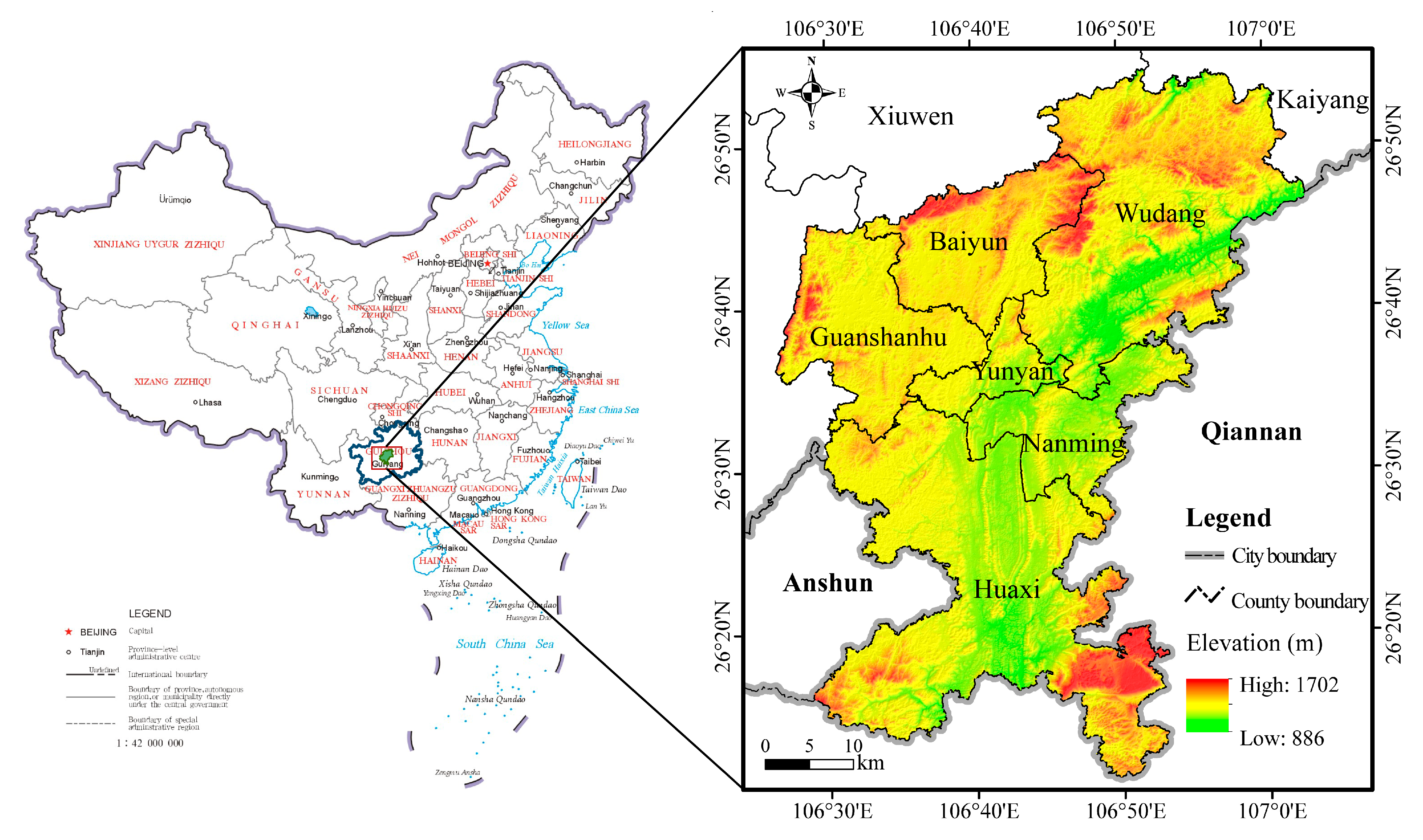
2.1. Study Area

Guiyang (106°26′–107°5′ E, 26°10′–26°55′ N) is a city situated in southwest China and the eastern slope of the Yunnan-Guizhou Plateau (Figure 1). It is composed of six districts: Yunyan, Nanming, Baiyun, Huaxi, Wudang, and Guanshanhu, covering a total area of 2525.46 km2 [22]. The terrain consists mainly of mountains, hills, and basins, with an average elevation of approximately 1100 m. Many karst formations occur across this area, and karst types are the most abundant in the world [23]. Dominated by a typical subtropical humid monsoon climate, this region has an average yearly temperature, precipitation, and relative humidity of 15.3 °C, 1197–1248 mm, and 77%, respectively [22]. The zonal soil type belongs to red and yellow soils that are formed under subtropical broadleaved forests, and the forest resources in this region are diverse [23]. Broadleaved forests and mixed conifer forests are the most broadly distributed vegetation types; evergreen scrub and subtropical scrub are also predominant after rapid urbanization and immense deforestation [24]. As one of the first batch of low-carbon pilot cities, Guiyang City has gained remarkable positive effects in carbon emission efficiency and forest management [22].

2.2. Data Collection and Processing

2.2.1. Carbon Storage and Carbon Density

The essence of the national forest resources inventory in China is to reset and measure the sample plots laid out by state and local governments, including land type, forest type, dominant tree species groups, stand origin, stock volume, stand age, and other information [25]. In this study, based on the fourth forest resources inventory database of Guizhou province in 2016, the regression relationships between the biomass and stand volume amount of different dominant species groups (Table 1) were established by adopting the method of a continuous function of dominant tree species and their biomass conversion factors [5]. The carbon storage of forest vegetation was calculated according to the formula based on the appropriate carbon content of forest vegetation of each species determined by referring to the literature data and the biomass of forest vegetation [26]. The carbon storage of forest vegetation was set as follows [26]:
A O C = i = 1 n A G B i × C i
where A O C is carbon storage of above-ground biomass (t); i are the forest type; n is the number of forest types; A G B i is the biomass of forest vegetation in the i -th forest type (t); and C i is the carbon content of forest vegetation in the i -th forest type (%).
The soil organic carbon storage of different forest types was calculated by using the average carbon content of main soil profile types of vegetation types in the soil census data of Guizhou province. The formula is shown as follows:
S O C = i , j = 1 n S i j × S C D j
where S O C is the soil organic carbon storage (t); i are the forest types; j are the soil types; n is the number of forest types; S i j is the area of j -th soil type in the i -th forest type (hm2); and S C D j is the organic carbon density of j -th soil type (t/hm2). The organic carbon density in each soil type was measured in 2005 [29].
Carbon density is calculated as the total carbon storage of the forest type divided by the forest area:
C D i = A O C i + S O C i S i
where C D i is the carbon density of the i -th forest type (t/hm2); A O C i and S O C i are the carbon storage of above-ground biomass and soil (t), respectively; and S i is the area of i -th forest type (hm2).

2.2.2. Site Conditions

The construction of the assessment index system should follow the basic principles, including comprehensiveness, accessibility, and feasibility. Based on the existing research results [11,30], 52 site factors were selected in this study, including the natural factors, socio-economic factors, and technological factors of Guiyang City (Table 2). Elevation data (DEM) with 30 resolutions were downloaded from the International Scientific and Technical Data website of the Chinese Academy of Sciences (http://www.gscloud.cn/ (accessed on 10 April 2022)), whereas slope, aspect, slope position, and terrain relief were derived from DEM using appropriate tools in ArcGIS 10.5 software (Environmental Systems Research Institute, Inc., Redlands, CA, USA). Construction density, vegetation coverage, and soil parent materials were extracted from the forest inventory data of Guizhou Province in 2016. The data of soil physical and chemical characteristics were obtained from China dataset of soil properties in 2013 [31]. Road network density and population density were downloaded from the open-access databases.

2.3. Spatial Autocorrelation Analysis

The spatial autocorrelation is used to reflect a geographical phenomenon on a regional unit or the degree of correlation between an attribute value and the same geographical phenomenon or attribute value on the adjacent unit, involving global spatial autocorrelation and local spatial autocorrelation [32]. In this study, spatial autocorrelation of forest ecosystem carbon density was analyzed using GeoDa 1.18 software (Luc Anselin. Chicago, IL, USA).
Global spatial autocorrelation is used to describe the overall distribution of a phenomenon and judge whether it has spatial correlation or spatial agglomeration [33]. Additionally, Moran’s I is commonly used as an indicator of global spatial autocorrelation. The formula is shown as follows [33]:
I = n i = 1 n j = 1 n w i j ( x i x ¯ ) ( x j x ¯ ) i = 1 n j = 1 n w i j ( i = 1 n ( x i x ¯ ) 2 )
where I is the Global Moran’s I ; w i j is the spatial weight matrix; x i and x j are the values of the attribute of cells i and j , respectively; and x ¯ is the average value of the attributes of all cells. The value range of Global Moran’s I is [−1, 1]. A value greater than 0 and less than 0 implies that the attribute distribution has positive and negative spatial autocorrelation, respectively. Zero value indicates no correlation, which is a random distribution.
Local spatial autocorrelation is used to decompose the global spatial autocorrelation into various spatial units and is normally specified by Anselin Local Moran’s I [33]. The values of Anselin Local Moran’s I can indicate clusters and outliers that represent positive and negative spatial autocorrelation, and can find out the regions that may be different from the global autocorrelation [34]. The formula is as follows [34]:
I i = x i x ¯ S 2 j w i j ( x j x ¯ )
where I i is the Anselin Local Moran’s I ; w i j is the spatial weight matrix; x i and x j are the standardized values of the attribute of cells i and j , respectively; and x ¯ is the average value of the attributes of all cells. The value of I i is [–1, 1]. It was divided into five types: High–high (H–H) clustering, Low–high (L–H) clustering, Low–low (L–L) clustering, High–low (H–L) clustering, and Not Significant.

2.4. Random Forest Model

The random forest model, proposed by Leo Breiman [35], is a parallel boosted machine learning algorithm which combines bagging and regression tree. It employs Bootstrap randomized re-sampling to repeatedly and randomly extract multiple versions of the sample sets from the original training datasets, then builds a decision tree model for each sample set; finally, combining all the results of the decision trees to predict the results of classification by the established voting mechanism [36]. This model has been widely used in ecological studies related to both classification and regression.
Based on the random forest package in R 4.1.2 (Ross Ihaka & Robert Gentleman. Auckland, NZ), 52 site factors affecting the spatial distribution pattern of forest carbon density were selected and the corresponding eigenvalue in each grid was calculated to construct the eigenmatrix, then the importance of site factors was judged according to the Mean-Decreased-Gini values [37]. In addition, about 70% of the dataset was used for model building (training) and the remaining 30% was used for model testing. The “optimal” model is determined by data division, cross validation, parameter tuning, and training complexity of the balance model. The out-of-bag error rate is also used to evaluate the model classification accuracy to avoid model overfitting [38].

2.5. Spatial Autoregression Model

Spatial autoregression models were used to investigate the factors affecting carbon density in this paper. The spatial autoregression model introduced spatial dependence into the ordinary least squares (OLS) regression, which considers the interaction of adjacent geographical units and aims to explain the dependent variables by a linear weighted combination of independent variables [39]. Both the spatial lag model and spatial error model are typical spatial regression models; however, there are still enough differences between them [40]. The OLS, SLM, and SEM can be defined as follows, respectively [41]:
O L S : Y = β X + ε S L M : Y = α 0 + ρ W Y + β X + ε S E M : { Y = α 0 + β X + μ μ = ( I λ W ) 1 ε
where β is the coefficients of driving factors X ; ε is a random error; W denotes the standardized spatial weight matrix; ρ denotes the coefficient of spatial lag; I denotes a unit vector; and λ denotes the coefficient of the spatial error.

3. Results

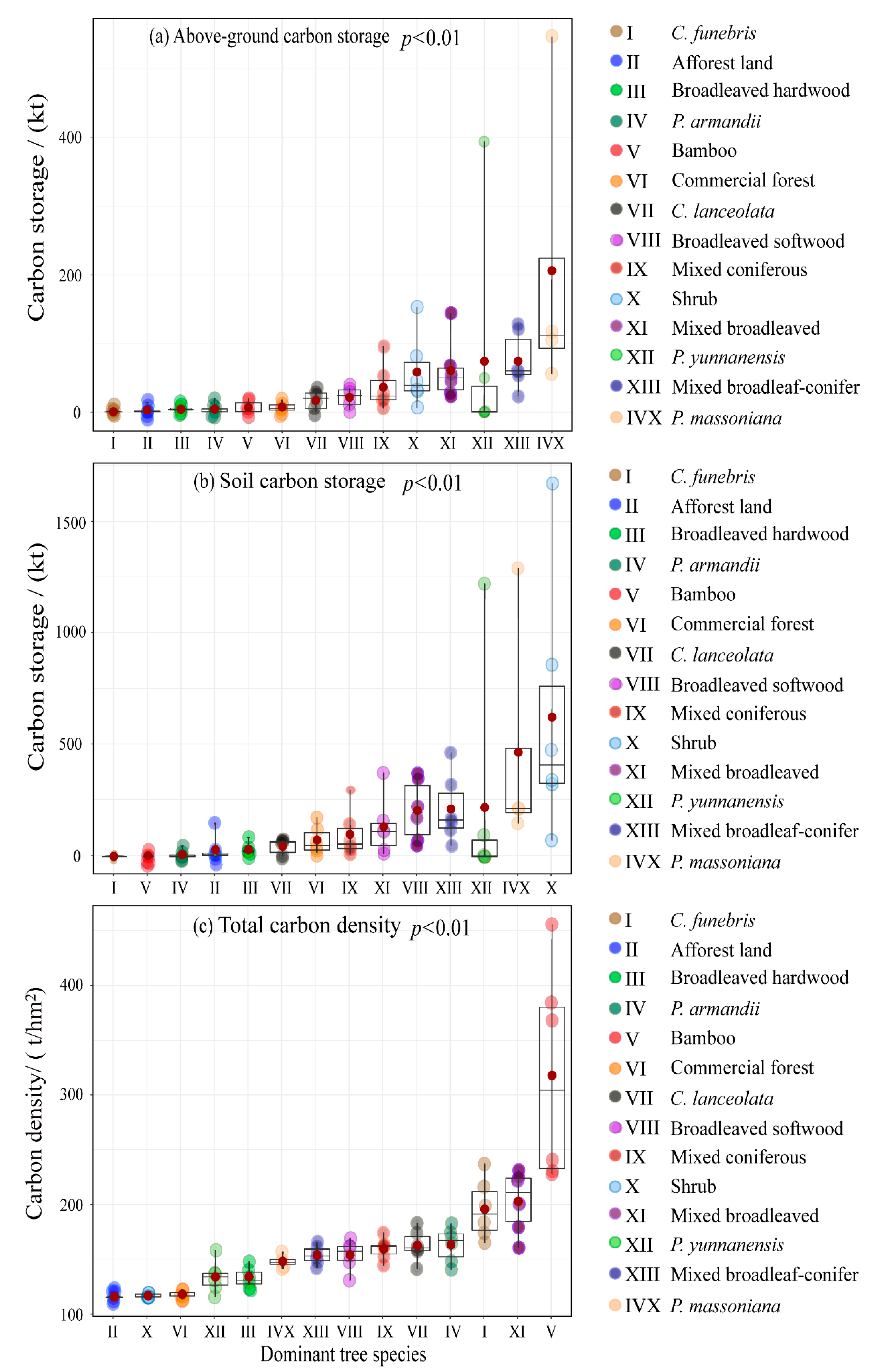
3.1. Carbon Density Assessment in Different Forest Types

The total carbon stock of the forest ecosystem was 15.25 × 10³ kt, with the average carbon density in fourteen major forests of 145.71 t/hm2. Among them, the above-ground carbon storage and soil carbon storage were 3.05 × 10³ kt and 12.20 × 10³ kt, respectively. The non-parametric test results indicated that the carbon sequestration between fourteen major forests ecosystems had an extremely significant difference (p < 0.01) (Figure 2). For the above-ground carbon stocks, the carbon stocks of P. massoniana forests were the highest forest type, which were 2–630 times higher than other forests. This was followed by mixed broadleaf-conifer forest, which accounted for about 14.65% of the total amount of above-ground carbon stocks. The soil carbon stock in various forest types ranged from 2.29 to 628.35 kt, among the soil carbon stock of shrubs and P. massoniana forests were comparatively higher than that of other forests, accounting for 30.88% and 26.27% of the total soil carbon storage, respectively. The carbon density of different forests ranged from 115.64 to 317.84 t/hm2, with bamboo forest, arbor forest, commercial forest, shrub, and afforest land in descending order. The carbon density of mixed broadleaved forests and C. funebris forests were over 190 t/hm2, whereas the afforest land had the lowest amount of carbon stocks per unit area, only 115.64 t/hm2.

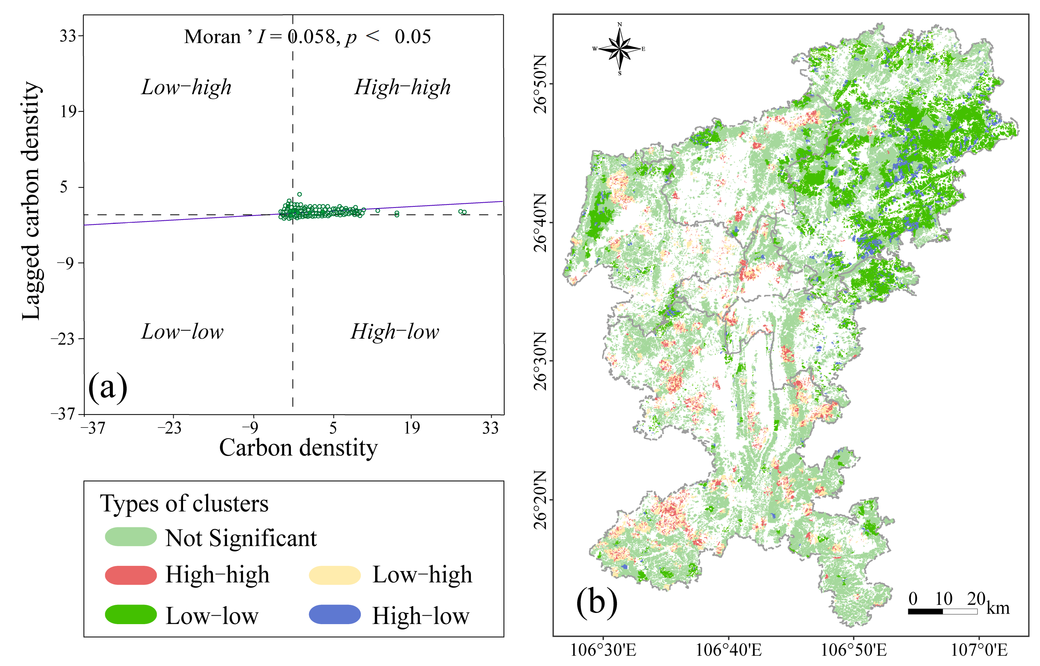
3.2. Spatial Heterogeneity of Carbon Density

The spatial distribution pattern of forest carbon density in the study area had significant spatial positive correlation and aggregation characteristics, with the global Moran’s I value of 0.058 (p < 0.05) (Figure 3a). A larger high–high clustering around the south-central part (Huaxi District) and the boundary between Yunyan District and Baiyun District of the study area were observed; negative spatial autocorrelation areas (Low–Low value clusters) were primarily concentrated in the north and northeast part of the study area; outlier areas were mostly located in the south or northwest (Figure 3b). Most of the high–low outliers (a high carbon density value in a low value region) were adjacent to the low–low clusters, as these areas had higher carbon density than the adjacent areas.

3.3. Relative Importance of Site Conditions on the Spatial Distribution of Carbon Density

The site conditions have a significant or highly significant negative or positive correlation with the spatial distribution of carbon density (Figure 4a). Across all 52 site conditions, the high–high cluster of carbon density was significantly negatively correlated with slope (F3), vegetation coverage (F9), terrain relief (F5), soil gravel content at 0 cm (F46), and slope position (F4). However, road density (F8), clay fraction at 16.6 cm (F19), and soil organic matter at 0–9.1 cm (F34, F35, F36) showed strong positive correlation with the high–high cluster of carbon density (p < 0.05). The soil gravel content at 0 cm (F46) had the largest negative driving effect (−0.05) on the low–low cluster of carbon density, whereas vegetation coverage (F9), soil parent material (F52), elevation (F2), road density (F8), the different layer thicknesses of sand fraction (F22–F27), and soil organic matter (F34–F39) were notably positively correlated with the low–low clustering areas of carbon density.
Random forest model analysis results indicated the carbon density in Guiyang City had a moderate spatial dependence, and the highest overall accuracy of the model was determined at twelve variables using tenfold hierarchical cross-validation (Figure 4b). The Mean-Decreased-Gini value was used to identify the top important variables affecting the spatial distribution of carbon density. The finding showed 0 cm cation exchange capacity (F10), soil parent material (F52), 9.1 cm silt fraction (F30), 28.9 cm soil organic matter (F38), road density (F8), cation exchange capacity at 4.5 cm (F11), and 9.1 cm soil pH (F42) were statistically significant at the 5% level. In addition, population density (F7), elevation (F2), slope (F3), construction density (F6), and vegetation coverage (F9) were not statistically significant at the 5% level, although these five factors had relatively higher Mean Decrease Gini values (Figure 4c). These indicated that soil properties and human interference were the most important controllers in carbon density prediction.

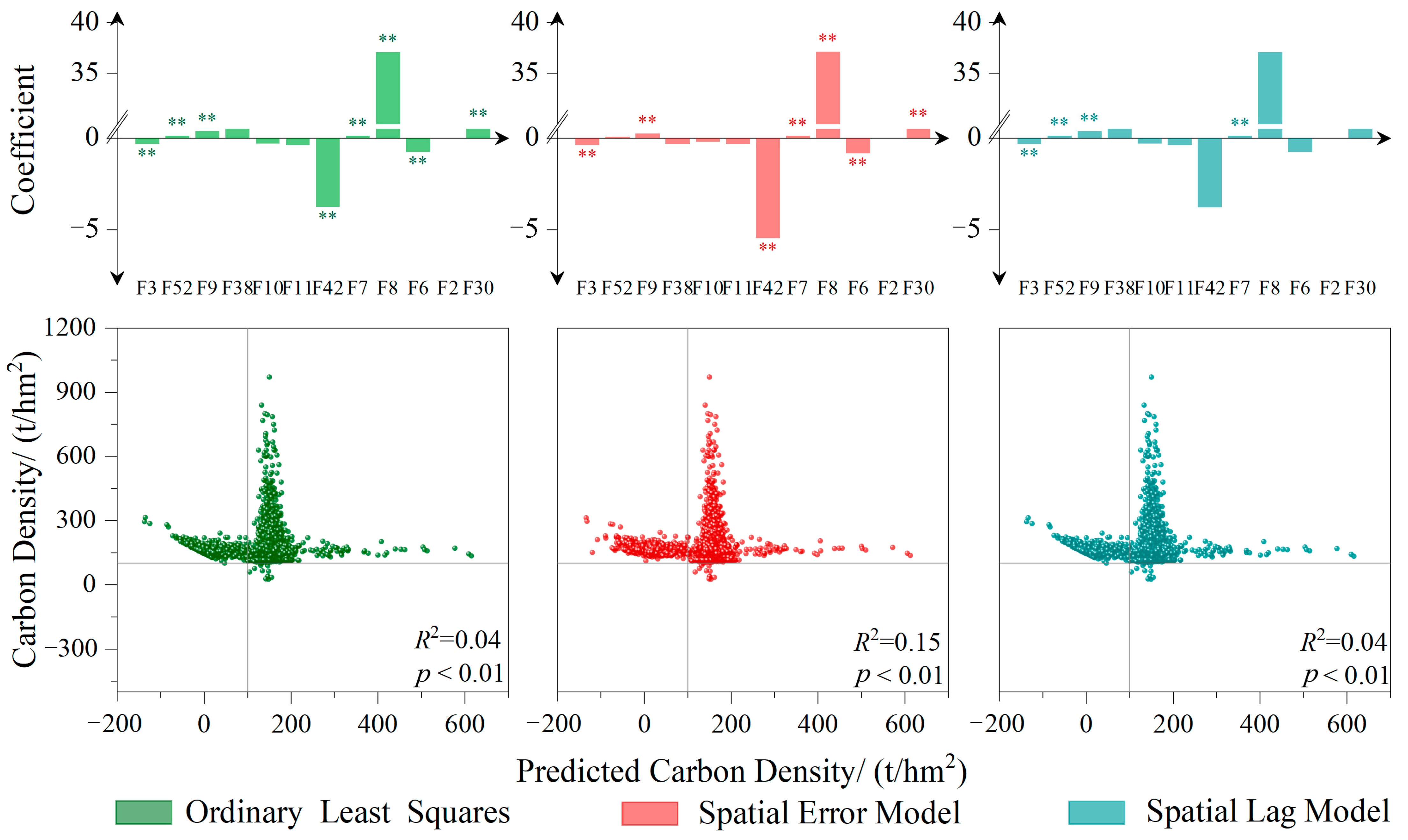
3.4. Driving Factors of the Spatial Differentiation on Carbon Density

Compared to the spatial regression results of OLS, SEM, and SLM, the SEM model with the largest coefficient of determination could better reflect the spatial heterogeneity of carbon density in the study area (Figure 5). The regression results of SEM model indicated that road density (F8) was the dominate positive influence factor of carbon density growth, followed by silt fraction at 9.1 cm (F30) and vegetation coverage (F9) (p < 0.01). Nevertheless, the carbon density was negatively influenced by the soil pH at 9.1 cm (F42), construction density (F6), and slope (F3) (p < 0.01).

4. Discussion

4.1. Urban Forest Carbon Sequestration Capacity

Forest carbon sequestration with a substantial carbon sink and high added value is considered to be the most promising way to mitigate global warming, and it is mainly affected by forest type, age of trees, climate, and human activities [42]. In this study, the average urban forest carbon density of vegetation pool and soil pool in Guiyang City was estimated at 145.71 t/hm2, which was lower than that in Gansu Province of China (279.51 t/hm2) during the same period and China national level (175.81 t/hm2) [43,44]. However, it was higher than the forest carbon density in Hunan Province (about 125 t/hm2) and other regions of Guizhou Province (85.94 t/hm2) [4,45]. The differences in forest carbon density among different regions might be attributed to a few possible reasons. On the one hand, forest types and forest age are pivotal factors in ecosystem carbon storage, and the proportion of young forests in the forest vegetation composition is inversely proportional to the accumulated biomass of the forest [42,46]. In the context of the rapid urbanization process, the serious overlogging of forests has led to a deterioration of forest ecosystem health. In order to restore the degradation of urban forest ecosystems, Guiyang City has implemented a series of ecological restoration programs since 2000, such as large-scale artificial planting and the establishment of forest protection zones [47]. However, the forest types in the study area were mainly secondary forests and the forest age mainly of young forests at present [25]. P. massoniana forests were the widely distributed in the study area, and their mature forest has the highest net primary productivity. Moreover, silvicultural species usually take a long time to become mature wood, resulting in a low stand volume per unit area. On the other hand, the carbon stock of forest ecosystem is influenced by the forest species composition and management patterns [48]. For example, the evidence provided by this study demonstrated that the carbon sequestration potential of bamboo forests was greater than that of other forests. Carbon sequestration per unit area of bamboo forests was 1–2 times higher than P. massoniana forests and C. lanceolata forests. This finding is consistent with previous related studies by Yen et al. [49]. However, bamboo forest was not a common and widely distributed forest ecosystem in the study area. Overall, inappropriate species composition, wide distribution of secondary young forests, and weak production per unit area led to differences in carbon storage and sequestration capacity of urban forests in the study area. Whereas urban forest productivity still has a significant amount of potential for enhancement, strengthening forest regeneration, improving the virtuous cycle ability of forest ecosystems, and optimizing forest structures might be effective strategies for enhancing the carbon sequestration ability of urban forests in the study area.

4.2. Response of Carbon Sequestration Ability to Site Conditions

The variabilities in carbon densities and their spatial distribution patterns are affected by natural and anthropogenic factors, especially in the ecologically sensitive and vulnerable regions with weak anti-interference ability and strong human activity interference [10,50]. As a typical karst fragile ecological area, the vulnerable background attribute of Guiyang City has changed the structure of plant communities and species diversity, which also affected soil formation and distribution [51]. In this study, the influence of site conditions on the carbon density of fourteen forest species concluded that the human disturbance and soil properties were responsible for the heterogeneity of carbon density (Figure 4), which is similar to the results of the study by Zald et al. in H.J. Andrews Experimental Forest [52]. Determinants that resulted in significant differences in carbon density included silt fraction at 9.1 cm, vegetation coverage, soil pH at 9.1 cm, slope, and urbanization level in this study. We discovered that the silt fraction at 9.1 cm and vegetation coverage had positive effects on carbon density. Soil pH at 9.1 cm had more impact on carbon density than vegetation coverage and slope. This proposed that vegetation would sequester more carbon in neutral or weakly acidic soils and on flat terrains. Furthermore, 0 cm cation exchange capacity and soil parent material were identified as the top predictors in shaping the spatial distribution patterns of forest carbon density, with the Mean-Decreased-Gini value of these two factors greater than 200 (Figure 4c). This agrees with the findings elsewhere [38,53], because cation exchange capacity (CEC) is a crucially reliable indicator of soil fertility, which has a strong positive correlation with the amount of organic matter in the soil [54]. From the perspective of community succession, soil parent material was one of the fundamental factors limiting or promoting carbon accumulation in terrestrial ecosystems [55]. However, soil erosion is more grievous in karst areas than in other regions, and soil loss causes ecosystem instability and productivity decline. Therefore, soil loss and low soil fertility had a negative effect on the carbon sequestration efficiency of forest in the study area.
Urbanization has significantly altered the carbon balance of ecosystems, and the conversion of landscapes from natural and agricultural to urbanized could have a direct or indirect effect on the carbon storage and regulation of urban ecosystems [56]. Construction density is one of the quantitative indicators of the level of urbanization [57]. In this study, construction density had an extremely significant negative correlation with the forest carbon density (Figure 5), which might be related to the influence of urbanization in the study area. The natural vegetation was replaced with impervious surfaces due to the loss of prime agricultural and woodland soil, which reduced biodiversity and accelerated the decomposition of organic matter [58]. Meanwhile, the subsoil had been incorporated with chemical materials during the construction process which destroyed the soil texture and reduced soil carbon storage [59]. Road density is another important indicator to measure the level of urbanization development [60]. In this study, forest carbon density was significantly positive with the road density (Figure 5), the main reasons being that roads in the study area were mostly built on the subsoil horizon of the convergent slopes or plains, which formed by the nutrient-rich topsoil of the eroding slopes and promoted the accumulation of above-ground biomass [61]; moreover, the increase in the bottom soil bulk density caused by artificial compaction could lead to the gradual growth of soil organic carbon density [56]. Therefore, it indicated that the natural and seminatural ecosystems were susceptible to shift from carbon sink to carbon source, whereas adaptation and compensation mechanism of urban forest carbon sequestration can be formed through the internal mechanism of forest self-regulation and ecological restoration in highly urbanized areas.

4.3. Limitations and Future Work

The age structure of forests has a direct effect on forest biomass [62]. Considering the relatively young age structure of the forests in Guiyang’s forests, the effect of age on the estimation of carbon sequestration will be more pronounced in the future. However, volume–biomass equations are frequently developed for universal age groups [5,62]. Thus, it is necessary to develop the volume–biomass equations for different forest types at different age groups to accurately assess forest carbon sequestration capacity and explore the response of regional forest ecosystem carbon density to site conditions. Moreover, more attention should be paid to optimizing forest management patterns and implementing reasonable harvesting strategies in order to improve the quality of the current forests, enhance biomass carbon sequestration, and mitigate global climate change.

5. Conclusions

The urban forest ecosystem in Guiyang City has a substantial potential for carbon sequestration, with an average carbon density of 145.71 t/hm2. Due to various factors, including site conditions and forest management, the carbon densities of forests showed large spatial heterogeneity. The cation exchange capacity at 0 cm and soil parent material turned out to be the most important factors leading to the distribution of forest carbon density, which was not uniform across geographical regions. In addition, the interaction of slope, road density, soil pH at 9.1 cm, construction density, silt fraction at 9.1 cm, and vegetation coverage were important factors for the significant differences in carbon sequestration capacity. Human interference was the main cause of the abnormal variation in carbon density, while poor forest vegetation growth and low soil fertility were also influential factors in reducing carbon density.

Author Contributions

Methodology, X.Z.; data curation, X.Z.; writing—original draft preparation, X.Z.; visualization, X.Z.; software, X.Z. and C.H.; validation, C.H.; investigation, C.H.; writing—review and editing, Z.W.; supervision Z.W. All authors have read and agreed to the published version of the manuscript.

Funding

This research was funded by the National Nature Science Foundation of China (NSFC) project (Grant numbers 42061039 and 41701319), the Cultivation Project of Guizhou University, grant number (2020)46, and the Construction Program of Biology First-class Discipline in Guizhou, grant number GNYL (2017)009.

Institutional Review Board Statement

Not applicable.

Informed Consent Statement

Not applicable.

Data Availability Statement

Not applicable.

Acknowledgments

Authors are thankful to reviewers and editors for their insightful comments and suggestions to an earlier edition of this article.

Conflicts of Interest

The authors declare no conflict of interest.

References

  1. Gogoi, A.; Ahirwal, J.; Sahoo, U.K. Evaluation of ecosystem carbon storage in major forest types of Eastern Himalaya: Implications for carbon sink management. J. Environ. Manag. 2022, 302, 113972. [Google Scholar] [CrossRef] [PubMed]
  2. He, N.; Wen, D.; Zhu, J.; Tang, X.; Xu, L.; Zhang, L.; Hu, H.; Huang, M.; Yu, G. Vegetation carbon sequestration in Chinese forests from 2010 to 2050. Glob. Chang. Biol. 2017, 23, 1575–1584. [Google Scholar] [CrossRef] [PubMed]
  3. Sun, L.; Wang, Q.; Fan, X. An Integrative Approach to Study How Driving Factors Control Biomass Carbon Density for Natural Mountain Forests, in China’s Loess Plateau. Forests 2022, 13, 1114. [Google Scholar] [CrossRef]
  4. Chen, L.C.; Guan, X.; Li, H.M.; Wang, Q.K.; Zhang, W.D.; Yang, Q.P.; Wang, S.L. Spatiotemporal patterns of carbon storage in forest ecosystems in Hunan Province, China. For. Ecol. Manag. 2019, 432, 656–666. [Google Scholar] [CrossRef]
  5. Fang, J.; Chen, A.; Peng, C.; Zhao, S.; Ci, L. Changes in forest biomass carbon storage in China between 1949 and 1998. Science 2001, 292, 2320–2322. [Google Scholar] [CrossRef] [PubMed]
  6. Yang, J.; Ji, X.; Deane, D.C.; Wu, L.; Chen, S. Spatiotemporal distribution and driving factors of forest biomass carbon storage in China: 1977–2013. Forests 2017, 8, 263. [Google Scholar] [CrossRef]
  7. Li, X.; OuYang, X.; Liu, Q. Carbon storage of forest v.vegetation and its geographical pattern in China’s Jiangxi Province during 2001–2005. J. Nat. Resour. 2011, 26, 655–665. [Google Scholar] [CrossRef]
  8. Zhang, L.J.; Lai, G.H.; Zeng, W.S.; Zou, W.T.; Yi, S.J. Effect of Climate on Carbon Storage Growth Models for Three Major Coniferous Plantations in China Based on National Forest Inventory Data. Forests 2022, 13, 882. [Google Scholar] [CrossRef]
  9. Skovsgaard, J.P.; Vanclay, J.K. Forest site productivity: A review of spatial and temporal variability in natural site conditions. Forestry 2013, 86, 305–315. [Google Scholar] [CrossRef]
  10. Nave, L.E.; DeLyser, K.; Domke, G.M.; Holub, S.M.; Janowiak, M.K.; Kittler, B.; Ontl, T.A.; Sprague, E.; Sucre, E.B.; Walters, B.F.; et al. Disturbance and management effects on forest soil organic carbon stocks in the Pacific Northwest. Ecol. Appl. 2022, 32, e2611. [Google Scholar] [CrossRef]
  11. Huang, J.; Ge, Z.; Huang, Y.; Tang, X.; Shi, Z.; Lai, P.; Song, Z.; Hao, B.; Yang, H.; Ma, M. Climate change and ecological engineering jointly induced vegetation greening in global karst regions from 2001 to 2020. Plant Soil 2022, 475, 193–212. [Google Scholar] [CrossRef]
  12. Zhang, C.S.; Deng, Q.H.; Liu, A.B.; Liu, C.L.; Xie, G.D. Effects of Stand Structure and Topography on Forest Vegetation Carbon Density in Jiangxi Province. Forests 2021, 12, 1483. [Google Scholar] [CrossRef]
  13. Shi, W.Y.; Chen, Y.Z.; Feng, X.M. Identifying the terrestrial carbon benefits from ecosystem restoration in ecologically fragile regions. Agric. Ecosyst. Environ. 2020, 296, 106889. [Google Scholar] [CrossRef]
  14. Peng, T.; Deng, H. Research on the sustainable development process of low-carbon pilot cities: The case study of Guiyang, a low-carbon pilot city in south-west China. Environ. Dev. Sustain. 2021, 23, 2382–2403. [Google Scholar] [CrossRef]
  15. Liu, L.; Zeng, F.P.; Song, T.Q.; Wang, K.L.; Du, H. Stand Structure and Abiotic Factors Modulate Karst Forest Biomass in Southwest China. Forests 2020, 11, 443. [Google Scholar] [CrossRef]
  16. Zhou, B.; Liao, Z.; Chen, S.; Jia, H.; Zhu, J.; Fei, X. Net Primary Productivity of Forest Ecosystems in the Southwest Karst Region from the Perspective of Carbon Neutralization. Forests 2022, 13, 1367. [Google Scholar] [CrossRef]
  17. Zhang, C.; Zeng, F.; Zeng, Z.; Du, H.; Su, L.; Zhang, L.; Lu, M.; Zhang, H. Impact of Selected Environmental Factors on Variation in Leaf and Branch Traits on Endangered Karst Woody Plants of Southwest China. Forests 2022, 13, 1080. [Google Scholar] [CrossRef]
  18. Jiang, Y.; Meng, T.; Xu, W.; Tan, W.; Zhang, Q.; Liu, Y. Community characteristics of endangered Gymnosperms and their topographic relationships in a karst mountaintop region. Acta Ecol. Sin. 2021, 41, 1868–1877. [Google Scholar] [CrossRef]
  19. Song, X.W.; Gao, Y.; Wen, X.F.; Guo, D.L.; Yu, G.R.; He, N.P.; Zhang, J.Z. Carbon sequestration potential and its eco-service function in the karst area, China. J. Geogr. Sci. 2017, 27, 967–980. [Google Scholar] [CrossRef]
  20. Zhou, B.; Wang, G.; Tang, Y.; Zhang, W.; Zang, R. Zoning of degraded natural forests in mountain areas of Southwest China. For. Res. Beijing 2010, 23, 612–616. [Google Scholar]
  21. Liu, L.; Xiong, K.; Luo, Y. Advances in evaluation of sustainable development capability in karst region. Guizhou Agric. Sci. 2012, 41, 67–72. [Google Scholar] [CrossRef]
  22. Liu, Y.; Huang, X.; Yang, H.; Zhong, T. Environmental effects of land-use/cover change caused by urbanization and policies in Southwest China Karst area–A case study of Guiyang. Habitat Int. 2014, 44, 339–348. [Google Scholar] [CrossRef]
  23. Mingjun, L.; Lifei, Y.; Huanbai, X.; Chaojun, N.; Zongsheng, H.; Du Mingfeng, Z.; Jianhua, S. The Prediction of Forest Carbon Sequestration Dynamics in Guizhou Province and Relevant Influencing Factors. Pak. J. Bot. 2018, 50, 1157–1170. [Google Scholar] [CrossRef]
  24. Yang, J.; Luo, X.; Lu, S.; Yang, Y.; Yang, J. Effects of compositional and configurational heterogeneity of the urban matrix on the species richness of woody plants in urban remnant forest patches. Landsc. Ecol. 2022, 37, 619–632. [Google Scholar] [CrossRef]
  25. Lu, J.; Feng, Z.K.; Zhu, Y. Estimation of Forest Biomass and Carbon Storage in China Based on Forest Resources Inventory Data. Forests 2019, 10, 650. [Google Scholar] [CrossRef]
  26. Li, M.; Du, M.; Yu, L. Carbon storage and density of forest vegetation and its spatial distribution pattern in Guizhou Province. J. Northwest. For. Univ. 2016, 31, 48–54. [Google Scholar] [CrossRef]
  27. Tian, X.L.; Xia, J.; Xia, H.B.; Ni, J. Forest biomass an.nd its spatial pattern in Guizhou Province. Chin. J. Appl. Ecol. 2011, 22, 287–294. [Google Scholar]
  28. Zhou, J.; Xu, S. Analysis of the current status and dynamics of forest carbon storage in Yunnan Province. For. Invent. Plan. 2016, 41, 17–23. [Google Scholar]
  29. Yu, D.; Shi, X.; Sun, W.; Wang, H.; Liu, Q.; Zhao, Y. Estimation of China soil organic carbon storage and density based on 1: 1,000,000 soil database. Chin. J. Appl. Ecol. 2005, 16, 2279–2283. [Google Scholar]
  30. Bedane, G.A.; Feyisa, G.L.; Senbeta, F. Spatial distribution of above ground carbon density in Harana Forest, Ethiopia. Ecol. Process. 2022, 11, 1–13. [Google Scholar] [CrossRef]
  31. Shangguan, W.; Dai, Y.; Liu, B.; Zhu, A.; Duan, Q.; Wu, L.; Ji, D.; Ye, A.; Yuan, H.; Zhang, Q. A China data set of soil properties for land surface modeling. J. Adv. Model. Earth Syst. 2013, 5, 212–224. [Google Scholar] [CrossRef]
  32. Cui, Y.; Li, L.; Chen, L.; Zhang, Y.; Cheng, L.; Zhou, X.; Yang, X. Land-use carbon emissions estimation for the Yangtze River Delta Urban Agglomeration using 1994–2016 Landsat image data. Remote Sens. 2018, 10, 1334. [Google Scholar] [CrossRef]
  33. Hu, X.; Ma, C.; Huang, P.; Guo, X. Ecological vulnerability assessment based on AHP-PSR method and analysis of its single parameter sensitivity and spatial autocorrelation for ecological protection–A case of Weifang City, China. Ecol. Indic. 2021, 125, 107464. [Google Scholar] [CrossRef]
  34. Li, W.; Dong, F.; Ji, Z. Research on coordination level and influencing factors spatial heterogeneity of China’s urban CO2 emissions. Sustain. Cities Soc. 2021, 75, 103323. [Google Scholar] [CrossRef]
  35. Breiman, L. Bagging predictors. Mach. Learn. 1996, 24, 123–140. [Google Scholar] [CrossRef]
  36. Fang, X.; Li, X.; Zhang, Y.; Zhao, Y.; Qian, J.; Hao, C.; Zhou, J.; Wu, Y. Random forest-based understanding and predicting of the impacts of anthropogenic nutrient inputs on the water quality of a tropical lagoon. Environ. Res. Lett. 2021, 16, 055003. [Google Scholar] [CrossRef]
  37. Han, H.; Guo, X.; Yu, H. Variable selection using mean decrease accuracy and mean decrease gini based on random forest. In Proceedings of the 2016 7th IEEE International Conference on Software Engineering and Service Science (Icsess), Beijing, China, 26–28 August 2016; IEEE: New York, NY, USA, 2016; pp. 219–224. [Google Scholar]
  38. Zhang, L.; Huettmann, F.; Zhang, X.; Liu, S.; Sun, P.; Yu, Z.; Mi, C. The use of classification and regression algorithms using the random forests method with presence-only data to model species’ distribution. MethodsX 2019, 6, 2281–2292. [Google Scholar] [CrossRef]
  39. Guo, J.; Han, G.; Xie, Y.; Cai, Z.; Zhao, Y. Exploring the relationships between urban spatial form factors and land surface temperature in mountainous area: A case study in Chongqing city, China. Sustain. Cities Soc. 2020, 61, 102286. [Google Scholar] [CrossRef]
  40. Conway, D.; Li, C.Q.; Wolch, J.; Kahle, C.; Jerrett, M. A spatial autocorrelation approach for examining the effects of urban greenspace on residential property values. J. Real Estate Financ. Econ. 2010, 41, 150–169. [Google Scholar] [CrossRef]
  41. Gu, Y.L.; You, X.Y. A spatial quantile regression model for driving mechanism of urban heat island by considering the spatial dependence and heterogeneity: An example of Beijing, China. Sustain. Cities Soc. 2022, 79, 103692. [Google Scholar] [CrossRef]
  42. Lorenz, K.; Lal, R. Carbon Sequestration in Forest Ecosystems; Springer: Berlin/Heidelberg, Germany, 2009; pp. 103–146. [Google Scholar]
  43. Guan, J.; Du, S.; Cheng, J.; Wu, C.; Li, G.; Deng, L.; Zhang, J.; He, Q.; Shi, W. Current stocks and rate of sequestration of forest carbon in Gansu Province, China. Chin. J. Plant Ecol. 2016, 40, 304. [Google Scholar] [CrossRef]
  44. Sun, W.; Liu, X. Review on carbon storage estimation of forest ecosystem and applications in China. For. Ecosyst. 2020, 7, 1–14. [Google Scholar] [CrossRef]
  45. Guo, C.; Wu, Y.; Ni, J.; Guo, Y. Forest carbon storage in Guizhou Province based on field measurement dataset. Acta Geochim. 2019, 38, 8–21. [Google Scholar] [CrossRef]
  46. Wei, Y.; Li, M.; Chen, H.; Lewis, B.J.; Yu, D.; Zhou, L.; Zhou, W.; Fang, X.; Zhao, W.; Dai, L. Variation in carbon storage and its distribution by stand age and forest type in boreal and temperate forests in northeastern China. PLoS ONE 2013, 8, e72201. [Google Scholar] [CrossRef] [PubMed] [Green Version]
  47. Tang, Y.; Shao, Q.; Shi, T.; Lu, Z.; Wu, G. Spatiotemporal dynamics of forest ecosystem carbon budget in Guizhou: Customisation and application of the CBM-CFS3 model for China. Carbon Balance Manag. 2022, 17, 1–24. [Google Scholar] [CrossRef] [PubMed]
  48. Xiang, M.; Wang, C.; Tan, Y.; Yang, J.; Duan, L.; Fang, Y.; Li, W.; Shu, Y.; Liu, M. Spatio-temporal evolution and driving factors of carbon storage in the Western Sichuan Plateau. Sci. Rep. 2022, 12, 8114. [Google Scholar] [CrossRef]
  49. Yen, T.-M.; Lee, J.-S. Comparing aboveground carbon sequestration between moso bamboo (Phyllostachys heterocycla) and China fir (Cunninghamia lanceolata) forests based on the allometric model. For. Ecol. Manag. 2011, 261, 995–1002. [Google Scholar] [CrossRef]
  50. Sun, L.N.; Wang, M.B.; Fan, X.H. Spatial pattern and driving factors of biomass carbon density for natural and planted coniferous forests in mountainous terrain, eastern Loess Plateau of China. For. Ecosyst. 2020, 7, 1–13. [Google Scholar] [CrossRef]
  51. Liu, F.; Wu, H.Y.; Zhao, Y.G.; Li, D.C.; Yang, J.L.; Song, X.D.; Shi, Z.; Zhu, A.X.; Zhang, G.L. Mapping high resolution National Soil Information Grids of China. Sci. Bull. 2022, 67, 328–340. [Google Scholar] [CrossRef]
  52. Zald, H.S.; Spies, T.A.; Seidl, R.; Pabst, R.J.; Olsen, K.A.; Steel, E.A. Complex mountain terrain and disturbance history drive variation in forest aboveground live carbon density in the western Oregon Cascades, USA. For. Ecol. Manag. 2016, 366, 193–207. [Google Scholar] [CrossRef]
  53. Olorunfemi, I.E.; Fasinmirin, J.T.; Akinola, F.F. Soil physico-chemical properties and fertility status of long-term land use and cover changes: A case study in forest vegetative zone of Nigeria. Eurasian J. Soil Sci. 2018, 7, 133–150. [Google Scholar] [CrossRef]
  54. Fasinmirin, J.; Olorunfemi, I. Comparison of hydraulic conductivity of soils of the forest vegetative zone of Nigeria. Appl. Trop. Agric. 2012, 17, 64–77. [Google Scholar]
  55. Wiesmeier, M.; Urbanski, L.; Hobley, E.; Lang, B.; von Lützow, M.; Marin-Spiotta, E.; van Wesemael, B.; Rabot, E.; Ließ, M.; Garcia-Franco, N. Soil organic carbon storage as a key function of soils-A review of drivers and indicators at various scales. Geoderma 2019, 333, 149–162. [Google Scholar] [CrossRef]
  56. Liu, R.; Wang, M.; Chen, W. The influence of urbanization on organic carbon sequestration and cycling in soils of Beijing. Landsc. Urban Plan. 2018, 169, 241–249. [Google Scholar] [CrossRef]
  57. Liu, X.; Li, T.; Zhang, S.; Jia, Y.; Li, Y.; Xu, X. The role of land use, construction and road on terrestrial carbon stocks in a newly urbanized area of western Chengdu, China. Landsc. Urban Plan. 2016, 147, 88–95. [Google Scholar] [CrossRef]
  58. Ding, Z.; Zheng, H.; Li, H.; Yu, P.J.; Man, W.D.; Liu, M.Y.; Tang, X.G.; Liu, Y. Afforestation-driven increases in terrestrial gross primary productivity are partly offset by urban expansion in Southwest China. Ecol. Indic. 2021, 127, 107641. [Google Scholar] [CrossRef]
  59. Lorenz, K.; Lal, R. Carbon storage in some urban forest soils of Columbus, Ohio, USA. In Carbon Sequestration in Urban Ecosystems; Springer: Dordrecht, Netherlands, 2012; pp. 139–158. [Google Scholar]
  60. Zhu, Z.P.; Li, J.Y.; Chen, Z.R. Green space equity: Spatial distribution of urban green spaces and correlation with urbanization in Xiamen, China. Environ. Dev. Sustain. 2022, 24, 1–21. [Google Scholar] [CrossRef]
  61. Berhe, A.A.; Harte, J.; Harden, J.W.; Torn, M.S. The significance of the erosion-induced terrestrial carbon sink. BioScience 2007, 57, 337–346. [Google Scholar] [CrossRef]
  62. Pan, Y.; Luo, T.; Birdsey, R.; Hom, J.; Melillo, J. New estimates of carbon storage and sequestration in China’s forests: Effects of age–class and method on inventory-based carbon estimation. Clim. Change 2004, 67, 211–236. [Google Scholar] [CrossRef]
Figure 1. Location of the study site.
Forests 13 01484 g001
Figure 2. The carbon storages of above-ground biomass in different forest types (a); the carbon storages of soil in different forest types (b); the total carbon densities in different forest types (c).
Forests 13 01484 g002
Figure 3. The Moran scatter diagram of carbon density (a); cluster map of carbon density detected by Anselin Local Moran’s I (b).
Forests 13 01484 g003
Figure 4. Spearman correlation between locations of the carbon density clustering and each site condition (a); strengths of site conditions of model variables based on Gini values (b,c). ** indicates significant differences at p < 0.01 (Significant test).
Forests 13 01484 g004
Figure 5. The parameter estimation results of the least square model, spatial error model, and spatial lag model. ** indicates significant differences at p < 0.01 (Significant test).
Forests 13 01484 g005
Table 1. Volume–biomass equations and carbon concentration of dominant tree species.
Dominant Tree Species (Group)Volume–Biomass EquationsCarbon Content/%Reference
Afforest land A G B = 19.76 S 50.00[27]
Bamboo A G B = 22.5 N / 1000 46.69[5]
Broadleaved hardwood A G B = 1.0357 x + 8.0591 49.34[27]
Broadleaved softwood A G B = 0.4750 x + 30.6030 49.56[28]
Commercial forest A G B = 23.70 S 45.51[5]
Cunninghamia lanceolata (Lamb.) Hook. A G B = 0.3999 x + 22.5410 55.28[5]
Cupressus funebris Endl. A G B = 0.6129 x + 46.1451 51.00[5]
Mixed broadleaf-conifer A G B = 0.8019 x + 12.2799 49.78[5]
Mixed broadleaved A G B = 0.6255 x + 91.0013 49.00[5]
Mixed conifer A G B = 0.5894 x + 24.5151 51.00[5]
Pinus armandii Franch. A G B = 0.5856 x + 18.7435 52.25[5]
Pinus massoniana Lamb. A G B = 0.5101 x + 1.0451 59.84[5]
Pinus yunnanensis Franch. A G B = 0.5101 x + 1.0451 51.13[5]
Shrub A G B = 19.76 S 50.47[5]
Note: AGB, above-ground biomass; x (t), timber volume per unit area (m3/hm2); S , area of forests (hm2); N , number of bamboo stems; Carbon content, the percentage of organic carbon in the total mass of plant organic matter (%).
Table 2. List of forest site conditions.
Stand IndicatorsShort NameResolutionData Sources
AspectF130 mhttp://www.gscloud.cn/
(accessed on 10 April 2022)
Elevation (m)F230 mhttp://www.gscloud.cn/
(accessed on 10 April 2022)
Slope (°)F330 mhttp://www.gscloud.cn/
(accessed on 10 April 2022)
Slope positionF430 mhttp://www.gscloud.cn/
(accessed on 10 April 2022)
Terrain relief (°)F530 mhttp://www.gscloud.cn/
(accessed on 10 April 2022)
Construction density (m2/hectare) F630 mForest inventory data
Population density (people/hectare)F7100 mhttps://www.worldpop.org/
(accessed on 28 April 2022)
Road network density (m/hectare)F830 mhttps://www.openstreetmap.org/
(accessed on 28 April 2022)
Vegetation coverage (%)F930 mForest inventory data
Cation exchange capacity at 0 cm (me/100 g)F1030 arc-secondNational Tibetan Plateau Data Center
Cation exchange capacity at 4.5 cm (me/100 g)F1130 arc-secondNational Tibetan Plateau Data Center
Cation exchange capacity at 9.1 cm (me/100 g)F1230 arc-secondNational Tibetan Plateau Data Center
Cation exchange capacity at 16.6 cm (me/100 g)F1330 arc-secondNational Tibetan Plateau Data Center
Cation exchange capacity at 28.9 cm (me/100 g)F1430 arc-secondNational Tibetan Plateau Data Center
Cation exchange capacity at 49.3 cm (me/100 g)F1530 arc-secondNational Tibetan Plateau Data Center
Clay fraction at 0 cm (%)F1630 arc-secondNational Tibetan Plateau Data Center
Clay fraction at 4.5 cm (%)F1730 arc-secondNational Tibetan Plateau Data Center
Clay fraction at 9.1 cm (%)F1830 arc-secondNational Tibetan Plateau Data Center
Clay fraction at 16.6 cm (%)F1930 arc-secondNational Tibetan Plateau Data Center
Clay fraction at 28.9 cm (%)F2030 arc-secondNational Tibetan Plateau Data Center
Clay fraction at 49.3 cm (%)F2130 arc-secondNational Tibetan Plateau Data Center
Sand fraction at 0 cm (%)F2230 arc-secondNational Tibetan Plateau Data Center
Sand fraction at 4.5 cm (%)F2330 arc-secondNational Tibetan Plateau Data Center
Sand fraction at 9.1 cm (%)F2430 arc-secondNational Tibetan Plateau Data Center
Sand fraction at 16.6 cm (%)F2530 arc-secondNational Tibetan Plateau Data Center
Sand fraction at 28.9 cm (%)F2630 arc-secondNational Tibetan Plateau Data Center
Sand fraction at 49.3 cm (%)F2730 arc-secondNational Tibetan Plateau Data Center
Silt fraction at 0 cm (%)F2830 arc-secondNational Tibetan Plateau Data Center
Silt fraction at 4.5 cm (%)F2930 arc-secondNational Tibetan Plateau Data Center
Silt fraction at 9.1 cm (%)F3030 arc-secondNational Tibetan Plateau Data Center
Silt fraction at 16.6 cm (%)F3130 arc-secondNational Tibetan Plateau Data Center
Silt fraction at 28.9 cm (%)F3230 arc-secondNational Tibetan Plateau Data Center
Silt fraction at 49.3 cm (%)F3330 arc-secondNational Tibetan Plateau Data Center
Soil organic matter at 0 cm (%)F3430 arc-secondNational Tibetan Plateau Data Center
Soil organic matter at 4.5 cm (%)F3530 arc-secondNational Tibetan Plateau Data Center
Soil organic matter at 9.1 cm (%)F3630 arc-secondNational Tibetan Plateau Data Center
Soil organic matter at 16.6 cm (%)F3730 arc-secondNational Tibetan Plateau Data Center
Soil organic matter at 28.9 cm (%)F3830 arc-secondNational Tibetan Plateau Data Center
Soil organic matter at 49.3 cm (%)F3930 arc-secondNational Tibetan Plateau Data Center
Soil pH at 0 cmF4030 arc-secondNational Tibetan Plateau Data Center
Soil pH at 4.5 cmF4130 arc-secondNational Tibetan Plateau Data Center
Soil pH at 9.1 cmF4230 arc-secondNational Tibetan Plateau Data Center
Soil pH at 16.6 cmF4330 arc-secondNational Tibetan Plateau Data Center
Soil pH at 28.9 cmF4430 arc-secondNational Tibetan Plateau Data Center
Soil pH at 49.3 cmF4530 arc-secondNational Tibetan Plateau Data Center
Soil gravel content at 0 cm (%)F4630 arc-secondNational Tibetan Plateau Data Center
Soil gravel content at 4.5 cm (%)F4730 arc-secondNational Tibetan Plateau Data Center
Soil gravel content at 9.1 cm (%)F4830 arc-secondNational Tibetan Plateau Data Center
Soil gravel content at 16.6 cm (%)F4930 arc-secondNational Tibetan Plateau Data Center
Soil gravel content at 28.9 cm (%)F5030 arc-secondNational Tibetan Plateau Data Center
Soil gravel content at 49.3 cm (%)F5130 arc-secondNational Tibetan Plateau Data Center
Soil parent materialsF5230 mForest inventory data
Publisher’s Note: MDPI stays neutral with regard to jurisdictional claims in published maps and institutional affiliations.

