Abstract
Unmanned aerial systems (UASs) and structure-from-motion (SfM) image processing are promising tools for sustainable forest management as they allow for the generation of photogrammetrically derived point clouds from UAS images that can be used to estimate forest structure, for a fraction of the cost of LiDAR. The SfM process and the quality of products produced, however, are sensitive to the chosen flight parameters. An understanding of the effect flight parameter choice has on accuracy will improve the operational feasibility of UASs in forestry. This study investigated the change in the plot-level accuracy of top-of-canopy height (TCH) across three levels of flying height (80 m, 100 m, and 120 m) and four levels of forward overlap (80%, 85%, 90%, and 95%). A SenseFly eBee X with an Aeria X DSLR camera was used to collect the UAS imagery which was then run through the SfM process to derive photogrammetric point clouds. Estimates of TCH were extracted for all combinations of flying height and forward overlap and compared to TCH estimated from ground data. A generalized linear model was used to statistically assess the effect of parameter choice on accuracy. The RMSE (root-mean-square error) of the TCH estimates (RMSETCH) ranged between 1.75 m (RMSETCH % = 5.94%) and 3.20m (RMSETCH % = 10.1%) across all missions. Flying height was found to have no significant effect on RMSETCH, while increasing forward overlap was found to significantly decrease the RMSETCH; however, the estimated decrease was minor at 4 mm per 1% increase in forward overlap. The results of this study suggest users can fly higher and with lower levels of overlap without sacrificing accuracy, which can have substantial time-saving benefits both in the field collecting the data and in the office processing the data.
1. Introduction
Forests provide numerous environmental services as well as contribute significantly to the local and global economy [1,2,3,4]. A long-term challenge associated with forest management is doing so in a sustainable manner, so that the current needs are met while maintaining healthy forest ecosystems for present and future generations [5,6]. To accomplish this goal, managers require spatially detailed, accurate, and timely information on a wide variety of forest structural metrics (e.g., quality and quantity of forest resources) to support operational and strategic planning and monitoring [6,7,8]. Timeliness and the type of data collected become even more important in the face of unpredictable changes to forest structure due to biotic and abiotic factors [9,10]. This task is difficult to achieve with traditional, ground-based, forest inventory. Traditional inventory is labor-intensive, especially for remote areas, time-consuming, and increasingly expensive to carry out. [6,11]. As a result, inventories typically cover small areas and limit the number and types of measurements made on the ground [6,9].
Remote sensing has offered an efficient and effective opportunity to study and quantify ecological phenomena over broader spatial and temporal scales than fieldwork alone for some time now [12,13,14]. In the forestry community, remotely sensed data have been an invaluable tool to expand the spatial, temporal, and dimensional extent of their data collection, allowing managers to better develop and implement sustainable management strategies [6,8,15,16]. LiDAR remote sensing has long been the popular source of information for structural estimates, given its ability to sample vegetation within the canopy. Therefore, LiDAR provides information on both horizontal and vertical vegetation distributions; optical sensors (i.e., imagery) have traditionally provided only horizontal information [17]. Various descriptive variables believed to relate to the forest structure are extracted from the LiDAR data and used as the explanatory variable in models predicting the structural variable of interest (e.g., canopy cover, basal area, volume, above ground biomass, height) [18,19,20,21]. Ground samples collected by traditional forest inventory or other sources act as the training/validation. Using the developed model, the remainder of the nonsampled areas are estimated to create a wall-to-wall map of that metric [22,23,24,25,26].
In general, the process of converting LiDAR data into reliable estimates of structure is well understood [22,27,28]; however, the high cost of the data continues to limit its operational feasibility, especially if repeat collection in a narrow time frame is necessary [8,9]. Recent technological advancements have led to a potential solution. Unmanned aerial systems (UASs) have become a reliable and affordable platform for collecting remotely sensed data. UASs offer several advantages over traditional platforms such as satellite or manned aircraft [14]. Satellite remotely sensed data are very appealing because the extent of the data can be regional to global in scale and many satellites have repeat collections [29]. However, given their distance from the earth’s surface, many data do not have spatial or temporal resolutions that are appropriate for many fine-scale ecological phenomena. Data from commercial satellites that offer higher spatial resolutions are expensive and often are not collected continuously [12,14,30]. Manned aircraft can be flown on demand and capture very high spatial resolution data but require considerable planning and the acquisition costs are high [14,31]. When equipped with a sensor, UASs can capture data at much higher temporal and spatial resolutions for a fraction of the cost of traditional platforms such as satellites or manned aircraft. Second, advancements in computer vision have led to a process known as structure from motion (SfM) [32]. SfM has enabled the extraction of incredibly dense three-dimensional point clouds, very similar to LiDAR, from imagery captured with standard, consumer-grade cameras. When the sensor is mounted on a UAS, the combination becomes a powerful tool for measuring forested environments [9,11,16]. Given the flexibility of UASs and the importance of three-dimensional information in forestry, there has been a rapid adoption of this technology, with many studies assessing the feasibility of the technology for estimating structure. UAS-derived point clouds have been used to accurately measure height [33,34,35,36,37,38], diameter at breast height/basal area [39,40], above-ground biomass [23,37,41], and metrics related to canopy cover and density [42,43,44,45]. One potential reason for the success in these studies is the high reliance of the underlying height estimation [11]. Focusing on maximizing the accuracy of tree height estimates from UAS imagery in turn leads to accurate estimates for additional metrics. Flight parameter optimization is an important place to start, seeing as how the SfM process is sensitive to flight parameter choices, thus it needs to be carefully considered before undertaking a mission [33].
The SfM process to generate the point cloud relies upon the automatic detection and matching of easily identifiable features (key points) between overlapping images. The matched points in the SfM process are used to estimate the internal and external orientation of the cameras. Once these orientation parameters are known, the coordinate and height of the feature (i.e., point) are estimated [34,46]. Therefore, the three-dimensional point data and the model used to estimate their values are derived from the imagery and where it overlaps. Accordingly, the characteristics and quality of the SfM point cloud is highly controlled by the quality of the UAS imagery, which in turn affects the accuracy of the estimated metrics [10,47]. Factors that influence the detection and matching of key points across images affect the SfM output. A number of papers have now discussed several of these factors such as image resolution, image overlap, sun angle, surface texture, and repetitive objects [10,47,48]. Research into this matter has only been recent and thus there are not many studies covering the topic. So far, some span a number of different forest types, variables, and UAS platforms [33,37,41,49,50,51] and some utilize LiDAR as reference data or make comparison between UAS and LiDAR metrics rather than comparisons to field data [50,51]. Furthermore, we note that very few studies have utilized a fixed-wing UAS in their investigations [41,51]. Fixed-wing UASs, unlike rotary-winged UASs, utilize an inherently different flight mechanism. The difference in mechanism can lead to technical limitations when acquiring imagery for example, maintaining a consistent overlap. While rotary-winged UASs offer greater maneuverability and flight control, fixed-winged UASs offer longer flight times and thus coverage in a single day and typically have a smaller learning curve which can be appealing from an operational standard point [48,52]. The completeness of the canopy surface model from the final SfM data is often not investigated either but is in fact affected by the chosen flight parameters [53]. More research into the effects of acquisition parameters on the SfM point clouds, especially within varying forest ecosystems and UAS platforms is necessary in order to begin determining best practices for accurate data generation [10,47,54]. It is inefficient to for end users to fly multiple combinations of flight parameters and assess their performance. Establishing best practices will go a long way towards making UASs much more operationally feasible.
Therefore, the objective of this study was to evaluate the effect of flying height and forward overlap on the accuracy of tree height, in the case of this study top-of-canopy height (TCH), estimates in a complex forest made from the UAS imagery collected by a fixed-wing UAS. Four study sites were flown to evaluate every combination of three flying heights and four levels of forward overlap. Additionally, the predominate tree height was measured on the ground at systematically spaced plots within each site. The photogrammetrically produced point clouds for all flight combinations were generated using the SfM process and utilized to estimate the average dominant tree height at the sample plot locations. The accuracy of the UAS estimates relative to the ground estimates was calculated and assessed within the context of the flight parameters and the limitations of the fixed-wing system. The results of this study will inform best practices for UAS mission planning, geared towards maximizing tree height accuracy and data collection efficiency.
2. Materials and Methods
2.1. Study Area
The research and associated data collection for this project were carried out at four 150 m × 150 m (2.25 ha) sites. Two sites were established in the University of New Hampshire Kingman Farm Research Forest in Madbury, NH, USA. (see Sites S1 and S2 in Figure 1) and other two in the Blue Hills Foundation conservation lands in Strafford, NH, USA. (see Sites S3 and S4 in Figure 1). The terrain was fairly variable. At the Kingman Farm sites, slopes ranged 0.0%–51.1% grade, averaging around 7.13% (SD 5.29%). The Blue Hill sites were relatively steeper with a larger variation. Slopes ranged between 0 and 383.0% with an average of 20.5% (SD 18.2%).
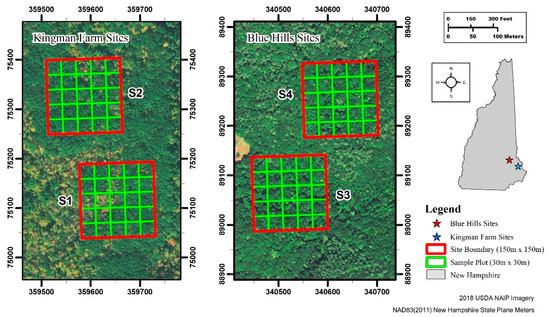
Figure 1.
Map of study sites and relative location within New Hampshire. The label next to each site is a unique identifier for that site. Site boundaries are 150 m × 150 m. Two sites were established in the University of New Hampshire Kingman Farm Research Forest in Madbury, NH, USA (see Sites S1 and S2) and other two in the Blue Hills Foundation conservation lands in Strafford, NH, USA (see Sites S3 and S4). Sample plots within each site are 30 m × 30 m. Ground data were collected at the center of each sample plot.
Each site was further divided into twenty-five, 30 m × 30 m (0.09 ha) square plots, 100 in total, for ground data collection. These forest stands are considered natural, midsuccessional, transition, and central hardwood—hemlock—and white pine forest communities [55]. Eastern hemlock (Tsuga canadensis (L.) Carr.) and white pine (Pinus strobus L.) are the usual dominant tree species in these communities. However, they made up a very small proportion of the composition within the study sites. The study sites were predominately composed of red maple (Acer rubrum L.), red oak (Quercus rubra L.), and American beech (Fagus grandifolia Ehrh.) with black birch (Betula lent, L.), yellow birch (Betula alleghaniensis Britt.) and paper birch (Betula papyrifera Marsh.) present in smaller quantities. There was a lack of midcanopy trees expected in a small area of Blue Hills where there was evidence of past harvesting. Ocular estimates of canopy cover across all sites were 80% or more.
2.2. Ground Data Collection
Trees were sampled at each 30 m × 30 m plot within the four study sites on the ground using horizontal point sampling [56] between January and July 2021. The center of the sample plots was located and marked on the ground using an EOS Arrow 100 GPS unit (Eos Positioning Systems Inc, Terrebonne, QC, Canada). The EOS Arrow 100 collects submeter accuracy data when connected to a satellite-based augmentation system (SBAS) (https://eos-gnss.com/products/hardware/arrow-100; last accessed 25 July 2021). To maximize the positional accuracy, plot centers were located during leaf-off to improve the receiver’s visibility to the sky and reduce multipath errors. Trees were determined “in” the plot using a basal area factor (BAF) of 40 for the Kingman Farm sites and 20 for the Blue Hills sites. A different BAF was required for each location due to differing stem density and diameter distributions and to achieve the goal of sampling approximate 3–4 trees per plot on average. Because UAS-SfM-generated point clouds do not sample vegetation below dense canopies, suppressed trees, trees whose canopy receives no direct sunlight [57], were not included. The height to the top of the crown of the included trees were measured with a Haglöf Vertex IV hypsometer (Haglöf Sweden AB, Långsele, Sweden). Three height measurements were taken for each tree and the average recorded as the final height. The average height of all the trees within each plot was then taken as the top-of-canopy height (TCH) for that plot.
2.3. UAS Data Collection
All flights were carried out with a senseFly eBee X fixed-wing UAS and a senseFly Aeria X camera (AgEagle Aerial Systems Inc, Wichita, KS, USA). The Aeria X uses a 24-megapixel APS-C sensor, an 18.5 mm (35 mm equivalent focal length of 28 mm) focal length lens, and a global shutter. All mission planning was controlled using senseFly eMotion 3 software [58]. A polygon of each study site was uploaded into the software program. The user set the desired flying heights and overlaps (side and forward overlap). The software tool then automatically determined the flight line locations, flight speed (cruising speeds between 11 and 30 m/s), and camera trigger time that meets the desired parameters.
In this study, three flying heights and four levels of forward overlap were tested (Table 1). Side overlap was not tested in this study as it has been found to not have a significant impact on height accuracy in similar studies [33]. Additionally, increasing the side overlap adds considerable time to the mission and data processing (more flight lines and images). For these reasons, a singular side overlap of 80% was set for all missions. This value has been found through personal testing to provide reliable reconstructions under varying conditions. For each site, the UAS collected imagery using all combinations of flying height and overlap resulting in 12 missions (i.e., independent image collections at a set flying height and overlap) for each site. In total 48 missions, were carried out (3 flying heights × 4 levels of overlap × 4 study sites).

Table 1.
Flying parameters tested in this study. The value in parenthesis is the nominal spatial resolution for that height given by senseFly eMotion Software.
Table 2 shows the collection dates for each site (S1–S4). Data collection was conducted during the peak of the growing season and within a single day for each plot to ensure environmental conditions were consistent within the site. While weather was not a directly controlled factor in this study, it is important to note that data collection was held on either completely overcast or clear days with calm wind speeds. For collections on clear days, every effort was made to fly as close to solar noon as possible to reduce shadowing. Flight records recorded during the missions show wind speeds, as measured by the UAS while flying, were typically less than 5 m/s with a peak of 6 m/s on one day.
Table 2.
Collection dates for the study sites.
2.4. UAS Image Processing
The eBee X is real-time kinematic/postprocessed kinematic (RTK/PPK)-enabled. Therefore, the raw GPS positions for each image can be postprocessed to improve the positional accuracy. The senseFly Flight Data Manager within eMotion software was used to conduct the PPK postprocessing with RINEX data provided by a nearby continuously operating reference station (CORS). Due to the high canopy cover in the study area, it was not possible to set ground control points (GCPs) as they would not be visible in the imagery. Final positional accuracies reported by eMotion software following the PPK postprocessing were approximately 3 cm and 7 cm for the imagery collected within the Kingman Farm and Blue Hills areas, respectively. The difference in final positional accuracy was an effect of the distance between the study sites and the chosen CORS station. The positional accuracy of the Kingman Farm sites was higher because they were closer to the CORS station.
The imagery was then processed using Agisoft Metashape Professional [59]. Agisoft Metashape is a leading software package for implementing the SfM process. The process begins by first identifying unique features (key points) within the individual images based on image texture. The software then matches key points across the overlapping images. The matched key points, now known as tie points, are then used to estimate the camera’s internal and external orientation parameters; necessary for estimating the coordinates and heights of the tie points. This results in what is known as the sparse point cloud and only includes the positions for the tie points. A second process known as multiview stereo (MVS) is then run to densify the sparse point cloud and enhance the amount of information extracted. The result of this process is known as the dense point cloud.
Each independent combination of flying heights within each site (48 missions) was processed using the same parameters for consistency. The specific Agisoft workflow and parameters are described here and shown in Table 3. Align photos was run on “High Accuracy” with Generic preselection, Reference preselection, and Adaptive model fitting turned on. No key-point or tie-point limit was set due to the difficultly in generating and matching unique features in areas that are highly homogenous in texture (i.e., all trees). While decreasing this limit can increase the computation time, it allows the software package to generate more key points and can improve the probability of identifying tie points. The dense point cloud creation was also run on “High Accuracy” with moderate point filtering.
Table 3.
Pertinent Agisoft Metashape Pro parameters. Unless specified below, all other values were kept at software default.
Each dense point cloud was normalized using a LiDAR-produced digital terrain model (DTM). Photogrammetrically produced point clouds have a difficult time capturing the terrain in areas with a dense canopy cover, such as the sites in this study, which can lead to inaccurate DTMs for normalization [33,60,61]. Consequently, externally produced DTMs are commonly used to normalize the point clouds to height above the ground [33,50,62]. LiDAR-produced DTMs (1 m and 2 m spatial resolution for Blue Hills and Kingman Farm, respectively) covering the study sites were downloaded from the GRANIT LiDAR Distribution Site (site https://lidar.unh.edu/map/, last accessed 7 September 2022). The elevation of the ground at the pixel within which each point fell was subtracted from the elevation of the point. To ensure a comparable vertical reference was used for all four sites, the vertical data of the DTMs were converted to NAVD88 (Geoid 12b) (current at the time of data creation) to match the UAS point clouds using the NOAA VDatum tool (https://vdatum.noaa.gov/, last accessed 7 September 2022).
2.5. UAS-Based Plot Height Estimates
For each plot at each site (100 total plots), an estimate of TCH was assessed for each flight combination to compare to the ground-based estimates. The LidR package [63] in R 4.0.2 [64] was used to process the point cloud datasets. All of the normalized point clouds for each site were clipped to the boundaries of each plot resulting in a point cloud for all flight combinations at the plot level (100 plots × 3 flying heights × 4 levels of overlap). For each plot and each flight combination (flying height and overlap), the common height-based point cloud metrics were extracted using the cloud_metrics function. The point cloud metrics included average height, maximum height, and height percentiles (i.e., the height below which p% of the points fall) between 5% and 95% using a 5% interval. The most correlated metric with the ground estimates of TCH was chosen to represent the plot-level estimate of TCH from the point clouds. Unlike LiDAR, the SfM process can result in voids in the point cloud where features could not be reconstructed. For each flying height, the point cloud associated with the most complete DSM was chosen to run the correlations against the ground data [53]. For all flight combinations, the respective DSM was exported and clipped to the site boundary. The completeness of each DSM was represented as the proportion of the pixels containing data values (i.e., was not null). As demonstrated in Frey et al. [53], this method is superior to point density as a measure of reconstruction success, as it takes into account that multiple points can exist within one pixel. Therefore, completeness gives an indication of the spread of those points across the area of interest. For each flying height, the correlation between height metrics for the point cloud with the greatest completeness and the ground was measured using Pearson’s correlation coefficient (r). The most correlated metric was chosen as the TCH estimate for each plot within the respective flying heights.
The accuracy of the point clouds from each flight combination was assessed by calculating the root-mean-square error of the TCH estimates (RMSETCH) using the ground and UAS TCH for the plots within each site. To clarify, within a single site, the RMSETCH was calculated at the plot level for all flight combinations. This analysis was repeated within each site resulting in twelve measures of RMSETCH (3 flying heights × 4 levels of overlap) with four replicates (n = 48).
2.6. Statistical Analysis
The effect of flying height and overlap on the accuracy of the TCH estimates was assessed by fitting a generalized linear model (GLM). The analysis was carried out in R 4.0.2 using the lme4 package [65]. RMSETCH was set as the response variable and the flying height and overlap as the predictors. Because of the use of site replicates and the fact that there was distinct difference in the terrain across sites, an ID (identification number) for each site was also included as a predictor to account for the site effects. Because RMSETCH values are bounded at the left side (RMSE cannot be lower than 0), a gamma distribution with a log link function was specified for the response. Two versions of the model were generated; the first included flying height and overlap as additive effects. The second incorporated an additional interaction term between flying height and overlap to account for the relationship between the ground area covered by the overlap and flying height. An Akaike information criterion (AIC) model comparison indicated that the model without the interaction term was more parsimonious. Additionally, the interaction was not found to be significant when it was included. Based on these results, the simpler model without the interaction term was chosen as the primary model for assessing the effects.
We note here that given this experimental design; an attempt was made to fit the data using a generalized linear mixed-effect model with the site set as a random effect. The model was unable to converge when a gamma distribution was specified. Thus, the decision was made to use the GLM with the site included as a fixed effect so it was accounted for and the normality assumption for the response could be maintained.
3. Results
3.1. Ground Data Summary
Table 4 presents a summary of the ground data collection at each site. In total, 425 trees were measured across the four sites. It is important to note that the number of trees measured in each plot varied based on the stem density and the diameter at breast height (DBH) at the plot. Different BAFs were used to keep the sampling intensity roughly equal across the plots and the sites, which was successful based on the similarity in the average trees measured across the plots.
Table 4.
Summary of ground data collection for all four sites. Standard deviation is given in parentheses for all means.
3.2. Point Cloud Completeness and Correlations
The completeness of the DSMs was calculated for all flight combinations. The results are presented in Figure 2. Completeness exhibited an increase with increasing flying height, thus was the lowest at 80 m and the highest at 120 m above the canopy. Completeness exhibited a distinct peak at 85% overlap before dropping again. Only the 100 m and 120 m flying heights began to exhibit an increase again after 90% overlap.
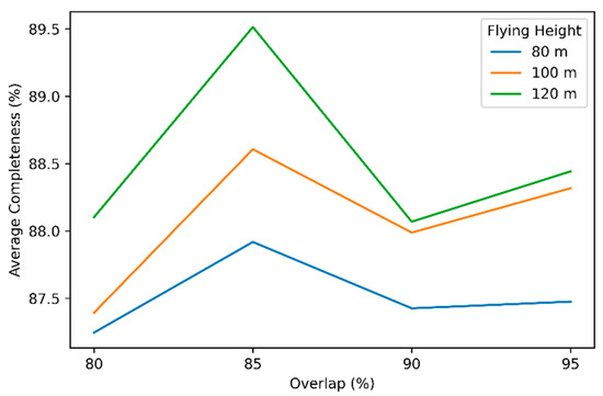
Figure 2.
Change in the average completeness with forward overlap and flying height.
The 85% forward overlap for each flying height was used to run the correlation between the point cloud metrics and the ground data. For each flying height, the highest correlation was found with the 85th height percentile. The Pearson’s correlation parameter was 0.838, 0.839, and 0.839 for 120 m, 100 m, and 80 m, respectively. All correlations were significant at the 95% confidence interval. Thus, the 85th percentile height was taken as the height estimate at each site for all flight configurations.
3.3. Effect of Flight Parameters on TCH Accuracy
The RMSETCH across all sites and flight parameter combinations ranged between 1.75 m (RMSETCH % = 5.94%) and 3.20 m (RMSETCH % = 12.4%). A comparison of the per-plot estimates to the ground reference showed consistent underestimation of the ground estimated tree height (mean error of −1.03 m). The change in RMSETCH, in both meters and percent, with flying height and overlap are summarized in Table 5 and Table 6, respectively, and the coefficients and p-values of the selected GLM model are shown in Table 7. The values in Table 5 and Table 6 represent the average and standard deviation for the four sites. There was no consistent pattern in RMSETCH with flying height. Forward overlap exhibited a slight decrease in RMSETCH with increasing overlap. The GLM model found no significant difference in RMSETCH with flying height and a significant decrease in RMSETCH with increasing forward overlap. Based on the model coefficients, a 4 mm decrease in RMSETCH was expected with a 1% increase in overlap.
Table 5.
RMSETCH across the levels of flying height and forward overlap in meters. Values are the mean and standard deviation (in parentheses) for the four sites. Marginal values are row and column averages.
Table 6.
RMSETCH across the levels of flying height and forward overlap in relative (%) values. Values are the mean and standard deviation (in parentheses) for the four sites. Marginal values are row and column averages.
Table 7.
Output of the chosen GLM model. Coefficients are on the response scale. Significance of the predictor is indicated with asterisks (*).
4. Discussion
4.1. Point Cloud Completeness
The relationship between DSM completeness, flying height, and forward overlap exhibited two notable trends. First, there was an increase in DSM completeness with increased flying height and second, there was a distinct peak at 85% overlap for all three flying heights. The increase in completeness with flying height was in line with the results of several studies that have investigated levels of scene reconstruction with changing flight parameters [50,51,53,66]. These studies found that reconstruction was improved by flying higher, due to the decrease in image texture that occurs as the spatial resolution decreases [5,46,50]. Westoby et al. [32] noted that the reconstruction of a scene was difficult when there was a high level of homogeneity in texture across the overlapping images. This may include either highly repetitive or monochromatic texture [67]. Decreasing the texture makes it easier for the computer vision algorithms to locate unique features that can be accurately matched. In terms of the peak at 85%, increasing forward overlap has been found to increase point density [33,51]. Increasing the overlap increases the chances of finding image matches and adjusts the viewing angle, which can change texture [50,53]. Frey et al. [53], however, found a continuously increasing completeness with increasing overlap. They adjusted their forward overlap by systematically removing photos along each flight line and their spatial resolution by upscaling the original imagery to coarser spatial resolutions, breaking the relationship between flying height and area covered by the image overlap. In this study, each level of overlap and flying height was independently collected.
The base-to-height (B/H) ratio is the relationship between flying height and the distance between the centers of two overlapping photos. B/H has long been an important parameter in traditional photogrammetry due to its impact on the estimate of height [68]. Goldbergs [69] demonstrated the importance of the B/H ratio for estimating the height and completeness, noted here as the ability to detect reference trees, using photogrammetrically derived DSMs from airborne and satellite imagery. An important conclusion of that study was that the B/H ratio had significant control on the completeness of the DSM and suggested B/H values between 0.2 and 0.3 for accurate reconstruction of the canopy in closed-canopy forests. These values approximately equate with forward overlaps between 64% and 75% with the Aeria X camera used in this study. While these values were not tested here, it is important to note that at an 85% forward overlap, every other photo on a flight line overlaps by 70%, which corresponds to a B/H of 0.247. Furthermore, the B/H of the side lap utilized across all flight configurations, 80%, was also 0.247, potentially compounding the improvement. Table 5 suggests that B/H might still be important in terms of accuracy as well for UAS-SfM. RMSETCH dropped when the forward overlap increased to 85% and increased at 90% forward overlap. Goldbergs [69] found tree height accuracy was improved at optimal B/H ratios. A thorough analysis of this result is beyond the scope of the study but suggests that more work is needed to understand the relationship between B/H and the photogrammetric output with UAS as it could go a long way towards making suitable flight parameter choices.
4.2. Tree Height Accuracy
The RMSETCH ranged between 1.75 m (RMSETCH % = 5.94%) and 3.20 m (RMSETCH % = 12.4%) across all sites and tested flight parameters. These values are consistent with previous studies. Lisein et al. [34] and Dandois et al. [46] reported an RMSE of 1.65 (RMSE% = 8.4%) and 3.3 m (no relative RMSE reported), respectively, for the predominate height estimated using a fixed-wing UAS over natural deciduous-dominated stands with minimal variation in terrain, similar to the current study area. Their errors were higher potentially because they utilized the average of the canopy height model as their UAS metric for TCH, yet their ground estimates were based on the predominate trees in their plots. Nasiri et al. [70] measured an RMSE of 3.22 m (RMSE% = 10.1%) in a deciduous-dominated, complex, mountainous forest in northern Iran. Jayathunga et al. [36] reported an RMSE of 1.78 m in a complex, mixed conifer–broadleaf forest. We are taking care to note the forest type of the mentioned studies because forest type could very well have an impact on accuracy. Puliti et al. [35] and Li et al. [71] reported RMSEs of 0.71 m (RMSE% = 3.6%) and 1.01 m (RMSE% = 6.60%) in boreal forest stands and conifer plantations, respectively, with simpler structures relative to this study. He et al. [38] achieved an RMSE of 9.24 cm in a mountainous forest plantation in China.
The underestimation found in this study (mean error of -1.03 m) is an often-reported result when using UAS-SfM to estimate tree height [33,34,72,73]. On the ground, tree height is typically taken as the topmost point on the canopy. It may be possible to see fine peaks, possibly branches, at the top of the canopy that could very well not be detected during the SfM process [36]. It should also be noted here that the ground data for Kingman Farm was collected during leaf-off conditions which could have led to lower ground measured tree heights compared to data collected during leaf-on periods. Assuming the UAS-SfM heights were already underestimated, the error at those sites would be less. Indeed, the average error for the sites collected in winter was less than that of the summer, −0.67 m versus −1.16 m, respectively. Furthermore, there can be substantial error when making the field measurements due to the difficultly of locating the top of the trees. Ganz et al. [73] found height measurements taken indirectly with a Vertex hypsometer had a mean error of −0.66 m and RMSE of 1.02 m when compared to direct measurements after felling the measured trees. Additionally, they found the variation in the hypsometer measurements to be much higher when compared to the estimates made from remotely sensed data, including UAS-SfM products.
4.3. Flight Parameter Effects on Tree Height RMSE
The interpretation of the values in Table 5 was confirmed by the results of the GLM model (Table 7). Flying height had no significant effect on RMSETCH but was found to significantly decrease with increasing forward overlap. While significant, however, the effect was minor, only a 4 mm decrease per 1% forward overlap increase. Dandois et al. [33] also implemented a fully factorial study of flight parameters on TCH over deciduous forest stands and found flying height had no significant effect, while increasing forward overlap led to a significant decrease in RMSE. Kameyama and Sugiura [37] similarly found little change in the accuracy of individual tree height estimates with differing flying heights. Torres-Sánchez et al. [49] also found increasing forward overlap increased the accuracy of individual tree height estimates. It is worth noting that Torres-Sánchez et al. [69] also showed very little change in the error between forward overlaps of 80% and 95%.
Table 7 did not include the GLM results for the site variable, but a discussion of site is still relevant. A significant difference in RMSETCH was found for all four sites. There are a number of reasons for this. First, the individual physical differences in the sites themselves have an impact on the structure of the forest, which was not investigated here. Second, these differences could also affect the ability to make accurate measurements on the ground. The Kingman Farm sites for example were on much flatter terrain relative to the Blue Hills sites, which were much steeper. Additionally, while an attempt was made to perform the UAS data collection under similar conditions, there were still variations in the imagery due to differences in lighting and/or wind. While these factors could impact accuracy, the utilization of site replicates lends a greater credibility to the results.
The considerable effect of increased overlap is often attributed to a better reconstruction of the scene due to the increased probability of locating matching features [33,51,53,72]. In general, by increasing overlap, the search area for matching features is increased. Frey et al. [53] found that the completeness of the model increased with increasing forward overlap for all spatial resolutions that were tested. Kameyama and Sugiura [37] also noted that 3D reconstruction was more complete as overlap increased. Our study examined a narrow range of possible overlaps, less so than other studies [33,50,53]. While a significant effect was detected, the effect was minimal. Larger differences may be measured if overlaps less than 80% are tested; however, it has been found that the estimation of the camera parameters begins to fail as forward overlap decreases, resulting in highly incomplete models [66].
The nonsignificance of flying height on the accuracy of tree height measurements could be the result of the narrow difference in spatial resolution within the flying heights tested. Based on the nominal spatial resolution provided by senseFly eMotion software, there is only a 0.85 cm difference between the 80 m and 120 m flying height. The spatial resolution range for Dandois et al. [33] was only 2.6 cm. Frey et al. [53] also showed that the spatial resolution of the imagery had a minimal impact on the completeness of the models at higher (>80%) levels of forward overlap. Furthermore, TCH may not be very sensitive to flying height. Ni et al. [50] assessed changes in the vertical distribution of the SfM point cloud across a wider range of spatial resolutions (8.6 cm to 1.376 m) via image upscaling and found that for high-density forests, as the spatial resolution increased, the vertical distribution narrowed but remained centered on the upper canopy. This result suggests the top of the canopy is accurately reconstructed across a number of flying heights. Structural metrics that rely on estimates from lower in the canopy, especially the ground, may find a greater effect with flying height as it has been found that lower flying heights are needed to accurately reconstruct the lower levels of the canopy [33,50,53].
4.4. Limitations
This study only investigated the effects of forward overlap and flying height on the accuracy of canopy height. Additionally, the composition of the forest across the plots were similar. Other factors such as light condition, wind speed, camera type, slope, etc., with known impacts on the 3D reconstruction were not investigated [31,33]. It is also important to note the UAS utilized in this study. It has been suggested that UASs with gimbals are useful because they stabilize the camera during the mission, better ensuring the imagery is nadir [31]. The eBee X lacks a gimbal and thus the imagery was often off-nadir (i.e., nonvertical or oblique) due to crosswinds. The user-defined overlap is only achieved when images are vertical, thus oblique images change the realized overlap across the mission area. However, these images may present an advantage when estimating tree height as it has been suggested that the inclusion of oblique imagery can improve the accuracy of forest structural estimates by providing more angles of the individual trees [40].
The distance between successive photos on a flight line decrease with decreasing flying height and increasing forward overlap. Consequently, a UAS must slow down to ensure the previous image is captured and stored before reaching the location of the next. A fixed wing UAS must maintain a certain speed, however, to guarantee proper flight capabilities. Therefore, if the UAS cannot slow down enough, photos are either skipped or taken later than planned. The inability to achieve certain levels of overlap may explain why the completeness of the DSMs at an 80 m flying height did not improve again after 90% forward overlap as for the 100 m and 120 m flying heights. The distance between two photos is only 3.3 m at a flying height and forward overlap of 80 m and 95%, respectively. With a minimum cruise speed of 11 m/s, it would take the eBee X used in this study 0.3 s to reach the next photo under perfect conditions.
4.5. Implications
Based on the results of this study, two suggestions can be made about the choice of flight parameters. We note here that these results should be considered within the context of this study (i.e., UAS type, parameters tested, forest type). Flying with higher levels of forward overlap will increase the accuracy of the height estimates from the SfM point cloud; however, the increase is potentially minimal. While completeness was not a focus of this study, the results of both the RMSETCH and the completeness investigations suggest that perhaps the highest overlap is not necessary. This is especially helpful at lower flying altitudes where the distance between photos is shorter. Additionally, flying height can be set higher without any significant impact on accuracy of dominant height measurements. Unlike a rotary wing UAS, flying heights for a fixed-wing UAS are more restrictive due to the nature of how it flies. For example, a fixed-wing UAS performs banking turns, placing it closer to the canopy. Additionally, a fixed-wing UAS cannot stop midflight in the event of an obstruction, so the user must set a safe flying height. The ability to fly higher without sacrificing accuracy is a benefit both in terms of time and safety. The combination of a lower overlap and flying higher would save time both flying and processing the data, by decreasing the number of images that need to be collected.
5. Conclusions
UAS have the potential to be an important tool in our efforts to conduct more sustainable forest management by providing three-dimensional information about a forest in a timelier manner and with significantly reduced costs relative to traditional remote sensing platforms. A useful approach to extracting this information is through the SfM process. The ability to create 3D data with simple aerial imagery rather than expensive LiDAR sensors is a significant advantage. However, because the SfM process relies on the ability to detect matching features within the overlapping sections of the imagery, it is sensitive to the quality and geometry of the imagery and its collection, a sensitivity which must be understood. The objective of this study was to investigate the effects of flying height and overlap on plot level estimates of top-of-canopy height (TCH). Three flying heights and four levels of forward overlap were flown across four predominately deciduous forest plots. Estimates of TCH for each combination of flight parameters were compared to ground estimates. It was then determined if either parameter had a significant effect on the RMSE of the TCH (RMSETCH) estimates.
Across all flight configurations and sites, the RMSETCH ranged between 1.75 m and 3.20 m. Tree height was typically underestimated by the UAS. Underestimation could be an effect of measurement error on the ground or the inability of the SfM process to properly detect and reconstruct the very tops of trees. There was no significant effect of flying height on accuracy which could be due to the minimal variation in the spatial resolutions across the studied flying heights. Additionally, it is possible that reconstruction of the tops of trees is robust to the spatial resolution used. A significant, but minor, effect of forward overlap was detected. Increasing the forward overlap has been shown to improve reconstruction by providing more overlap between images for feature matching.
Based on the results, a higher forward overlap would increase the accuracy of the results. The improvement would be minor, however, and this study provided some indication that the highest level of overlap may not be necessary. Furthermore, for estimating TCH, flying higher could save substantial time on data collection and image processing, with no real impact on TCH accuracy.
Author Contributions
H.G. conceived and designed the study, conducted the data collection and analysis, and wrote the first draft of the paper. R.G.C. contributed to the development of the overall research design, suggested improvements, and aided in the writing of the paper. All authors have read and agreed to the published version of the manuscript.
Funding
Partial funding was provided by the New Hampshire Agricultural Experiment Station. This is Scientific Contribution Number 2940. This work was supported by the USDA National Institute of Food and Agriculture McIntire-Stennis Project 1002519.
Acknowledgments
The authors would like to thank Jianyu Gu, Benjamin Fraser, and Molly Yanchuck for all their assistance with the ground and UAS data collection and the Blue Hills Foundation Inc. for permission to conduct this study on their lands.
Conflicts of Interest
The authors declare no conflict of interest.
References
- The North East State Foresters Association (NEFA). The Economic Imortance of New Hampshire’s Forest-Based Economy. 2013. Available online: https://www.nefainfo.org/uploads/2/7/4/5/27453461/nefa13_econ_importance_nh_final_web.pdf (accessed on 25 July 2021).
- Food and Agricultural Organization of the United Nations. United Nations Environment Programme The State of the World’s Forests 2020. In Forests, Biodiversity and People; FAO; UNEP: Rome, Italy, 2020; ISBN 978-92-5-132419-6. [Google Scholar]
- Turunen, J.; Elbrecht, V.; Steinke, D.; Aroviita, J. Riparian Forests Can Mitigate Warming and Ecological Degradation of Agricultural Headwater Streams. Freshw Biol. 2021, 66, 785–798. [Google Scholar] [CrossRef]
- Goodale, C.L.; Apps, M.J.; Birdsey, R.A.; Field, C.B.; Heath, L.S.; Houghton, R.A.; Jenkins, J.C.; Kohlmaier, G.H.; Kurz, W.; Liu, S.; et al. Forest Carbon Sinks in the Northern Hemisphere. Ecol. Appl. 2002, 12, 891–899. [Google Scholar] [CrossRef]
- MacDicken, K.G.; Sola, P.; Hall, J.E.; Sabogal, C.; Tadoum, M.; de Wasseige, C. Global Progress toward Sustainable Forest Management. For. Ecol. Manag. 2015, 352, 47–56. [Google Scholar] [CrossRef]
- White, J.C.; Coops, N.C.; Welder, M.A.; Vastaranta, M.; Hilker, T.; Tompalski, P. Remote Sensing Technologies for Enhancing Forest Inventories: A Review. Can. J. Remote Sens. 2016, 42, 619–641. [Google Scholar] [CrossRef]
- Hilker, T.; Wulder, M.A.; Coops, N.C. Update of Forest Inventory Data with Lidar and High Spatial Resolution Satellite Imagery. Can. J. Remote Sens. 2008, 34, 5–12. [Google Scholar] [CrossRef]
- Brosofske, K.D.; Froese, R.E.; Falkowski, M.J.; Banskota, A. A Review of Methods for Mapping and Prediction of Inventory Attributes for Operational Forest Management. For. Sci. 2014, 60, 733–756. [Google Scholar] [CrossRef]
- Goodbody, T.R.H.; Coops, N.C.; White, J.C. Digital Aerial Photogrammetry for Updating Area-Based Forest Inventories: A Review of Opportunities, Challenges, and Future Directions. Curr. For. Rep. 2019, 55–75. [Google Scholar] [CrossRef]
- Iglhaut, J.; Cabo, C.; Puliti, S.; Piermattei, L.; O’Connor, J.; Rosette, J. Structure from Motion Photogrammetry in Forestry: A Review. Curr. For. Rep. 2019, 5, 155–168. [Google Scholar] [CrossRef]
- Dainelli, R.; Toscano, P.; di Gennaro, S.F.; Matese, A. Recent Advances in Unmanned Aerial Vehicles Forest Remote Sensing—A Systematic Review. Part i: Research Applications. Forests 2021, 12, 397. [Google Scholar] [CrossRef]
- Loarie, S.R.; Joppa, L.N.; Pimm, S.L. Satellites Miss Environmental Priorities. Trends Ecol. Evol. 2007, 22, 630–632. [Google Scholar] [CrossRef]
- Wiens, J.; Sutter, R.; Anderson, M.; Blanchard, J.; Barnett, A.; Aguilar-Amuchastegui, N.; Avery, C.; Laine, S. Selecting and Conserving Lands for Biodiversity: The Role of Remote Sensing. Remote Sens. Environ. 2009, 113, 1370–1381. [Google Scholar] [CrossRef]
- Anderson, K.; Gaston, K.J. Lightweight Unmanned Aerial Vehicles Will Revolutionize Spatial Ecology. Front. Ecol. Environ. 2013, 11, 138–146. [Google Scholar] [CrossRef]
- Wulder, M.A.; White, J.C.; Nelson, R.F.; Næsset, E.; Ørka, H.O.; Coops, N.C.; Hilker, T.; Bater, C.W.; Gobakken, T. Lidar Sampling for Large-Area Forest Characterization: A Review. Remote Sens. Environ. 2012, 121, 196–209. [Google Scholar] [CrossRef]
- Guimarães, N.; Pádua, L.; Marques, P.; Silva, N.; Peres, E.; Sousa, J.J. Forestry Remote Sensing from Unmanned Aerial Vehicles: A Review Focusing on the Data, Processing and Potentialities. Remote Sens. 2020, 12, 1046. [Google Scholar] [CrossRef]
- Lim, K.; Treitz, P.M.; Wulder, M.A.; St-Onge, B.; Flood, M. LiDAR Remote Sensing of Forest Structure. Prog. Phys. Geogr. 2003, 27, 88–106. [Google Scholar] [CrossRef]
- Lefsky, M.A.; Cohen, W.B.; Acker, S.A.; Parker, G.G.; Spies, T.A.; Harding, D. Lidar Remote Sensing of the Canopy Structure and Biophysical Properties of Douglas-Fir Western Hemlock Forests. Remote Sens. Environ. 1999, 70, 339–361. [Google Scholar] [CrossRef]
- Næsset, E. Predicting Forest Stand Characteristics with Airborne Scanning Laser Using a Practical Two-Stage Procedure and Field Data. Remote Sens. Environ. 2002, 80, 88–99. [Google Scholar] [CrossRef]
- Vega, C.; Hamrouni, A.; el Mokhtari, A.; Morel, M.; Bock, J.; Renaud, J.P.; Bouvier, M.; Durrieue, S. PTrees: A Point-Based Approach to Forest Tree Extractionfrom Lidar Data. Int. J. Appl. Earth Obs. Geoinf. 2014, 33, 98–108. [Google Scholar] [CrossRef]
- Arumäe, T.; Lang, M. Estimation of Canopy Cover in Dense Mixed-Species Forests Using Airborne Lidar Data. Eur. J. Remote Sens. 2018, 51, 132–141. [Google Scholar] [CrossRef]
- White, J.C.; Wulder, M.A.; Varhola, A.; Vastaranta, M.; Coops, N.C.; Cook, B.D.; Pitt, D.; Woods, M. A best practices guide for generating forest inventory attributes from airborne laser scanning data using an area-based approach. For. Chron. 2013, 89, 722–723. [Google Scholar] [CrossRef] [Green Version]
- Ota, T.; Ogawa, M.; Shimizu, K.; Kajisa, T.; Mizoue, N.; Yoshida, S.; Takao, G.; Hirata, Y.; Furuya, N.; Sano, T.; et al. Aboveground Biomass Estimation Using Structure from Motion Approach with Aerial Photographs in a Seasonal Tropical Forest. Forests 2015, 6, 3882–3898. [Google Scholar] [CrossRef]
- Latifi, H.; Nothdurft, A.; Koch, B. Non-Parametric Prediction and Mapping of Standing Timber Volume and Biomass in a Temperate Forest: Application of Multiple Optical/LiDAR-Derived Predictors. Forestry 2010, 83, 395–407. [Google Scholar] [CrossRef]
- Næsset, E.; Bollandsas, O.M.; Gobakken, T. Comparing Regression Methods in Estimation of Biophysical Properties of Forest Stands from Two Different Inventories Using Laser Scanner Data. Remote Sens. Environ. 2005, 94, 541–553. [Google Scholar] [CrossRef]
- Jayathunga, S.; Owari, T.; Tsuyuki, S.; Hirata, Y. Potential of UAV Photogrammetry for Characterization of Forest Canopy Structure in Uneven-Aged Mixed Conifer–Broadleaf Forests. Int. J. Remote Sens. 2020, 41, 53–73. [Google Scholar] [CrossRef]
- Wulder, M.A.; Coops, N.C.; Hudak, A.T.; Morsdorf, F.; Nelson, R.F.; Newnham, G.J.; Vastaranta, M. Status and Prospects for LiDAR Remote Sensing of Forested Ecosystems. Can. J. Remote Sens. 2013, 39, S1–S5. [Google Scholar] [CrossRef]
- Beland, M.; Parker, G.; Sparrow, B.; Harding, D.; Chasmer, L.; Phinn, S.; Antonarakis, A.; Strahler, A. On Promoting the Use of Lidar Systems in Forest Ecosystem Research. For. Ecol. Manag. 2019, 450, 117484. [Google Scholar] [CrossRef]
- Gould, W. Remote Sensing of Vegetation, Plant Species Richness, and Regional Biodiversity Hotspots. Ecol. Appl. 2000, 10, 1861–1870. [Google Scholar] [CrossRef]
- Wulder, M.A.; Hall, R.J.; Coops, N.C.; Franklin, S.E. High Spatial Resolution Remotely Sensed Data for Ecosystem Characterization. Bioscience 2004, 54, 511–521. [Google Scholar] [CrossRef]
- Cruzan, M.B.; Weinstein, B.G.; Grasty, M.R.; Kohrn, B.F.; Hendrickson, E.C.; Arredondo, T.M.; Thompson, P.G. Small Unmanned Aerial Vehicles (Micro-Uavs, Drones) in Plant Ecology. Appl. Plant Sci. 2016, 4, 1600041. [Google Scholar] [CrossRef]
- Westoby, M.J.; Brasington, J.; Glasser, N.F.; Hambrey, M.J.; Reynolds, J.M. “Structure-from-Motion” Photogrammetry: A Low-Cost, Effective Tool for Geoscience Applications. Geomorphology 2012, 179, 300–314. [Google Scholar] [CrossRef] [Green Version]
- Dandois, J.P.; Olano, M.; Ellis, E.C. Optimal Altitude, Overlap, and Weather Conditions for Computer Vision Uav Estimates of Forest Structure. Remote Sens. 2015, 7, 13895–13920. [Google Scholar] [CrossRef]
- Lisein, J.; Pierrot-Deseilligny, M.; Bonnet, S.; Lejeune, P. A Photogrammetric Workflow for the Creation of a Forest Canopy Height Model from Small Unmanned Aerial System Imagery. Forests 2013, 4, 922–944. [Google Scholar] [CrossRef]
- Puliti, S.; Olerka, H.; Gobakken, T.; Næsset, E.; Ørka, H.O.; Gobakken, T.; Næsset, E.; Olerka, H.; Gobakken, T.; Næsset, E. Inventory of Small Forest Areas Using an Unmanned Aerial System. Remote Sens. 2015, 7, 9632–9654. [Google Scholar] [CrossRef]
- Jayathunga, S.; Owari, T.; Tsuyuki, S. Evaluating the Performance of Photogrammetric Products Using Fixed-Wing UAV Imagery over a Mixed Conifer-Broadleaf Forest: Comparison with Airborne Laser Scanning. Remote Sens. 2018, 10, 187. [Google Scholar] [CrossRef]
- Kameyama, S.; Sugiura, K. Estimating Tree Height and Volume Using Unmanned Aerial Vehicle Photography and Sfm Technology, with Verification of Result Accuracy. Drones 2020, 4, 19. [Google Scholar] [CrossRef]
- He, H.; Yan, Y.; Chen, T.; Cheng, P. Tree Height Estimation of Forest Plantation in Mountainous Terrain from Bare-Earth Points Using a DoG-Coupled Radial Basis Function Neural Network. Remote Sens. 2019, 11, 1271. [Google Scholar] [CrossRef]
- Bonnet, S.; Lisein, J.; Lejeune, P. Comparison of UAS Photogrammetric Products for Tree Detection and Characterization of Coniferous Stands. Int. J. Remote Sens. 2017, 38, 5310–5337. [Google Scholar] [CrossRef]
- Swayze, N.C.; Tinkham, W.T.; Vogeler, J.C.; Hudak, A.T. Influence of Flight Parameters on UAS-Based Monitoring of Tree Height, Diameter, and Density. Remote Sens. Environ. 2021, 263, 112540. [Google Scholar] [CrossRef]
- Domingo, D.; Ørka, H.O.; Næsset, E.; Kachamba, D.; Gobakken, T. Effects of UAV Image Resolution, Camera Type, and Image Overlap on Accuracy of Biomass Predictions in a Tropicalwoodland. Remote Sens. 2019, 11, 948. [Google Scholar] [CrossRef]
- Nasiri, V.; Darvishsefat, A.A.; Arefi, H.; Griess, V.C.; Sadeghi, S.M.M.; Borz, S.A. Modeling Forest Canopy Cover: A Synergistic Use of Sentinel-2, Aerial Photogrammetry Data, and Machine Learning. Remote Sens. 2022, 14, 1453. [Google Scholar] [CrossRef]
- Safonova, A.; Hamad, Y.; Dmitriev, E.; Georgiev, G.; Trenkin, V.; Georgieva, M.; Dimitrov, S.; Iliev, M. Individual Tree Crown Delineation for the Species Classification and Assessment of Vital Status of Forest Stands from UAV Images. Drones 2021, 5, 77. [Google Scholar] [CrossRef]
- Panagiotidis, D.; Abdollahnejad, A.; Slavík, M. 3D Point Cloud Fusion from UAV and TLS to Assess Temperate Managed Forest Structures. Int. J. Appl. Earth Obs. Geoinf. 2022, 112, 102917. [Google Scholar] [CrossRef]
- Panagiotidis, D.; Abdollahnejad, A.; Surový, P.; Chiteculo, V. Determining Tree Height and Crown Diameter from High-Resolution UAV Imagery. Int. J. Remote Sens. 2017, 38, 2392–2410. [Google Scholar] [CrossRef]
- Dandois, J.P.; Ellis, E.C. High Spatial Resolution Three-Dimensional Mapping of Vegetation Spectral Dynamics Using Computer Vision. Remote Sens. Environ. 2013, 136, 259–276. [Google Scholar] [CrossRef]
- Manfreda, S.; McCabe, M.F.; Miller, P.E.; Lucas, R.; Madrigal, V.P.; Mallinis, G.; ben Dor, E.; Helman, D.; Estes, L.; Ciraolo, G.; et al. On the Use of Unmanned Aerial Systems for Environmental Monitoring. Remote Sens. 2018, 10, 641. [Google Scholar] [CrossRef]
- Whitehead, K.; Hugenholtz, C.H. Remote Sensing of the Environment with Small Unmanned Aircraft Systems ( UASs ), Part 1: A Review of Progress and Challenges. J. Unmanned Veh. Syst. 2014, 2, 69–85. [Google Scholar] [CrossRef]
- Torres-Sánchez, J.; López-Granados, F.; Borra-Serrano, I.; Peña, J.M. Assessing UAV-Collected Image Overlap Influence on Computation Time and Digital Surface Model Accuracy in Olive Orchards. Precis. Agric. 2017, 19, 115–133. [Google Scholar] [CrossRef]
- Ni, W.; Sun, G.; Pang, Y.; Zhang, Z.; Liu, J.; Yang, A.; Wang, Y.; Zhang, D. Mapping Three-Dimensional Structures of Forest Canopy Using UAV Stereo Imagery: Evaluating Impacts of Forward Overlaps and Image Resolutions with LiDAR Data as Reference. IEEE J. Sel. Top. Appl. Earth Obs. Remote Sens. 2018, 11, 3578–3589. [Google Scholar] [CrossRef]
- de Lima, R.S.; Lang, M.; Burnside, N.G.; Peciña, M.V.; Arumäe, T.; Laarmann, D.; Ward, R.D.; Vain, A.; Sepp, K. An Evaluation of the Effects of UAS Flight Parameters on Digital Aerial Photogrammetry Processing and Dense-Cloud Production Quality in a Scots Pine Forest. Remote Sens. 2021, 13, 1121. [Google Scholar] [CrossRef]
- Tang, L.; Shao, G. Drone Remote Sensing for Forestry Research and Practices. J. For. Res. (Harbin) 2015, 26, 791–797. [Google Scholar] [CrossRef]
- Frey, J.; Kovach, K.; Stemmler, S.; Koch, B. UAV Photogrammetry of Forests as a Vulnerable Process. A Sensitivity Analysis for a Structure from Motion RGB-Image Pipeline. Remote Sens. 2018, 10, 912. [Google Scholar] [CrossRef]
- Goodbody, T.R.H.; Coops, N.C.; Marshall, P.L.; Tompalski, P.; Crawford, P. Unmanned Aerial Systems for Precision Forest Inventory Purposes: A Review and Case Study. For. Chron. 2017, 93, 71–81. [Google Scholar] [CrossRef]
- Westveld, M. Natural Forest Vegetation Zones of New England. J. For. 1956, 54, 332–338. [Google Scholar]
- Kershaw, J.A.; Ducey, M.J.; Beers, T.W.; Husch, B. Forest Mensuration, 5th ed.; John Wiley and Sons: Chichester, UK, 2016. [Google Scholar]
- Oliver, C.D.; Larson, B.C. Forest Stand Dynamics: Updated Edition; John Wiley and Sons: New York, NY, USA, 1996; ISBN 0471138339. [Google Scholar]
- SenseFly. EMotion User Manual Revision 3.1; v3.1; SensFly SA: Cheseaux-sur-Lausanne, Switzerland, 2020. [Google Scholar]
- Agisoft. Agisoft Metashape User Manual Professional Edition; Verision 1.6; Agisoft LLC: St. Petersburg, Russia, 2020. [Google Scholar]
- Wallace, L.; Bellman, C.; Hally, B.; Hernandez, J.; Jones, S.; Hillman, S. Assessing the Ability of Image Based Point Clouds Captured from a UAV to Measure the Terrain in the Presence of Canopy Cover. Forests 2019, 10, 284. [Google Scholar] [CrossRef]
- Graham, A.; Coops, N.C.; Wilcox, M.; Plowright, A. Evaluation of Ground Surface Models Derived from Unmanned Aerial Systems with Digital Aerial Photogrammetry in a Disturbed Conifer Forest. Remote Sens. 2019, 11, 84. [Google Scholar] [CrossRef]
- Hugenholtz, C.H.; Whitehead, K.; Brown, O.W.; Barchyn, T.E.; Moorman, B.J.; LeClair, A.; Riddell, K.; Hamilton, T. Geomorphological Mapping with a Small Unmanned Aircraft System (SUAS): Feature Detection and Accuracy Assessment of a Photogrammetrically-Derived Digital Terrain Model. Geomorphology 2013, 194, 16–24. [Google Scholar] [CrossRef]
- Roussel, J.R.; Auty, D.; Coops, N.C.; Tompalski, P.; Goodbody, T.R.H.; Meador, A.S.; Bourdon, J.F.; de Boissieu, F.; Achim, A. LidR: An R Package for Analysis of Airborne Laser Scanning (ALS) Data. Remote Sens. Environ. 2020, 251, 112061. [Google Scholar] [CrossRef]
- R Core Team. R: A Language and Environment for Statistical Computing; R Foundation for Statistical Computing: Vienna, Austria, 2020. [Google Scholar]
- Bates, D.; Mächler, M.; Bolker, B.M.; Walker, S.C. Fitting Linear Mixed-Effects Models Using Lme4. J. Stat. Softw. 2015, 67. [Google Scholar] [CrossRef]
- Fraser, B.T.; Congalton, R.G. Issues in Unmanned Aerial Systems (UAS) Data Collection of Complex Forest Environments. Remote Sens. 2018, 10, 908. [Google Scholar] [CrossRef]
- Bianco, S.; Ciocca, G.; Marelli, D. Evaluating the Performance of Structure from Motion Pipelines. J. Imaging 2018, 4, 98. [Google Scholar] [CrossRef]
- McGlone, J.C. Manual of Photogrammetry, 6th ed.; McGlone, J.C., Lee, G.Y.G., Eds.; American Society for Photogrammetry and Remote Sensing: Bethesda, MD, USA, 2013. [Google Scholar]
- Goldbergs, G. Impact of Base-to-Height Ratio on Canopy Height Estimation Accuracy of Hemiboreal Forest Tree Species by Using Satellite and Airborne Stereo Imagery. Remote Sens. 2021, 13, 2941. [Google Scholar] [CrossRef]
- Nasiri, V.; Darvishsefat, A.A.; Arefi, H.; Pierrot-Deseilligny, M.; Namiranian, M.; le Bris, A. Unmanned Aerial Vehicles (Uav)-Based Canopy Height Modeling under Leaf-on and Leaf-off Conditions for Determining Tree Height and Crown Diameter (Case Study: Hyrcanian Mixed Forest). Can. J. For. Res. 2021, 51, 962–971. [Google Scholar] [CrossRef]
- Li, M.; Li, Z.; Liu, Q. Comparison of Coniferous Plantation Heights Using Unmanned Aerial Vehicle (UAV) Laser Scanning and Stereo Photogrammetry. Remote Sens. 2021, 13, 2885. [Google Scholar] [CrossRef]
- Tinkham, W.T.; Swayze, N.C. Influence of Agisoft Metashape Parameters on UAS Structure from Motion Individual Tree Detection from Canopy Height Models. Forests 2021, 12, 250. [Google Scholar] [CrossRef]
- Ganz, S.; Käber, Y.; Adler, P. Measuring Tree Height with Remote Sensing-a Comparison of Photogrammetric and LiDAR Data with Different Field Measurements. Forests 2019, 10, 694. [Google Scholar] [CrossRef] [Green Version]
Publisher’s Note: MDPI stays neutral with regard to jurisdictional claims in published maps and institutional affiliations. |
© 2022 by the authors. Licensee MDPI, Basel, Switzerland. This article is an open access article distributed under the terms and conditions of the Creative Commons Attribution (CC BY) license (https://creativecommons.org/licenses/by/4.0/).