Abstract
Soil organic carbon (SOC) plays a crucial role in global carbon cycling. The amount of SOC is influenced by many factors (climate, topography, forest type, forest disturbance, etc.). To investigate this potential effect, we performed a multiple regression model using six different predictor variables in the third national-level forest resource assessment data of Nepal. We found a significant correlation between the SOC and altitude (r = 0.76) followed by crown cover and slope. The altitude alone explains r2 = 58 percent of the variability of the SOC and shows an increasing rate of change of SOC with the increase of altitude. Altitude was identified as a suitable predictor of SOC for large areas with high altitudinal variation followed by crown cover and slope. Increasing amounts of SOC with increasing altitude shows the significance of high-altitude forests in the perspective of climate change mitigation. Altitude, a proxy of temperature, provides insights into the influence of changing temperature patterns on SOC due to future climate change. Further study on forest types and SOC along the altitudinal gradient in Nepal is recommended to deal with the climate change problem in the future.
1. Introduction
The SOC is an important carbon pool among the five forest carbon pools [1,2] that plays a crucial role in global carbon cycling [3,4]. It is a vital component of soil and contributes effectively to the functioning of terrestrial ecosystems [5]. Particularly, forest soils comprise about 73% of global soil carbon storage [6]. Therefore, a slight change in the amount of soil carbon may have substantial effects on the atmospheric CO2 concentration [7].
Forest soils may serve as important carbon sinks for ameliorating excess atmospheric carbon dioxide (CO2) [8]. SOC levels result from the interactions of major ecosystem processes such as photosynthesis, respiration, and decomposition. Its input rates are primarily determined by the root biomass of a plant including litter that is deposited from plant shoots [9]. The carbon sequestration capacity of soils is affected by biophysical processes such as rainfall infiltration, soil erosion, and soil temperature because of landscape heterogeneity [5]. The soil landscape affects carbon input and carbon losses resulting in a difference in SOC stocks along topographic gradients [8]. The soil carbon dynamics along elevation gradients are usually the product of the long-term interactions between climate, vegetation, and soil type [10].
The amount of SOC in the forests of the Himalayan region is characterized by climate, vegetation, and topography [11,12]. It is a function of several factors including topography, i.e., altitude, slope and aspect [13,14,15]; above ground biomass [16]; basal area [17]; canopy cover [18]; and climate [4,19]. However, several studies dealing with SOC [13,15,20,21] cover small altitude ranges (150–1961 m, 1800–2500 m, 1060–1230 m, and 1200–2200 m, respectively) and are small-scale studies [22,23,24,25,26]. The SOC distribution along the altitudinal gradient has not been presented consistently. Some studies show a positive relationship of SOC with altitude [27,28,29,30,31,32] and some studies show a negative relationship [15,33].
An increase in the SOC stock along the higher altitudes could partly be associated with the decreasing temperature due to increasing altitude [34] and reduced soil carbon losses through decomposition of organic matter [10].
Based on these studies, evidence on the dynamics of SOC for a large area with greater altitudinal variability is difficult to obtain from these studies. Appropriate predictor variables are needed to be assessed to predict the dynamics of SOC at the larger (e.g., national) with higher climatic and altitudinal variation. Therefore, Nepal was selected as it is the country with the widest range of altitude in the world.
The unique variation of altitude in Nepal results in distinct physiographic zones ranging from sub-tropics to the tree line, which allows studying the SOC response for a wide range of topography and forest features. The diverse geography allows for investigation along elevation gradients which is a useful approach in studying environmental change and its effect on soil processes [10]. In the context of Nepal, altitude is considered a major factor that has resulted in wide pronounced differences in climatic conditions [35]. The average temperature decreases by 6 °C for every 1000 m gain in altitude [36]. The altitude does not directly influence, but it is an indication of various climatic functions that govern different vegetation and soil formation processes [37].
Therefore, this study intends to assess the relationships between the SOC and biophysical factors in the study area covering the pronounced altitudinal variation from sub-tropical lowlands to the Himalayan foothills of Nepal. The study will answer the following research questions. (1) Are topographic and stand variables correlated with the SOC distributed in a large area with higher altitudinal and climatic variation? (2) Which predictor variables (topography and forest stand) are significant to predict the amount of SOC that is distributed in a large area with higher altitudinal and climatic variation? The availability of nationwide SOC data further provides traction for an unprecedented opportunity for this study. The findings, thus, can be inferred for a larger geographical area that is characterized by larger biophysical and geographical variation.
2. Materials and Methods
2.1. Study Area
In Nepal, hills and high mountains cover about 86% of the total land area and the remaining 14% is a lowland that is located at less than 300 m altitude. The altitude varies from 60 m above sea level in the Terai, the lowland stretching from east to west, to Mount Everest, with 8,848 m being the highest peak in the world. Wide altitudinal variations and diverse climatic conditions have produced four main physiographic zones i.e., Terai (lowlands), mid-hills, high mountains, and high Himal [38]. The altitudinal variation results in a wide range of climatic conditions which influence the composition of flora and fauna, [35]. Stainton [39] classified 35 forest types in Nepal which are further broadly categorized into 10 major groups that are based on the altitudinal range [35]. Forests that are found in varied altitudinal ranges have been reported to store soil organic carbon and above ground tree biomass at different levels [40]. The study covered the forested area of Nepal ranging from Terai (250 m) to the tree line area (3993 m). These altitudes were selected based on the soil samples that were collected from the forest area in the third national forest inventory. The details of the study area according to physiographic zones are given in Table 1.

Table 1.
Study area descriptions in different physiographic zones in Nepal. Source: [38,40,41,42,43,44].
2.2. Data Collection
The study used National level Forest Resource Assessment (FRA) data that were collected from 2010 to 2014. The FRA adopted a two-phased stratified systematic cluster sampling design that was composed of 450 clusters containing 1,553 Permanent Sample Plots (PSPs) that were allocated systematically in the entire forest area [40]. The forest area was grouped into 5 regions and the data were assessed from the Terai region (flat area) to the high Himal region (high-altitude land). On the PSPs, tree (e.g., diameter at breast height, total tree height, crown length, species diversity, quality class) and stand level data (e.g., crown cover, slope, aspect, location, altitude) were collected. In addition, four soil pits were established in the cardinal direction (north, east, west, and south) of all the PSPs to collect the soil samples. In each cardinal direction, appropriate size of soil pits within the area of 2 m × 2 m were dug at a 21 m distance from the PSP center (Figure 1). The soil samples were collected from three different horizons (1–10 cm, 10–20 cm, and 20–30 cm) up to the depth of 30 cm from each soil pit dug outside the peripheries of the PSPs [42]. The soil layers up to 30 cm is recommended by IPCC under Tier 1 and Tier 2 for SOC estimation in the soil and this layer stores half of the SOC of the top 100 cm [1].
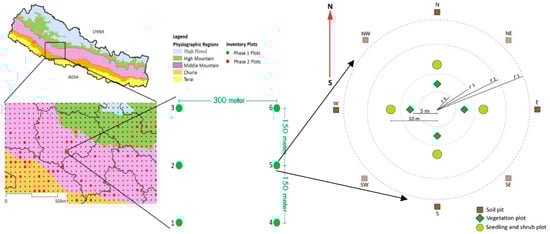
Figure 1.
Data collection from the permanent sample plots (PSPs) during forest resource assessment (2010–2014). Source: DFRS/FRA 2014.
2.3. Above Ground Tree Biomass and Soil Organic Carbon Analysis
The former Department of Forest Research and Survey (now Forest Research and Training Center) in Kathmandu, Nepal, analyzed the samples that were collected on the FRA field plots. The above-ground tree biomass (AGTB) was calculated by summing up the stem biomass and branch biomass (Equation (1))
AGTB = Stem biomass + Branch biomass
Stem biomass was calculated as a product of the volume of the stem [45] and air-dried wood density [46]. Similarly, the branch biomass was calculated using a branch-to-stem ratio that was based on the species type and size of the stem at diameter at breast height [47]. The air-dried wood densities of the tree species ranges from 352 kg/m3 for Trewia nudiflora L. to 960 kg/m3 for Acacia catechu (L.F.) wild. were used.
For SOC analysis, four soil samples of the same horizon of the particular subplots were mixed together. Each subplot had 3 soil samples representing three different soil horizons. The Black wet combustion method [48] was then applied in Department of Forest Research and Survey (DFRS) soil laboratory, Nepal, to analyze soil organic carbon. On the other hand, a dry combustion and LECO CHN Analyzer were used in the Metla Soil Laboratory, Finland, to assure the quality of the laboratory test. Soil organic carbon that was analyzed in the soil laboratory was later estimated on a per hectare basis.
2.4. Variable Selection
The source of SOC is the vegetative matter which is triggered by climatic conditions to decompose it into carbon. Forest variables such as basal area (BA), above-ground tree biomass (AGTB), and crown cover (CC) were utilized. These variables are important to directly describe the vegetative biomass and ultimately help to predict SOC. Similarly, topographical variables such as altitude, slope, and aspect were utilized which are important to describe climatic conditions. Both forest and topographical variables were used as predictor variables of the SOC. Further, multicollinearity among the predictor variables was verified using the variance inflation factor (VIF) function in the “car” package of the R program [49]. VIF > 5 shows the presence of multicollinearity among the variables [50]. We retained all of the predictor variables in our model as they had VIF < 5.
2.5. Data Split
Data analysis was focused on assessing SOC based on topographic (altitude, slope, and aspect) and forest variables (AGTB, basal area (BA), and crown cover). The whole data were split into two sets, i.e., one set of data for developing a model and another set of data for validating the model as an independent dataset. Before splitting the data, a boxplot was used to check the presence of outliers in the data. The outliers were checked for measurement, recording, or lab analysis errors. After error validation, 1032 sub plots from 362 clusters were used for the SOC analysis for ordinary data (non-transformed). For the transformed data, however, 862 PSPs from 311 clusters were used. The transformed data only included PSPs that were located above 250 m altitude as soil sample data below 250 m created non-linearity and heteroscedasticity problems in the linear model. The number of PSPs within clusters ranges from 1 to 6 in lowland and 1 to 4 in highland. The majority of the PSPs representing the highland were spaced 300 m apart and we treated them as independent sample plots for this study. The data were split into two sets i.e., data (80%) for developing models and test data (20%) for data validation. The splitting was done by using the createDataPartition function in the “caret” package [51], which splits data randomly into two different sub-sets with different proportions. All data analyses were done in R software [52].
2.6. Modelling
Pearson’s correlation analysis was performed to determine the relationship of SOC with six predictor variables (altitude, basal area, AGTB, slope, aspect, crown cover) using the cor.test function from the “stat” package in R software [52]. Using the predictor variables, six different models (TM1:TM6) were developed against SOC (transformed SOC data) as a response variable. The predictor variables that were used in the models having higher R2 values indicate better fits of the models. The presence of heteroscedasticity and normality in the residuals of the models were tested using the bptest function (which determines whether the residuals in the linear model are homogenously distributed or not) and the shapiro.test function (which determines whether the residuals in the linear models are normally distributed or not) under “lmtest” and “stat” packages, respectively, in R software [53].
2.7. Data Transformation
The models were tested for the assumptions of simple linear regression, i.e., homoscedasticity (p < 0.05) and normality (p > 0.05). To overcome the problem of rejecting the null hypothesis of the homoscedasticity and normality assumption, the response variable (i.e., SOC) was transformed using the BoxCoxTransformation function under “e1071” package in R software [54] to normalize its distribution and six models were developed. The transformation method is used on a non-normal dependent variable to make it into a normal distribution in which statistical tests can be applied.
2.8. Model Validation
An accuracy assessment of the model was conducted to validate the model prediction by using independent test data that had not been used for model development. The predicted value of the response variable was transformed back and compared with the real value that was obtained from the test data. The mean absolute percentage error (MAPE) was used to determine the error percentage of the models to validate the model’s accuracy. MAPE was calculated using the MAPE function from the “MLmetrics” package in R software [51] (Equation (2)). Lower MAPE values indicate higher accuracy of the models.
where,
- n = number of fitted points
- Oi = Actual value of soil organic carbon
- Fi = predicted value of soil organic carbon
The accuracy (A) of the model was calculated using Equation (3).
where,
A = 1−MAPE
- A
- = Accuracy of the model
3. Results
3.1. Distribution of Variables
Altitude, crown cover, slope, aspect, basal area, and above-ground tree biomass (AGTB) were used as predictor variables to describe the SOC as a response variable. Basic statistics of the variables that were used under study are shown (Table 2). More variability in the variables were seen. This could be due to the sample plots that were recorded throughout the country representing larger climatic, ecological, and altitudinal variations.
Table 2.
Distribution of the predictor and response variables.
3.2. Correlation of Variables
In the correlations and scatterplots of the pairwise combinations of the variables, a strong and linear relationship was found between SOC and altitude (r = 0.76, p < 2.2 × 10⁻¹⁶). The correlation between crown cover and slope has also been found significant with SOC. Similarly, a strong but non-linear relationship was found between basal area and AGTB with SOC (Figure 2).
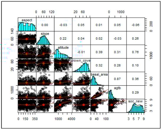
Figure 2.
Pairwise correlations and scatterplots of the seven variables i.e., aspect, slope, altitude, crown cover, basal area, above-ground tree biomass (AGTB), and soil organic carbon.
Moreover, the results also shows that there was a significant correlation (r = 0.87, p < 2.2 × 10⁻¹⁶) between basal area and AGTB which could cause a multi-collinearity problem when both variables are used together in the model.
3.3. Effects of Topography and Stand Level Variables
As untransformed SOC data in the models did not satisfy the assumptions of linear models, the response variable (SOC) was transformed using the Box–Cox transformation method [54] to normalize the regression models. Box and Cox (1964) developed a family of transformations that were designed to reduce the non-normality of the errors in a linear model [55]. In this model, the output of the model (transformed predicted value) needs to be transformed back to get the normal predicted value (Equation (4)).
where,
Normal Predicted value = exp(log(λ × transformed predicted value + 1)/λ)
- Estimated λ = 0.2 (It is an “optimal value” that results in the best approximation of a normal distribution).
Afterward, six different models were developed which fulfilled the assumption of linear regression models (Table 3).
Table 3.
Models after transforming the response variable using the Box–Cox transformation method.
The residuals of the linear model TM6 show random distribution with mean zero (Figure 3a), and normal distribution and homoscedasticity (Figure 3b).
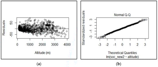
Figure 3.
(a) Distribution of the residuals of the model TM6 showing homogeneity; (b) standardized residuals in the model TM6 showing normality.
All the parameter estimates for each model were significant at the 0.05 level in the transformed model. Among the six predictor variables in the model (TM1), altitude (p < 2 × 10⁻¹⁶), crown cover (p < 0.0011), and slope (p < 0.00015) were significant while aspect, AGTB, and basal area were not significant. Among three significant predictor variables, altitude was found to be more significant. The altitude alone as a predictor in the model (TM6) has a significant effect on the SOC (Table 2).
During the transformation of a response variable, the predictor variable (altitude > 250 m) was used by the hit and trial method. Sample plots that were located below 250 m altitude did not show a significant correlation between altitude and SOC. The inclusion of these samples in the models violated the assumption of the linear model (i.e., heteroscedasticity and non-normality), thus they were excluded in the model development. Finally, for all the transformed models (TM1:TM6), the assumption of linear models was accepted i.e., homoscedasticity (p > 0.05) and normality (p > 0.05). All the candidate models (TM1:TM6) showed similar goodness of fit on the observed data. Better goodness of fit between the observed value and the predicted value of SOC (Figure 4a) and the rate of SOC changes increases with the increase in altitude can be seen (Figure 4b).
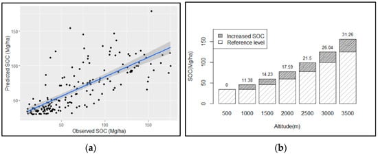
Figure 4.
(a) Observed vs. predicted SOC in the model TM6; (b) SOC changes in the increase of altitude in the model TM6.
The results show that at every increase of 500 m altitude, the SOC increased by 11.38 Mg ha−1 to 31.28 Mg ha−1. Thus, our study confirms that an increase in the SOC amount increases with the increase in altitude (Figure 4b) i.e., the rate of increase of SOC is higher at higher altitudes. Alternatively, the SOC does not increase uniformly with altitude. Instead of proportionality, the change in SOC increases with increasing altitude.
3.4. Accuracy of the Model
Based on the number of predictor variables, TM6—the model with one predictor variable—was found to be an appropriate model for predicting the SOC. Using altitude alone (TM6) provided a similar level of accuracy compared to the other models that used, in addition to altitude, additional predictor variables. In model TM6, the predictor variable altitude was found significant to predict the SOC, producing an accuracy of 67.33% (Table 4).
Table 4.
Accuracy of the models.
Other variables in the model seemed to be dispensable due to the small accuracy gains. Comparing the results of all the models show that altitude alone (TM6) is the most influential variable to predict SOC with simultaneously maintaining sufficient accuracy with respect to the inclusion of other predictor variables (in TM1:TM5).
4. Discussion
4.1. Distribution of SOC
The storage of SOC is influenced by various factors such as climatic, edaphic and biotic factors [56], and topographic factors [57,58]. In this study, the distribution of SOC concentrates more from the lower elevation region towards the higher elevation region (lower region to high mountain region). This is due to higher altitude-induced low-temperature resulting in lower activities of microbes that are involved in SOM decomposition [59,60]. In Nepal, the average temperature decreases by 6 °C for every 1000 m increase in altitude [36]. A lower temperature is likely to control the retention of SOC [20,61] which shows that the decreasing trend of temperature from lower to higher regions is contributing to higher SOC accumulation. Furthermore, the extraction of forest products (litter, branches, timber) from the forest can also influence the accumulation of SOC due to the reduced availability of forest organic material that can be converted to soil organic matter [62]. Forest product extraction depends on the accessibility of the forest. Accessibility to forests at higher altitudes is difficult due to the rugged terrain compared to lower regions. It is supported by the results that forest disturbances by humans (tree cutting, bush cutting, litter collection, lopping, and cattle grazing) are lower at higher altitudes [40]. Therefore, it can be concluded that the distribution of SOC is likely to be concentrated more on the region with less anthropogenic disturbances compared to a region of higher disturbance [63].
4.2. Effect of Topographic and Stand Variables on SOC
The higher variation in SOC in different sites is due to the variation in topographic, climatic factors, and anthropogenic disturbances. Topographical factors are the main factors contributing to the spatial variability of the SOC [64,65,66] and induce heterogeneity in SOC which is likely to produce large uncertainties in SOC storage [67,68]. Our study shows altitude as a major significant variable to predict the SOC followed by slope while aspect is insignificant. Aspect has an influence on the local temperature, therefore, microbial activities could be less important. The positive correlation of SOC with altitude implies a negative correlation of SOC with temperature; as altitude increases, the temperature decreases. The formation of SOC mainly depends on the rate of decomposition that is influenced by the temperature; the lower the temperature, the lesser the control on SOC accumulation [20]. A similar trend that was in line with our finding (i.e., positive correlation of SOC and altitude) has been reported in several studies in different regions. e.g., Meghalaya, India (150–1961 m); Brazilian Atlantic Forest (100–1000 m); Mt. Kilimanjaro, Tanzania (750–4000 m); Southern Appalachian, USA (235–1670 m); Saruwaged Mountain, Papua New Guinea’s (100–3050 m); Moncayo Massif, SW Europe (1000–1600 m); Mt Changbai, China (700–2000 m); Tropical Montane Forest (1000–3600 m); Bale Mountains, Ethiopia (2390–3250 m); Spain (607–1168 m); and Ethiopia (2034–2410 m) [13,27,28,29,30,31,32,69,70,71,72].
Contrastingly, there are also studies showing decreasing stocks of SOC with increasing altitude [15,33] and no significant relationship between SOC and altitude [73]. These studies were conducted within shorter altitudinal ranges (500–1200 m, 1600–2200 m, 1800–2200 m, 2200–2500 m). Due to the underlying short ranges of altitudes, other variables may have more effect on the SOC. [17] studies SOC in the Mawer Range in India for two attitudinal zones (1800–2200 m and 2200–2500 m) and presents that the mean values of SOC are decreasing with increasing altitude. However, when considering the 95% confidence intervals that were presented by [17], the dissimilarity that was presented was not significant. Altitude does not directly affect the ecosystem but is an indicator of climatic functions [37]. The SOC distribution depends on the altitude-induced variation in climatic variables (temperature, precipitation). The forest soil organic carbon stocks increase with altitude due to slow soil organic matter decomposition at the colder higher elevation sites [70,71].
Our study shows a positive relationship of SOC with slope. The maximum slope that was used in the study was 45° (100%). The increasing slope indicates a higher retention of SOC. Similar findings were reported for slope by [69,74,75] and slope aspect [76]. Land surface temperature decreases with the increase of slope by influencing incidence angle and reflectivity of solar radiation [77], hence a lower rate of decomposition contributing to more SOC retention [20]. Contrary to our findings, [78] found an inverse relationship of SOC with the slope which might be due to the study being confined to a steep and narrow catchment, thereby emphasizing erosive down-hill transport of leaf litter and soil debris.
Moreover, unlike our study, [13] presents a significant effect of aspect on SOC. The study was confined to small areas, so the micro-climatic (local effect) might have an effect on the SOC. Similarly, [68] reports that slope and aspect are major variables that affect the distribution of SOC. The study was conducted within a shorter interval of altitudinal range (i.e., 2400–4000 m), thus slope and aspect could have a strong effect on the SOC. Our study shows that aspect does not hold a strong relationship with SOC in the larger altitudinal variations. The weak relationship between aspect and SOC in the forest area with large altitudinal ranges may be due to the large-scale effect that might filter out the effect of micro-climate.
Similarly, our study gives an indication of the effect of different stand variables (above-ground tree biomass, basal area, and crown cover) on the SOC. Crown cover affects SOC more than above-ground tree biomass and basal area. Crown cover has significant positive correlation with SOC. A similar finding has also been reported by [69]. In fact, tree crown cover helps to reduce soil temperature [79,80]. High crown cover lowers the rate of decomposition of organic matter leading to more SOC retention [20] while an increase in the mean annual temperature decreases the amount of SOC [81]. Relationships between the crown cover and temperature, and between temperature and SOC suggest that maintaining continuous crown cover in the forest contributes to higher SOC accumulation.
Our results did not find a correlation between the above-ground tree biomass and basal area with SOC. On the contrary, a negative correlation between tree biomass (above- and below-ground biomass) and SOC was reported in a case study of community forests in Nepal [82]. Similarly, a negative correlation between the basal area and SOC was reported in the tropical forests of Bangladesh [74]. Contrasting results depict that tree biomass and SOC do not follow the same trend, although the above-ground biomasses are the source of SOC. Tree biomass (tree carbon) is mainly affected by human disturbance and stand structure while SOC is primarily affected by local climate [74]. The disproportionate level of anthropogenic disturbance (tree cutting, forest fire, lopping) along the physiographic regions of Nepal [40] might be a reason for AGTB as a weak predictor for SOC. This was similar the basal area and SOC as basal area and the AGTB were strongly correlated (r = 0.86).
4.3. Altitudinal Effect on SOC and Its Implication
Most of the studies show positive relationship between altitude and the SOC [64,71,83]. Our study also confirms the same relationship by analyzing nationwide data representing a wider variation of altitudinal range from 250 to 3993 m. The results hold good only for the altitudinal ranges that were covered with forests as at some point forest productivity declines and affects SOC accumulation due to climate limitations. In addition, our results show a change in the amount of SOC increases with the increase of altitude. A decrease in the temperature with an increase in the altitude [36] that is accompanied by less anthropogenic disturbance to the forest at higher altitudes [40] could be the reason for SOC accumulation at higher rates at higher altitudes.
The developed model using altitude solely as a predictor of SOC produces two thirds of the accuracy of the model. As such, this can be an option to assess the SOC distribution at the national scale. In addition, the present model gives an avenue to use other predictor variables (along with altitude) including other variables to build more robust models for the estimation of SOC in the future. The phenomena of decreasing temperature with increasing altitude suggests that altitude may be taken as a proxy for increasing temperatures in studies examining the influence of future climate change on SOC. Our study provides a basis for studying the effect of changing temperature patterns due to climate change on soil organic carbon.
Globally, soil alone contains more carbon than the atmosphere and vegetation combined [84]. Thus, a small variation in SOC concentrations can significantly affect the global carbon cycle [85]. Higher altitude forests have the highest biomass density and also store a large amount of SOC in Nepal [40]. According to our results, an increasing rate of change in the amount of SOC with an increase in altitude shows that higher altitude forests are more important from a climate change mitigation perspective. They have been contributing to climate change mitigation by acting as a carbon sink, both with trees and forest soil.
The study covers large areas with a higher altitudinal variation. Such a large-scale study has cancelled out the micro-climatic effect which is very important for small areas for the estimation of SOC. Furthermore, human disturbance of the forest has also a relationship with altitude in a country such as Nepal. The disturbance is directly related to the accessibility (road networks) of the forest; when more the forest is accessible, more is likely to be disturbed. Therefore, altitude can be considered as a proxy of temperature along with human disturbance which shows a confounding effect on SOC stock.
5. Conclusions
The study assessing SOC on the basis of crown cover, slope, and altitude has contributed to a better understanding of biophysical factors that potentially affect SOC, in particular altitude. Our study confirms the positive relationship between SOC and altitude. Particularly, the finding of the study suggests that the rate of SOC accumulation increases with the increase in altitude. However, according to the Third National Communication Report of Nepal to UNFCCC, an increase in temperature is at a higher rate at higher altitude [86] which shows a potential increase in carbon emissions from the forest soil at higher altitudes. With these findings, our study highlights the need for sustainable management of high-altitude forests to maximize the mitigation potential of the forest ecosystems protecting fragile landscapes in Nepal.
Moreover, altitude as a single predictor for large and higher altitudinal variation area, predicted with two thirds of the accuracy for SOC estimation and so could be useful in the future estimation of SOC during national level carbon inventory. Similarly, altitude is an index of climatic functions [37], thus it can be used as a proxy of climatic variables (i.e., temperature). Altitude has possible insights into the influence of changing temperature patterns on SOC due to future climate change. Using the relationship between altitude and SOC, future studies focusing on the SOC distribution under different forest types will provide a better understanding of the contribution of the forest types in climate change mitigation through SOC accumulation.
Author Contributions
R.M., P.R.N. and M.K. contributed on designing the study. R.M. contributed on data acquisition, data analysis, and drafting manuscript. P.R.N. and M.K. contributed on drafting to the final stage of the manuscripts. All authors have read and agreed to the published version of the manuscript.
Funding
This research was partially funded by the Deutsche Forschungsgemeinschaft (DFG, German Research Foundation) under Germany’s Excellence Strategy—EXC 2037 ‘CLICCS—Climate, Climatic Change, and Society’—Project Number: 390683824, contribution to the Center for Earth System Research and Sustainability (CEN) of Universität Hamburg, Hamburg, Germany.
Institutional Review Board Statement
Not applicable.
Informed Consent Statement
Not applicable.
Data Availability Statement
Data that supports the findings of this study are available from Forest Research and Training Centre (FRTC), Kathmandu, Nepal but not publicly accessible due to the data sharing protocol of the FRTC. However, data can be obtained by following formal process of written application with supporting documents.
Acknowledgments
The Authors are thankful to FRTC, Kathmandu for the provision of data and to the reviewers for their constructive comments and suggestions.
Conflicts of Interest
The authors declare no conflict of interest.
References
- IPCC. IPCC Good Practice Guidance for Land Use, Land-Use Change and Forestry; IPCC National Greenhouse Gas Inventory Program; Technical Support Unit: Hayama, Kanagawa, 2003. [Google Scholar]
- Neupane, P.R.; Gauli, A.; Maraseni, T.; Kübler, D.; Mundhenk, P.; Dang, M.V.; Kohl, M. A segregated assessment of total carbon stocks by the mode of origin and ecological functions of forests: Implication on restoration potential. Int. For. Rev. 2017, 19, 120–147. [Google Scholar]
- Shi, Y.; Baumann, F.; Ma, Y.; Song, C.; Kühn, P.; Scholten, T.; He, J.-S. Organic and inorganic carbon in the topsoil of the Mongolian and Tibetan grasslands: Pattern, control and implications. Biogeosciences 2012, 9, 2287–2299. [Google Scholar] [CrossRef]
- Song, B.; Niu, S.; Zhang, Z.; Yang, H.; Li, L.; Wan, S. Light and Heavy Fractions of Soil Organic Matter in Response to Climate Warming and Increased Precipitation in a Temperate Steppe. PLoS ONE 2012, 7, e33217. [Google Scholar] [CrossRef] [PubMed]
- Singh, B.K. Soil Carbon Storage: Modulators, Mechanisms and Modeling; Academic Press: Cambridge, MA, USA, 2018. [Google Scholar]
- Sedjo, R.A. The carbon cycle and global forest ecosystem. Water Air Soil Pollut. 1993, 70, 295–307. [Google Scholar] [CrossRef]
- Li, M.; Zhang, X.; Pang, G.; Han, F. The estimation of soil organic carbon distribution and storage in a small catchment area of the Loess Plateau. CATENA 2013, 101, 11–16. [Google Scholar] [CrossRef]
- Thompson, J.A.; Kolka, R.K. Soil Carbon Storage Estimation in a Forested Watershed using Quantitative Soil-Landscape Modeling. Soil Sci. Soc. Am. J. 2005, 69, 1086–1093. [Google Scholar] [CrossRef]
- Ontl, T.; Schulte, L.A. Soil Carbon Storage. Nat. Educ. Knowl. 2012, 3, 35. [Google Scholar]
- Garten, C.T. Soil Carbon Dynamics Along an Elevation Gradient in the Southern Appalachian Mountains; Environment Sciences Division-Oak Ridge National Laboratory: Oak Ridge, TN, USA, 2004.
- Zhu, B.; Wang, X.; Fang, J.; Piao, S.; Shen, H.; Zhao, S.; Peng, C. Altitudinal changes in carbon storage of temperate forests on Mt Changbai, Northeast China. J. Plant Res. 2010, 123, 439–452. [Google Scholar] [CrossRef]
- Yoo, K.; Amundson, R.; Heimsath, A.M.; Dietrich, W.E. Spatial patterns of soil organic carbon on hillslopes: Integrating geomorphic processes and the biological C cycle. Geoderma 2006, 130, 47–65. [Google Scholar] [CrossRef]
- Chaturvedi, S.S.; Sun, K. Soil organic carbon and carbon stock in community forests with varying altitude and slope aspect in Meghalaya, India. Int. Res. J. Environ. Sci. 2018, 7, 1–6. [Google Scholar]
- Jakšić, S.; Ninkov, J.; Milić, S.; Vasin, J.; Živanov, M.; Jakšić, D.; Komlen, V. Influence of Slope Gradient and Aspect on Soil Organic Carbon Content in the Region of Niš, Serbia. Sustainability 2021, 13, 8332. [Google Scholar] [CrossRef]
- Bangroo, S.; Najar, G.; Rasool, A. Effect of altitude and aspect on soil organic carbon and nitrogen stocks in the Himalayan Mawer Forest Range. CATENA 2017, 158, 63–68. [Google Scholar] [CrossRef]
- Mohammad, S.; Rasel, M. Effect of Elevation and Above Ground Biomass (AGB) on Soil Organic Carbon (SOC): A Remote Sensing Based Approach in Chitwan District. Nepal. Int. J. Sci. Eng. Res. 2013, 4, 1546–1553. [Google Scholar]
- Jevon, F.V.; D’Amato, A.W.; Woodall, C.W.; Evans, K.; Ayres, M.P.; Matthes, J.H. Tree basal area and conifer abundance predict soil carbon stocks and concentrations in an actively managed forest of northern New Hampshire, USA. For. Ecol. Manag. 2019, 451, 117534. [Google Scholar] [CrossRef]
- Kara, Ö.; Bolat, I.; Çakiroğlu, K.; Öztürk, M. Plant canopy effects on litter accumulation and soil microbial biomass in two temperate forests. Biol. Fertil. Soils. 2008, 45, 193–198. [Google Scholar] [CrossRef]
- Liu, Y.; Li, S.; Sun, X.; Yu, X. Variations of forest soil organic carbon and its influencing factors in east China. Ann. For. Sci. 2016, 73, 501–511. [Google Scholar] [CrossRef]
- Zinn, Y.L.; Andrade, A.; Araújo, M.A.; Lal, R. Soil organic carbon retention more affected by altitude than texture in a forested mountain range in Brazil. Soil Res. 2018, 56, 284. [Google Scholar] [CrossRef]
- Sah, S.P.; Brumme, R. Altitudinal gradients of natural abundance of stable isotopes of nitrogen and carbon in the needles and soil of a pine forest in Nepal. J. For. Sci. 2018, 49, 19–26. [Google Scholar] [CrossRef]
- Pradhan, B.M.; Awasthi, K.D.; Bajracharya, R.M. Soil organic carbon stocks under different forest types in Pokhare khola sub-watershed: A case study from Dhading district of Nepal. WIT Trans. Ecol. Environ. 2012, 157, 535–546. [Google Scholar] [CrossRef]
- Ghimire, P.; Bhatta, B.; Pokhrel, B.; Kafle, G.; Paudel, P. Soil organic carbon stocks under different land uses in Chure region of Makawanpur district, Nepal. SAARC J. Agric. 2019, 16, 13–23. [Google Scholar] [CrossRef]
- Sharma, M.; Kafle, G. Comparative assessment of profile storage of soil organic carbon and total nitrogen in forest and grassland in Jajarkot, Nepal. J. Agric. Nat. Resour. 2020, 3, 184–192. [Google Scholar] [CrossRef]
- Adhikari, B.M.; Ghimire, P. Assessment of Soil Organic Carbon Stock of Churia Broad Leaved Forest of Nawalpur District, Nepal. Grassroots J. Nat. Resour. 2019, 2, 45–52. [Google Scholar] [CrossRef]
- Bajracharya, R.M.; Sitaula, B.; Shrestha, B.M.; Awasthi, K.D. Soil organic carbon status and dynamics in the central Nepal middle mountains. Forestry 2004, 12, 28–44. [Google Scholar]
- Dalmolin, R.S.D.; Gonçalves, C.N.; Dick, D.P.; Knicker, H.; Klamt, E.; Kögel-Knabner, I. Organic matter characteristics and distribution in Ferralsol profiles of a climosequence in southern Brazil. Eur. J. Soil Sci. 2006, 57, 644–654. [Google Scholar] [CrossRef]
- Sousa Neto, E.; Carmo, J.B.; Keller, M.; Martins, S.C.; Alves, L.F.; Vieira, S.A.; Piccolo, M.D.; Camargo, P.; Couto, H.T.; Joly, C.A.; et al. Soil-atmosphere exchange of nitrous oxide, methane and carbon dioxide in a gradient of elevation in the coastal Brazilian Atlantic forest. Biogeosciences 2011, 8, 733–742. [Google Scholar] [CrossRef] [Green Version]
- Zech, M.; Hörold, C.; Leiber-Sauheitl, K.; Kühnel, A.; Hemp, A.; Zech, W. Buried black soils on the slopes of Mt. Kilimanjaro as a regional carbon storage hotspot. CATENA 2014, 112, 125–130. [Google Scholar] [CrossRef]
- Garten, C.T.; Hanson, P.J. Measured forest soil C stocks and estimated turnover times along an elevation gradient. Geoderma 2006, 136, 342–352. [Google Scholar] [CrossRef]
- Dieleman, W.I.; Venter, M.; Ramachandra, A.; Krockenberger, A.; Bird, M. Soil carbon stocks vary predictably with altitude in tropical forests: Implications for soil carbon storage. Geoderma 2013, 204–205, 59–67. [Google Scholar] [CrossRef]
- Badía, D.; Ruiz, A.; Girona, A.; Martí, C.; Casanova, J.; Ibarra, P.; Zufiaurre, R. The influence of elevation on soil properties and forest litter in the Siliceous Moncayo Massif, SW Europe. J. Mt. Sci. 2016, 13, 2155–2169. [Google Scholar] [CrossRef]
- Sheikh, M.A.; Kumar, M.; Bussmann, R.W. Altitudinal variation in soil organic carbon stock in coniferous subtropical and broadleaf temperate forests in Garhwal Himalaya. Carbon Balance Manag. 2009, 4, 6. [Google Scholar] [CrossRef]
- Liu, N.; Nan, H. Carbon stocks of three secondary coniferous forests along an altitudinal gradient on Loess Plateau in inland China. PLoS ONE 2018, 13, e0196927. [Google Scholar] [CrossRef] [PubMed]
- HMGN/MFSC. Nepal Biodiversity Strategy; HMGN/MFSC: Kathmandu, Nepal, 2002; pp. 1–117. [Google Scholar]
- Jha, P.K. Environment and Man in Nepal; Craftsman Press: Bangkok, Thailand, 1992. [Google Scholar]
- Hanawalt, R.B.; Whittaker, R.H. Altitudinally coordinated patterns of soils and vegetation in the San Jacinto mountains, California. Soil Sci. 1976, 121, 114–124. [Google Scholar] [CrossRef]
- LRMP. Summary Report. Kathmandu; Land Resources Mapping Project: Kathmandu, Nepal, 1986. [Google Scholar]
- Stainton, J.D.A. Forests of Nepal; Taxon. John Murray: London, UK, 1972. [Google Scholar]
- DFRS. State of Nepal’s Forests; Forest Resource Assessment (FRA) Nepal, Department of Forest Research and Survey (DFRS): Kathmandu, Nepal, 2015.
- Jackson, J. Manual of Afforestation in Nepal; Nepal-United Kingdom Forestry Research Project; Forest Survey and Research Officel; Department of Forests: Kathmandu, Nepal, 1994. [Google Scholar]
- DFRS/FRA. Terai Forests of Nepal; Forest Resource Assessment (FRA) Nepal Project, Department of Forest Research and Survey: Kathmandu, Nepal, 2014; p. 160.
- DFRS. Middle Mountains Forests of Nepal; Forest Resource Assessment (FRA), Department of Forest Research and Survey (DFRS): Kathmandu, Nepal, 2015.
- DFRS. High Mountains and High Himal Forests of Nepal; Department of Forest Research and Survey: Kathmandu, Nepal, 2015.
- Sharma, E.; Pukkala, T. Volume Tables for Forest Trees of Nepal; Forest Survey and Statistics Division: Kathmandu, Nepal, 1990.
- Sharma, E.R.; Pukkala, T. Volume Equations and Biomass Prediction of Forest Trees of Nepal; Forest Research and Statistics Division: Kathmandu, Nepal, 1990.
- MPFS. Master Plan for Forestry Sector; Ministry of Forests and Soil Conservation: Kathmandu, Nepal, 1988.
- Walkley, A.; Black, I.A. An examination of the Degtjareff method for determining soil organic matter, and a proposed modification of the chromic acid titration method. Soil Sci. 1934, 37, 29–38. [Google Scholar] [CrossRef]
- Fox, J.; Weisberg, S. An {R} Companion to Applied Regression, 2nd ed.; Thousand Oaks Sage: California, CA, USA, 2011. [Google Scholar]
- Akinwande, M.O.; Dikko, H.G.; Samson, A. Variance Inflation Factor: As a Condition for the Inclusion of Suppressor Variable(s) in Regression Analysis. Open J. Stat. 2015, 5, 754–767. [Google Scholar] [CrossRef]
- Yachen, Y. MLmetrics: Machine LearningEvaluation Metrics. R Package Version 1.1.1. 2016. Available online: https://CRAN.R-project.org/package=MLmetrics (accessed on 4 November 2020).
- R Core Team. R. A Language and Environment for Statistical Computing; R Foundation for Statistical Computing: Vienna, Austria, 2012; Available online: http://www.R-project.org (accessed on 8 September 2020).
- Zeileis, A.; Hothorn, T. Diagnostic Checking in Regression Relationships. R News 2002, 2, 7–10. [Google Scholar]
- Meyer, D.; Dimitriadou, E.; Hornik, K.; Leisch, F.; Meyer, D.; Weingessel, A. e1071: Misc Functions of the Department of Statistics (e1071), TU Wien. R Package Version 1.7-4. 2020. Available online: https://CRAN.R-project.org/package=e1071 (accessed on 10 November 2020).
- Box, G.E.P.; Cox, D.R. An Analysis of Transformations. J. R. Stat. Soc. Ser. B 1964, 26, 211–243. [Google Scholar] [CrossRef]
- Schimel, D.S.; Braswell, B.; Holland, E.A.; McKeown, R.; Ojima, D.S.; Painter, T.H.; Parton, W.J.; Townsend, A.R. Climatic, edaphic, and biotic controls over storage and turnover of carbon in soils. Glob. Biogeochem. Cycles 1994, 8, 279–293. [Google Scholar] [CrossRef]
- Zhu, M.; Feng, Q.; Zhang, M.; Liu, W.; Qin, Y.; Deo, R.C.; Zhang, C. Effects of topography on soil organic carbon stocks in grasslands of a semiarid alpine region, northwestern China. J. Soils Sediments 2018, 19, 1640–1650. [Google Scholar] [CrossRef]
- Patton, N.R.; Lohse, K.A.; Seyfried, M.S.; Godsey, S.E.; Parsons, S.B. Topographic controls of soil organic carbon on soil-mantled landscapes. Sci. Rep. 2019, 9, 6390. [Google Scholar] [CrossRef]
- Garten, C.T., Jr. Relationships among forest soil C isotopic composition, partitioning, and turnover times. Can. J. For. Res. 2006, 36, 2157–2167. [Google Scholar] [CrossRef]
- Deng, L.; Liu, G.-b.; Shangguan, Z. Land-use conversion and changing soil carbon stocks in China’s “Grain-for-Green” Program: A synthesis. Glob. Chang. Biol. 2014, 20, 3544–3556. [Google Scholar] [CrossRef] [PubMed]
- Zhang, Y.; Ai, J.; Sun, Q.; Li, Z.; Hou, L.; Song, L.; Tang, G.; Li, L.; Shao, G. Soil organic carbon and total nitrogen stocks as affected by vegetation types and altitude across the mountainous regions in the Yunnan Province, south-western China. CATENA 2020, 196, 104872. [Google Scholar] [CrossRef]
- Baral, S.K.; Katzensteiner, K. Impact of biomass extraction on soil properties and foliar nitrogen content in a community forest and a semi-protected natural forest in the central mid-hills of Nepal. Trop. Ecol. 2015, 56, 323–333. [Google Scholar]
- Mehta, V.K.; Sullivan, P.J.; Walter, M.T.; Krishnaswamy, J.; DeGloria, S.D. Impacts of disturbance on soil properties in a dry tropical forest in Southern India. Ecohydrology 2008, 1, 161–175. [Google Scholar] [CrossRef]
- Yimer, F.; Ledin, S.; Abdelkadir, A. Soil organic carbon and total nitrogen stocks as affected by topographic aspect and vegetation in the Bale Mountains, Ethiopia. Geoderma 2006, 135, 335–344. [Google Scholar] [CrossRef]
- Lozano-García, B.; Parras-Alcántara, L.; Brevik, E.C. Impact of topographic aspect and vegetation (native and reforested areas) on soil organic carbon and nitrogen budgets in Mediterranean natural areas. Sci. Total Environ. 2016, 544, 963–970. [Google Scholar] [CrossRef]
- Chen, L.-F.; He, Z.-B.; Du, J.; Yang, J.-J.; Zhu, X. Patterns and environmental controls of soil organic carbon and total nitrogen in alpine ecosystems of northwestern China. CATENA 2016, 137, 37–43. [Google Scholar] [CrossRef]
- Hancock, G.; Murphy, D.; Evans, K. Hillslope and catchment scale soil organic carbon concentration: An assessment of the role of geomorphology and soil erosion in an undisturbed environment. Geoderma 2010, 155, 36–45. [Google Scholar] [CrossRef]
- Zhu, M.; Feng, Q.; Qin, Y.; Cao, J.; Li, H.; Zhao, Y. Soil organic carbon as functions of slope aspects and soil depths in a semiarid alpine region of Northwest China. CATENA 2017, 152, 94–102. [Google Scholar] [CrossRef]
- Gebeyehu, G.; Soromessa, T.; Bekele, T.; Teketay, D. Carbon stocks and factors affecting their storage in dry Afromontane forests of Awi Zone, northwestern Ethiopia. J. Ecol. Environ. 2019, 43, 7. [Google Scholar] [CrossRef]
- Schindlbacher, A.; De Gonzalo, C.; Díaz-Pines, E.; Gorría, P.; Matthews, B.; Inclán, R.; Zechmeister-Boltenstern, S.; Rubio, A.; Jandl, R. Temperature sensitivity of forest soil organic matter decomposition along two elevation gradients. J. Geophys. Res. Biogeosciences 2010, 115, G03018. [Google Scholar] [CrossRef]
- Tashi, S.; Singh, B.; Keitel, C.; Adams, M. Soil carbon and nitrogen stocks in forests along an altitudinal gradient in the eastern Himalayas and a meta-analysis of global data. Glob. Chang. Biol. 2016, 22, 2255–2268. [Google Scholar] [CrossRef] [PubMed]
- Parras-Alcántara, L.; Lozano-García, B.; Galán-Espejo, A. Soil organic carbon along an altitudinal gradient in the Despenaperros Natural Park, southern Spain. Solid Earth 2015, 6, 125–134. [Google Scholar] [CrossRef]
- Devi, A.S. Influence of trees and associated variables on soil organic carbon: A review. J. Ecol. Environ. 2021, 45, 5. [Google Scholar] [CrossRef]
- Saimun, M.R.; Karim, R.; Sultana, F.; Arfin-Khan, M.A. Multiple drivers of tree and soil carbon stock in the tropical forest ecosystems of Bangladesh. Trees For. People 2021, 5, 100108. [Google Scholar] [CrossRef]
- Wang, S.; Wang, X.; Ouyang, Z. Effects of land use, climate, topography and soil properties on regional soil organic carbon and total nitrogen in the Upstream Watershed of Miyun Reservoir, North China. J. Environ. Sci. 2012, 24, 387–395. [Google Scholar] [CrossRef]
- Liu, M.; Yu, R.; Li, L.; Xu, L.; Mu, R.; Zhang, G. Distribution Characteristics of SOC, STN, and STP Contents Along a Slope Aspect Gradient of Loess Plateau in China. Front. Soil Sci. 2021, 1, 1–12. [Google Scholar] [CrossRef]
- Peng, X.; Wu, W.; Zheng, Y.; Sun, J.; Hu, T.; Wang, P. Correlation analysis of land surface temperature and topographic elements in Hangzhou, China. Sci. Rep. 2020, 10, 10451. [Google Scholar] [CrossRef]
- Kobler, J.; Zehetgruber, B.; Dirnböck, T.; Jandl, R.; Mirtl, M.; Schindlbacher, A. Effects of aspect and altitude on carbon cycling processes in a temperate mountain forest catchment. Landsc. Ecol. 2019, 34, 325–340. [Google Scholar] [CrossRef]
- Lozano-Parra, J.; Pulido, M.; Lozano-Fondón, C.; Schnabel, S. How do soil moisture and vegetation covers influence soil temperature in drylands of Mediterranean regions? Water 2018, 10, 1747. [Google Scholar] [CrossRef]
- Agena, A. Effects of three tree species on microclimate and soil amelioration in the central rift valley of Ethiopia. J. Soil Sci Environ. Manag. 2014, 5, 62–71. [Google Scholar]
- Fissore, C.; Giardin, C.P.; Kolka, R.K.; Trettin, C.C.; King, G.M.; Jurgensen, M.F.; Barton, C.D.; Mcdowell, S.D. Temperature and vegetation effects on soil organic carbon quality along a forested mean annual temperature gradient in North America. Glob. Chang. Biol. 2008, 14, 193–205. [Google Scholar] [CrossRef]
- Pandey, H.P.; Pandey, P.; Pokhrel, S.; Mandal, R.A. Relationship between soil properties and forests carbon: Case of three community forests from Far Western Nepal. Banko Janakari 2019, 29, 43–52. [Google Scholar] [CrossRef]
- Labaz, B.; Galka, B.; Bogacz, A.; Waroszewski, J.; Kabala, C. Factors influencing humus forms and forest litter properties in the mid-mountains under temperate climate of southwestern Poland. Geoderma 2014, 230–231, 265–273. [Google Scholar] [CrossRef]
- FAO; ITPS. Status of the World’s Soil Resources (SWSR)—Main Report; Intergovernmental Technical Panel on Soils: Rome, Italy, 2015. [Google Scholar]
- Walter, K.; Don, A.; Tiemeyer, B.; Freibauer, A. Determining Soil Bulk Density for Carbon Stock Calculations: A Systematic Method Comparison. Soil Sci. Soc. Am. J. 2016, 80, 579–591. [Google Scholar] [CrossRef] [Green Version]
- GoN/MoFE. NepalsThird National Communication to the United Nations Framework Convention on Climate Change; Ministry of Forests and Environment: Kathmandu, Nepal, 2021.
Publisher’s Note: MDPI stays neutral with regard to jurisdictional claims in published maps and institutional affiliations. |
© 2022 by the authors. Licensee MDPI, Basel, Switzerland. This article is an open access article distributed under the terms and conditions of the Creative Commons Attribution (CC BY) license (https://creativecommons.org/licenses/by/4.0/).