Article

δ15N in Birch and Pine Leaves in the Vicinity of a Large Copper Smelter Indicating a Change in the Conditions of Their Soil Nutrition

1
Institute of Plant and Animal Ecology UB RAS, 620144 Yekaterinburg, Russia
2
Ilmensky State Reserve, Federal State Budgetary Institution of Science South Urals Research Center of Mineralogy and Geo-Ecology UB RAS, 456317 Miass, Russia
3
Department of Technical Mechanics and Natural Sciences, South Ural State University, 454080 Chelyabinsk, Russia
4
Institute of Fundamental Education, Ural Federal University named after the first President of Russia B.N. Yeltsin, 620002 Yekaterinburg, Russia
*
Author to whom correspondence should be addressed.
Forests 2022, 13(8), 1299; https://doi.org/10.3390/f13081299
Submission received: 25 May 2022 / Revised: 8 August 2022 / Accepted: 11 August 2022 / Published: 15 August 2022
(This article belongs to the Special Issue Stable Isotopes in Dendroecology)

Abstract

:
δ13C and δ15N were analyzed in the leaves of Pinus sylvestris L. and Betula spp. under the conditions of severe heavy metal (Zn, Cu, Cd, and Pb) contamination. Twenty-seven plots located near the Karabash copper smelter (Russia) were studied. No reliable correlation of 13C in tree leaves with the level of pollution was observed. δ15N, both in Pinus sylvestris and Betula spp., increased similarly in polluted areas. δ15N was increased by 2.3‰ in the needles of Pinus sylvestris and by 1.6‰ in the leaves of Betula spp. in polluted plots compared to the background ones. The probable reasons for the increase in δ15N were estimated using multiple regression. The regression model, which includes two predictors: δ15N in the humus horizon and the occurrence of roots in the litter, explains 33% of the total variability of δ15N in leaves. Thus, in ecosystems polluted with heavy metals, the state of trees is determined not only by the direct toxic effects of heavy metals but also by indirect ones associated with the features of plant mineral nutrition. This fact opens the way to the search for opportunities to control the state of plants in disturbed ecosystems by regulating the content of mineral nutrition elements.

1. Introduction

The stable isotopic ratios of carbon 13C/12C and nitrogen 15N/14N in living organisms and other components of ecosystems are indicators (tracers) of many physiological and environmental processes [1,2,3,4,5]. The δ13C in plants is determined by the nature of their photosynthesis, the life span of leaves, the canopy structure of photosynthetic organs, and environmental conditions [2,3,6,7]. The value of δ15N reflects the 15N content in soil, the diversity of nitrogen sources and the ability of symbiotic nitrogen fixation, as well as the presence of other symbioses [8,9,10]. The differences in plant species and functional groups in terms of δ15N can indicate the general level of nitrogen supply of ecosystems, as well as the degree of its availability and the competition for it [11,12,13,14]. Since the isotopic composition of nitrogen reflects the changes in edaphic conditions in ecosystems as a whole [4], its analysis is used in the study of ecosystems processes [13,15,16,17], including successions [18,19].
Under the conditions of anthropogenic impact, δ13C and δ15N in plants change in different ways. For example, δ13C in tree rings might be increased [4,20,21] or decreased [22,23,24] during pollution. Recently, an increase in δ13C in plant leaves near a large metallurgical smelter was demonstrated [25]. The δ15N may also be increased [26,27,28,29] and decreased [23,24] during urbanization and under the influence of gaseous pollutants. In forest habitats polluted with heavy metals, δ15N in plants increases [25]. Despite the majority of published results revealing that δ13C and δ15N increase under anthropogenic impacts, it is still difficult to draw unambiguous conclusions. This can be explained by a wide variety of combinations of different types of impacts, geographical and landscape conditions, and taxonomic and functional specifics of plants. This indicates the need for the further accumulation of data on the features of δ13C and δ15N distribution in plants under anthropogenic impacts.
Previously, a unidirectional increase in the content of 15N isotope in the plants of several functional groups near a large metallurgical smelter in the taiga zone of Eurasia was established [30,31]. Nevertheless, the changes in δ13C in plants have not been observed with an increase in heavy metal pollution. The difference in δ15N values between uncontaminated and polluted forests in the leaves of plants of the same functional groups, ectomycorrhizal, with ericoid and arbuscular mycorrhiza is about 2–3.5‰. This is comparable to the differences in δ15N between different soil horizons [12,32] or between plants having different methods of soil nutrition [8]. Thus, the changes in δ15N under heavy metal pollution were found to be significant. This result suggests that pollution is either accompanied by a change in nitrogen sources for plants or nitrogen uptake mechanisms by plants.
However, our past materials [30,31] were only partly reliable due to some methodological features. The δ13C and δ15N measurements from 10 plots were available. The plots were unevenly distributed along the heavy metal pollution gradient. Eight sites were located in the zone of severe pollution and only two in forests with a background level of pollution. Previously, no comparison between δ13C and δ15N in plants and soils was made. In this paper, the main conclusions obtained earlier in the study of δ13C and δ15N across the gradient of strong anthropogenic pollution are verified, and some assumptions about the reasons for the change in δ15N considered as possible hypotheses are tested. As opposed to our first research cycle [31,32], the present work is limited to the analysis of the reactions of trees only.
The aim of the present work is to analyze the changes in the composition of stable carbon and nitrogen isotopes in trees under the conditions of strong transformation of natural ecosystems by the emissions from a large copper smelter in the Southern Urals. Based on published information and our own early materials [30,31], three working hypotheses are formulated and tested. The first hypothesis is that under the conditions of heavy metal contamination, the content of heavy 15N and, possibly, 13C isotopes increase in tree leaves. The second and third hypotheses are assumptions about the possible mechanisms for changing δ15N. The second hypothesis is that the change in δ15N in the trees across the pollution gradient reflects the change in δ15N in soils. The third hypothesis suggests that the change in δ15N in trees across the pollution gradient is associated with deeper rooting in the habitats with higher concentrations of heavy metals in soil.

2. Materials and Methods

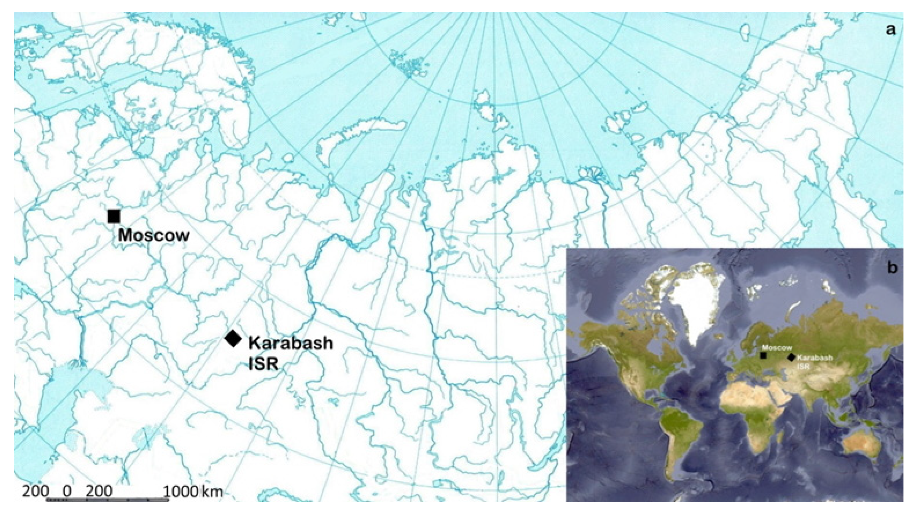
2.1. The Area and Source of Anthropogenic Impact

The study was carried out in the area affected by the industrial emissions from the Karabash copper smelter (KCS) and in the Ilmensky State Reserve (ISR) in the Chelyabinsk region, Southern Urals (Figure 1). The area is situated in the subzone of southern taiga pine-birch forests of the eastern macroslope of the Southern Urals (the Chelyabinsk region in the vicinity of the Karabash and Miass towns). The typical heights of the uplands are 250–600 m a.s.l. Brown mountain-forest and forest, gleyed podzolic, gray mountain-forest, mountain-forest chernozems, and mountain-podzolic shallow soils are represented. The climate is continental and moderately cold. The coldest month is January (average monthly temperature is between –16 and –17 °C), the warmest month is July (+18 °C); the duration of the growing season is 160–170 days from April to September; the rainfall is about 430 mm per year; the snow cover height is up to 40 cm.
The prevailing types of vegetation are forb pine forests and secondary grass-forb birch forests. Regular ground-level vegetation species in the ISR in the absence of pollution are Vaccinium vitis-idaea L., Vaccinium myrtillus L., Calamagrostis arundinacea (L.) Roth, and Rubus saxatilis L. The moss cover is dominated by Pleurozium schreberi (Willd. ex Brid.) Mitt., Rhytidiadelphus triquertus (Hedw.) Warnst., Climacium dendroides (Hedw.) F.Weber & D.Mohr, and Hylocomium splendens (Hedw.) Bruch et al. Soil coverage by mosses in the ISR ranges from 50 to 100% of the soil surface with an average of 70–80%.
The ecosystems of the region are strongly anthropogenically transformed due to various contaminating impacts, including industrial pollution. The Karabash copper smelter (KCS, JSC Karabashmed, Karabash) is a major source of anthropogenic emissions. The main emission components are SO2 and the dust of heavy metals (Cu, Zn, Pb, and Cd). Copper production started in Karabash in 1910, and the largest emissions (up to 140–360 thousand tons per year) were achieved in 1970–1980 [33]. In the period of 1989–1997, copper production stopped, and after the re-opening and modernization of production, the emissions decreased to about 10 thousand tons per year [34,35]. Due to the severe accumulated anthropogenic pollution in the territories closest to the smelter, the zonal ecosystems were completely destroyed: vegetation and the upper parts of the original soils are absent, and a vast anthropogenic wasteland has formed. The levels of accumulation of heavy metals emitted by the KCS in the two-year-old needles of Pinus sylvestris L. are: Cu 8–18 μg/g; Zn 70–150 μg/g; and Pb 30–105 μg/g in the impact zone of the KCS; Cu 2–3 μg/g; Zn 40–45 μg/g, and Pb 1.5–3 μg/g in the Ilmensky State Reserve [36,37]. Due to the accumulation of toxicants, plant damage occurs [33,38] and their diversity decreases [39]. The most stable species of ground-level vegetation are Vaccinium myrtillus L., Calamagrostis arundinacea (L.) Roth, Adenophora lilifolia (L.) A. DC., Lathyrus pisiformis L., Orthilia secunda (L.) House, Sanguisorba officinalis L., Vicia cracca L., and Vicia sylvatica L. The mossy groundcover near the smelter has been fully destroyed, and the ground mosses are missing.

2.2. Sample Plots

The material (leaf samples from five trees, samples of forest litter (A0 horizon) and of the soil mineral part (A1 horizon)) was collected on 27 sample plots. Fifteen areas were located at distances of 5.5–6.5 km in the northeast and south directions from the KCS (impact zone); twelve areas were located 33–50 km south of the KCS (the Ilmensky State Reserve (ISR), background zone) in pine, birch, and mixed pine-birch forests (Table 1). The areas were selected on the middle parts of the slopes on mountain fragmentary and mountain-forest brown incompletely developed soils. The criteria for selecting sample plots were as follows: (1) the forest stands must be of natural origin, i.e., not planted; (2) the age of the main generation of trees must be is close to 100 years or more; and (3) severe or recent anthropogenic disturbances such as logging and soil disturbance must be absent.

2.3. The Determination of Cu, Zn, Pb, and Cd in Litter

The concentrations of Cu, Zn, Pb, and Cd were measured in sample weights taken from the mixed samples of forest litter (A0). Quality control of the analytical procedure was performed by the analysis of the national certified reference materials (CRM). The metals were extracted from soils using nitric acid with a molar concentration of 5 mol/dm3. The ratio of the soil sample weight and acid was 1:5. The quantitative characterization of metals was carried out by ICP-MS on an Agilent 7700X inductively coupled plasma mass spectrometer according to the certified analytical methodology (GOST R 56219-2014). The measurements were performed at a certified laboratory (accreditation certificate No. AAC.A.00330 at the time of measurements; valid until 07/31/2020).
The degree of pollution of each sample plot was characterized by the “litter pollution index”:
Litter   pollution   index = 1 4 ×   C i C min
where Ci and Cmin are the concentrations of one of the four metals (Cu, Zn, Pb, or Cd) in the litter at a certain sample plot (Ci) and minimal in the entire studied range (Cmin). The litter pollution index shows how many times the measured four metals are greater compared to the least contaminated plot. The litter pollution index natural logarithm (litter pollution index (Ln)) of this value was used for the calculations.

2.4. Litter Thickness and Root Occurrence in the Litter

In the summer (July–first half of August) of 2017, 20 measurements of the forest litter thickness were performed on each sample plot. The measurements were carried out one by one in 20 pits randomly placed across the sample plot. The thickness of the enzymatic layer of the forest litter was recorded with an accuracy of 0.5 cm. The presence or absence of roots of any plants in the litter was recorded in a plot with a 20 × 20 cm area at 20 random points.

2.5. The Collection of Leaves, Litter and Soil to Determine δ13C and δ15N

The leaves of 3–5 individuals of two tree taxa, Pinus sylvestris or Betula spp., were collected for isotopic analysis across each sample plot in the summer of 2017 (July–first half of August). Across the three sample plots, only Betula spp. leaves were selected. There were two taxonomically and ecologically similar species of birch in the region that were difficult to distinguish during mass surveys: Betula pendula and Betula pubescens. We did not differentiate these species during leaf collection. On each plot were separately collected P. sylvestris leaves (leaves from five separate P. sylvestris individuals growing on the sample plot were combined into one sample) and Betula spp. leaves (leaves from five separate Betula spp. individuals were combined into one sample). Moreover, for each plot, using the envelope method, one sample of the litter enzymatic horizon and one sample of the upper layer of the soil mineral part were taken, 3–5 cm below the litter boundary.
The samples were dried first in the shade to an air-dry state, then for 48 h at 70 °C in the laboratory’s drying cabinet.
In total, 105 samples were analyzed: 51 samples of tree leaves (24 Pinus sylvestris—1 sample from each of 24 sample plots; 27 Betula spp.—1 sample from each of the 27 sample plots), 27 samples of litter (1 sample from each of the 27 sample plots), and 27 samples of soil mineral parts (1 sample from each of the 27 sample plots).

2.6. Isotopic Analyses

The determination of δ13C and δ15N was carried out at the “Geonauka” Center for Collective Use of the Institute of Geology, Komi Research Center, Ural Branch, Russian Academy of Sciences. Measurements were made using a helium continuous flow mass spectrometry (CF-IRMS) on an analytical complex, including a Flash EA 1112 elemental analyzer connected via a ConFlo IV gas interface to a Delta V Advantage mass spectrometer (Thermo Fisher Scientific, USA). The isotopic composition of nitrogen and carbon were reported per mil relative to the international V-PDB and AIR atmospheric nitrogen standards, δ (‰):
δ Xsample = ((Rsample/Rstandard) − 1) ×1000,
where X is the element (nitrogen or carbon) and R is the molar ratio of the heavy and light isotopes of the corresponding element. The mass spectrometer was calibrated using the USGS-40 (L-Glutamic acid) international standard and the Acetanilide (C8H9NO) in-house standard. The measurement error was ±0.15‰. The measured δ13C and δ15N values in leaves, litter, and soil are given in the Supplementary Materials.

2.7. Data Analysis

Statistical analysis was performed using the JMP 10.0.0 software (SAS Institute Inc., Cary, NC, USA, 2012). The differences in δ13C and δ15N due to the influence of various factors were evaluated by calculating regressions (simple and multiple) and correlations (Pearson’s correlation coefficient (r)). Generalized linear models (GLM) with categorical and continuum predictors were used as well. The combinations of predictors that optimally explained δ15N in plant leaves were selected using the corrected Akaike’s information criterion (AICc) [40]. The values of δ13C and δ15N in each sample of soil, litter, or plant leaves of one taxon on each sample plot or the value of another feature on a sample plot were the units for statistical analysis. The measurement of variability was the standard error (±SE).

3. Results

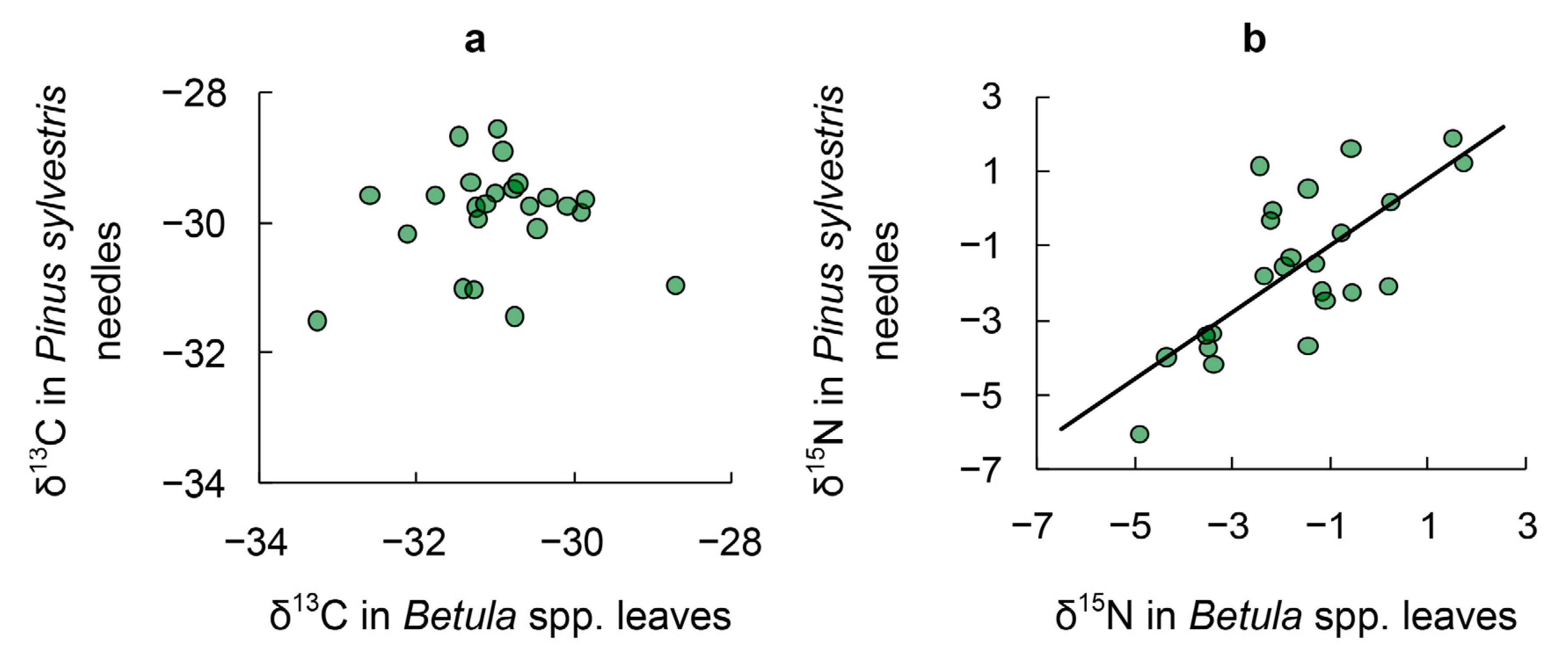
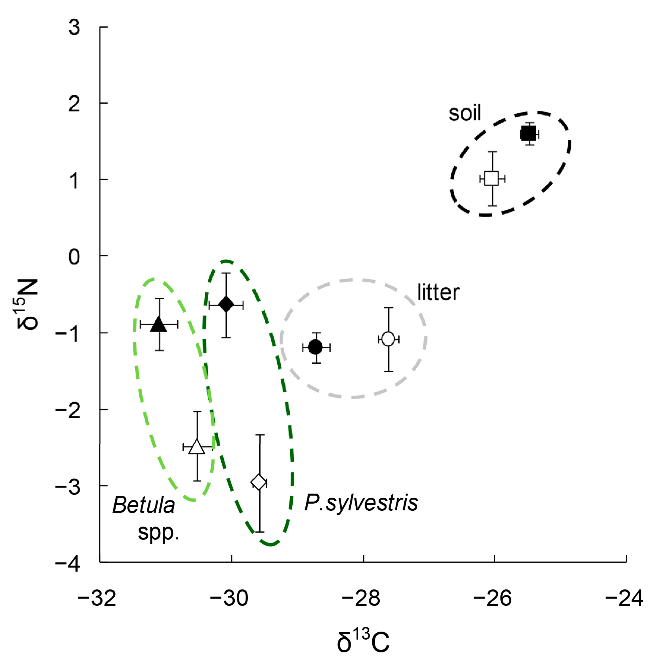
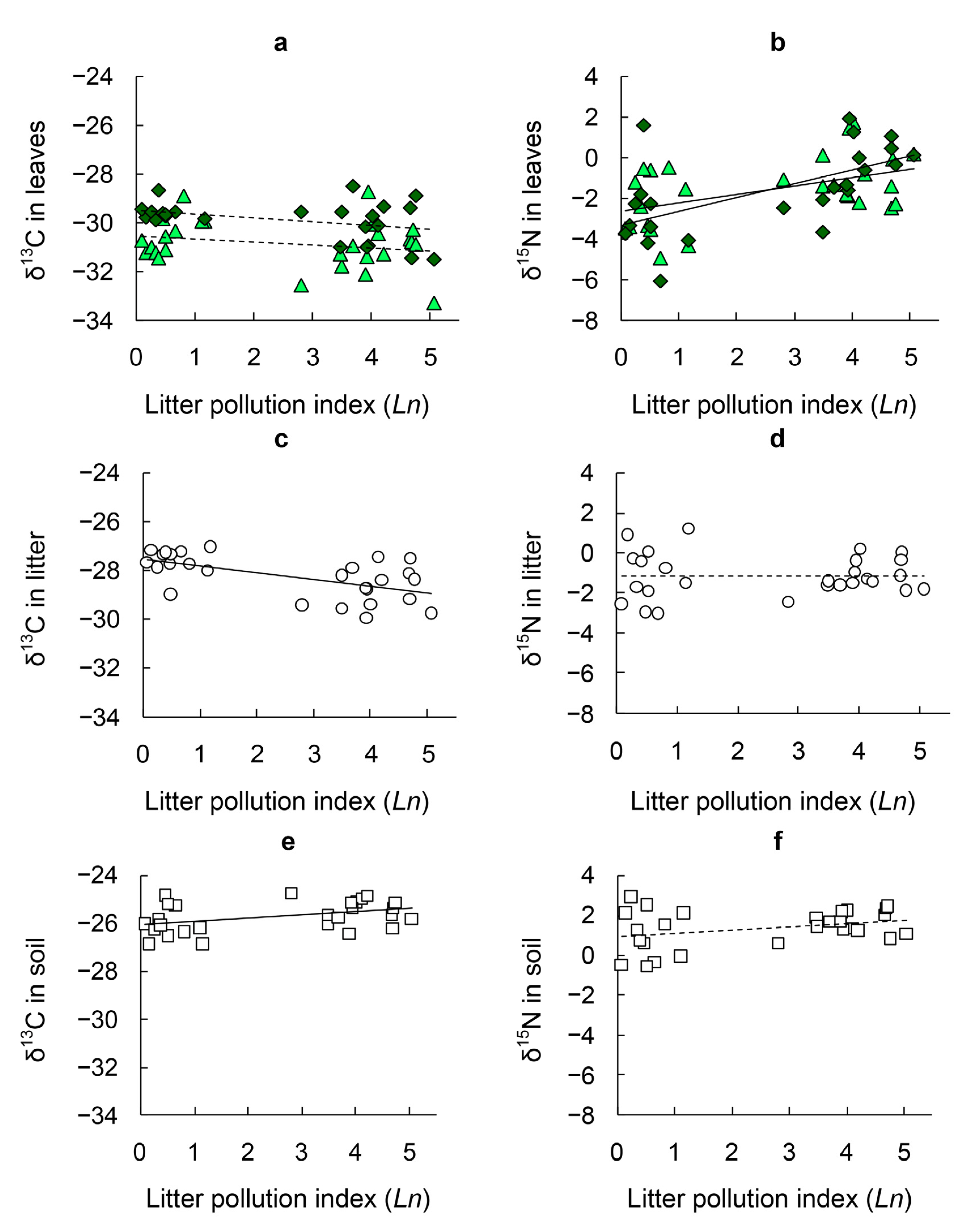
3.1. δ13C in Tree Leaves

The lowest values of δ13C were observed in the leaves of Betula spp. (Figure 2). In Betula spp. Leaves, the average δ13C was equal to −30.85 ± 0.19‰, and for the needles of P. sylvestris δ13C, it was −29.88 ± 0.16‰. These differences were significant in the GLM with the “taxon” and “litter pollution index” factors: Ftaxon = 12.09; p = 0.0003 (Figure 3a). The level of anthropogenic pollution affected the content of 13C in leaves on the boundary of statistical significance (Fpollution = 3.22; p = 0.0479). The average values of δ13C in the absence of pollution were δ13C = −30.10 ± 0.16‰, and near the smelter δ13C = −30.62 ± 0.21‰. Thus, the differences between tree species in δ13C were noticeably larger (the differences were 0.95–1.02‰) than the differences determined by the level of pollution (0.51–0.58‰). The δ13C in Betula spp. leaves and in P. sylvestris needles in different plots did not correlate with each other (Figure 4a): r = 0.09; n = 24; p = 0.6595.

3.2. δ15N in Tree Leaves

The lowest values of δ15N were found in some samples of pine needles (Figure 2), but the differences between Betula spp. and P. sylvestris were not significant. In the GLM with the “taxon” and “litter pollution index” factors Ftaxon = 0.01; p = 0.9469. Depending on the level of pollution, δ15N changed significantly (Fpollution = 20.56; p < 0.0001). The content of the heavy nitrogen isotope in both tree species near the smelter was higher than in the absence of pollution: in Betula spp. by 1.60‰, and in P. sylvestris by 2.33‰ (Figure 3b). The δ15N in Betula spp. leaves and in P. sylvestris needles in different plots significantly correlated with each other (Figure 4b): r = 0.72; n = 24; p < 0.0001.

3.3. δ13C in Litter and Soil

A similar increase in δ13C was observed in a row “tree leaves–litter–humus soil horizon”, both at the background level of pollution and near the smelter. In the ISR forests, the average δ13C values were: −27.63 ±0.15‰ in litter, and −26.05 ± 0.19‰ in the humus soil horizon. In the forests near the copper smelter, the average δ13C values were: −28.73 ± 0.21‰ in litter, and −25.48 ± 0.13‰ in the humus soil horizon. The increase in δ13C during the transition from the leaves to the litter was 2–2.5‰, and 1.5–3‰ during the transition from the litter to soil. Depending on the level of contamination, significant changes in the content of 13C were observed both in litter (Figure 3c) and in soil (Figure 3e). As the pollution increased, the amount of δ13C in the litter decreased. The correlation between the pollution index and δ13C in this horizon was r = −0.58 (p = 0.0015). A similar correlation in the humus horizon was opposite in sign: r = 0.40; p = 0.0411. Consequently, δ13C in the soil increased with increasing pollution.

3.4. δ15N in Litter and Soil

In uncontaminated ISR forests, an increase in δ15N was found in a row “leaves (−2.70 ± 0.37‰)—litter (−1.08 ± 0.41‰)—humus soil horizon (1.02 ± 0.35‰)”. Near the smelter, the content of 15N in leaves (−0.76 ± 0.26‰) and in the litter (−1.19 ± 0.19‰) did not differ statistically. However, from the litter to the soil near the smelter, an increase in δ15N was observed up to a value of δ15N = 1.60 ± 0.14‰, i.e., by almost 3‰. Depending on the level of contamination with heavy metals, the content of 15N (Figure 3d,f) did not change significantly in the litter (r = 0.01; p = 0.9693) or in the humus horizon (r = 0.32; p = 0.0987).

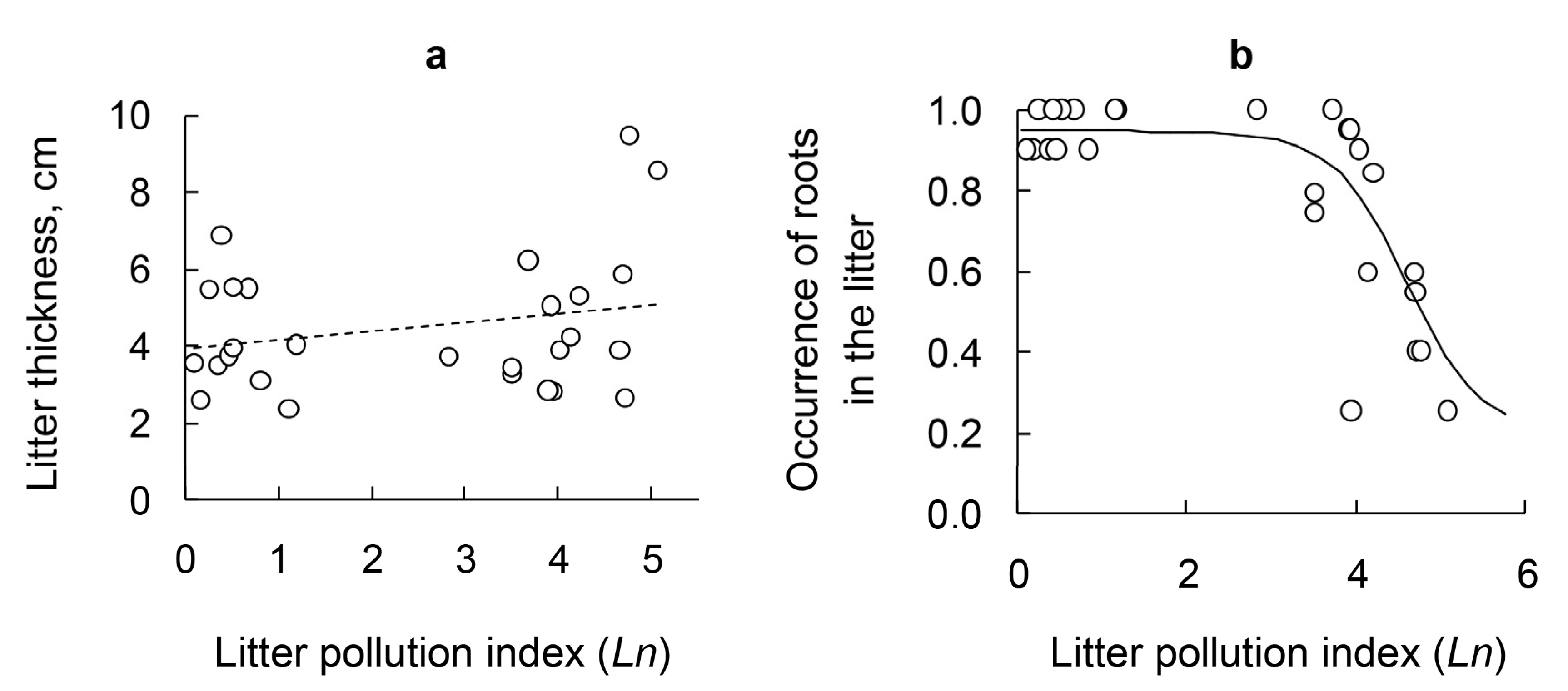
3.5. Litter Thickness and Occurrence of Roots in the Litter

We did not observe an increase in the thickness of the litter layer in the vicinity of KCS (Figure 5a). The correlation coefficient between the litter thickness and the index of its contamination was r = 0.25 (p = 0.2126). However, another noticeable consequence of heavy metal contamination was the disappearance of roots from the litter near the KCS (Figure 5b). The occurrence of roots in relation to the degree of litter contamination was better described by a logistic approximation (R2 = 0.57) rather than by a linear approximation (R2 = 0.46). Consequently, the occurrence of roots in the litter was non-linearly related to the degree of contamination.

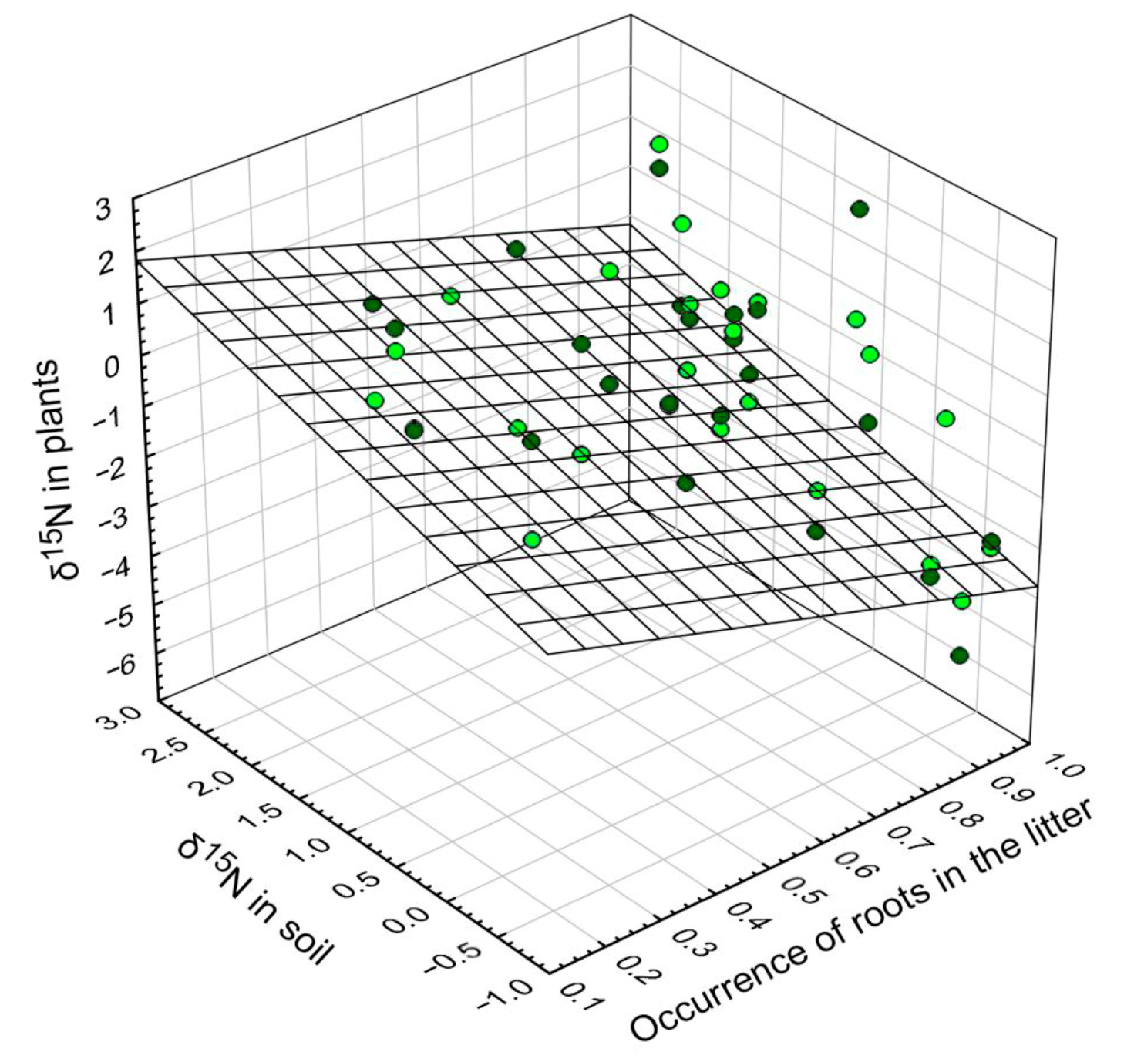
3.6. δ15. N in Tree Leaves versus δ15N in Soil and Root Depth

We suggest that the dynamics of δ15N in tree leaves in the pollution gradient are associated with a change in one of two or both of the following characteristics: the content of δ15N in soils and/or the depth of the root distribution. We first tested these assumptions by evaluating three GLM models. In each model, one of the factors described some property of the habitat, and the second factor was the taxon of the tree—Betula spp. or P. sylvestris. In all three cases, the “taxon” factor and the interaction with its participation were statistically insignificant. The GLM results with the “taxon” and “δ15N in litter” factors: R2 = 0.09; Ftaxon = 0.001 (p = 0.9853); F 15N litter = 4.57 (p = 0.0377); Finteraction = 0.14 (p = 0.7073). The GLM results with the “taxon” and “δ15N in soil” factors: R2 = 0.14; Ftaxon = 0.001 (p = 0.9780); F15N soil = 7.45 (p = 0.0089); Finteraction = 0.02 (p = 0.8960). The GLM results with the “taxon” and “occurrence of roots in the litter” factors: R2 = 0.25; Ftaxon = 0.001 (p = 0.9761); Foccurrence of roots in the litter = 14.70 (p = 0.0004); Finteraction = 1.52 (p = 0.2239). The parameters “δ15N in soil” and “occurrence of roots in the litter” did not correlate with each other (r = –0.11; p = 0.4602). Therefore, they were used as independent predictors in multiple regression. The “taxon” factor did not affect δ15N in leaves. Therefore, to describe δ15N in leaves depending on δ15N in soil and on the depth of the roots, a two-factor regression was used:
δ15Nleaves = 0.231 − 3.348 × occurrence of roots in the litter + 0.643 × δ15Nsoil.
The same expression in a standardized form with beta coefficients:
δ15Nleaves = −0.444 × occurrence of roots in the litter + 0.323 × δ15Nsoil.
Thus, δ15N in leaves depended more strongly on the occurrence of roots in the litter than on δ15N in the soil (Figure 6). The significance of the coefficients was as follows: with the predictor of the occurrence of roots in the litter, p = 0.0005; with the predictor of δ15Nsoil, p = 0.0091. Two predictors explained one third of the variability in δ15N in leaves (R2 = 0.33).

3.7. Other Possible Explanations for δ15N in Tree Leaves

Based on the AICc values, the combination of “δ15N in soil” and “occurrence of roots in the litter” predictors was not optimal for explaining δ15N in tree leaves (Table 2). The best combination of predictors to explain δ15N in leaves was the combination of δ13C and δ15N in litter. The combination of these predictors made it possible to improve the quality of explanation of δ15N variability in tree leaves by 10% compared to the model considered in the previous section. The multiple two-factor regression equation was:
δ15Nleaves = −34.945 − 1.203 × δ13Clitter + 0.537 × δ15Nlitter.
The same expression in a standardized form with beta coefficients:
δ15Nleaves = −0.584 × δ13Clitter + 0.322 × δ15Nlitter.
Based on the AICc values, it was also evident that the degree of litter contamination with heavy metals could be a component of models that satisfactorily explained the variability of δ15N in leaves.

4. Discussion

Higher δ13C values were found in the evergreen needles of P. sylvestris compared to the leaves of deciduous birches. A similar result previously demonstrated by [25] was associated with the peculiarities of stomatal conductance in the leaves of evergreen and deciduous plants. A working hypothesis was formulated about the possible increase in δ13C under pollution conditions, firstly, taking into consideration the predominance of similar results among published works [4,20,21], and secondly, based on the results of a recent study by [25], which was methodologically very close to our work. An increase in δ13C in the leaves of boreal plants in the vicinity of the Ni–Cu smelter was demonstrated [25]. However, the hypothesis about δ13C increase in leaves during the contamination with heavy metals was not confirmed. On the contrary, a slight decrease in δ13C was observed when approaching the smelter. That fact corresponded neither to most of the published data nor to our earlier result, also obtained in the vicinity of the KCS [31].
The conclusion about the decrease in δ13C in trees under polluted conditions does not seem reliable to us for two reasons. First, when we analyzed δ13C separately in the leaves of P. sylvestris and Betula spp., we did not observe a statistically significant decrease in δ13C (which is demonstrated in Figure 3a by dashed lines). Secondly, we did not observe the consistency of the δ13C content in the leaves of P. sylvestris and Betula spp. (see Figure 4a). Therefore, it is highly probable that the content of the 13C isotope in the leaves of trees in our study was due not to the level of contamination of the territory but to some other reasons that we did not evaluate.
Among the most often discussed environmental mechanisms of δ13C variability in plants are the factors regulating the operation of the stomatal apparatus such as the effect of gaseous pollutants [4,23] or moisture level [6]. The emissions from the Karabash smelter during our study were 10–30 times lower than during the highest emissions observed in the mid-1980s [35]. At the same time, even our most polluted areas are 5–7 km away from the source of emissions. There are no forests closer to the smelter that meet the criteria for inclusion in the study. This is due to the influence of high soil toxicity accumulated in the previous period [36,37]. We are not familiar with the data on current levels of air pollution at the studied plots. However, the established slight changes in δ13C across the pollution gradient in the leaves may indicate the absence of strong effects caused by the influence of gaseous pollutants on trees.
We found that δ13C in litter as well as δ13C in leaves decreases across the pollution gradient. However, such a decrease in δ13C in the litter is more pronounced than in the leaves. As a result, the difference between the carbon isotope signature in leaves and in litter decreases across the pollution gradient. In background forests, this difference is 2.91 ± 0.29‰ for Betula spp. and 2.01 ± 0.20% in P. sylvestris, while in the vicinity of KCS it is 2.38 ± 0.33 and 1.40 ± 0.31‰, respectively. Usually, an increase in δ13C from leaves to litter and further to soil is associated with the process of litter microbiological transformation [11,41]. Therefore, a decrease in the difference between δ13C in leaves and litter near the smelter may be an indicator of a slowdown in the process of litter destruction under the conditions of heavy metal pollution. The decrease in the rate of litter degradation under the influence of heavy metals is well documented [42,43]. The plausible mechanism for this is a strong inhibition of destructor organisms under the influence of heavy metal pollution [44,45,46].
We observed the same increase in δ15N in P. sylvestris needles and Betula spp. leaves with increasing heavy metal pollution. This result confirmed our first working hypothesis and our previous results [30,31]. The conclusion about the increase in the 15N heavy isotope in the tree leaves in contaminated areas was also previously made in the vicinity of another metallurgical plant with a similar emission pattern [25]. After a decrease in atmospheric pollution in the area of the Central Appalachian Mountains, a decrease in δ15N was observed in the needles of Picea rubens [47]; this corresponded to the direction of δ15N alteration that we observed. In another case, an increase in δ15N was found in the annual rings of trees during soil acidification in the province of Alberta (Canada) [48], which was also consistent with the facts we have established.
The second working hypothesis assumed the following situation. An increase in δ15N in trees could be due to an increase in δ15N in soil. This hypothesis was partially confirmed. We found that the isotopic signature of nitrogen in the leaves was statistically related to the isotopic signature of nitrogen in the soil mineral part. However, at the same time, the significant increase in δ15N during pollution was found neither in the litter nor in the soil.
The third hypothesis suggested that changes in δ15N in trees across the pollution gradient were associated with deeper root occurrence at high concentrations of heavy metals. An increase in δ15N in the soil with increasing depth is a stable pattern [32,41]. If we assume that near the smelter, the roots of trees, due to the toxicity of the upper soil horizons, are located in deeper soil horizons, the increase in δ15N in the leaves becomes well understood. The deep rooting of coniferous trees is strictly demonstrated under the conditions of another similar polymetallic pollution in the Urals [49]. At the same time, damage to the roots due to increased soil toxicity can be a sufficient explanation for their deep occurrence [50]. In this work, we have shown that roots are rarely found in the litter in polluted ecosystems. However, this does not agree with another estimate obtained, among other things, across the gradient near the KCS [35]. In this work [35], it was shown that the mass of plant roots either in the litter or in the soil significantly changes depending on the level of ecosystems pollution with heavy metals. However, it is important to note that the estimates provided in [35] are not fully comparable with ours, since the studies across the KCS gradient were carried out in birch forests and not in pine forests. We considered the occurrence of roots in the litter as a characteristic associated with the root depth. We assumed that the lower the occurrence of roots in the litter, the deeper the bulk of the roots would be located.
Our results demonstrated that the δ15N variability in tree leaves depended more strongly on the occurrence of roots in the litter rather than on the δ15N in the soil. Out of 33% of the total δ15N variability in leaves explained by Equations (3) and (4), 21% is explained by the influence of the “occurrence of roots in the litter” predictor, and only 12% by the influence of the “δ15N in soil” predictor. In other words, the assumption about the change in the localization of roots in the soil under the influence of pollution explains the variability of δ15N in the leaves better than the assumption about the change in the 15N content in the soil.
Thus, we confirmed the earlier assumptions about the mechanisms of δ15N transformation in plants under pollution conditions [30,31].
At the same time, the explanation of the reasons for the δ15N variability in leaves given in the previous subchapters is neither the only nor the best one. Using AICc, we found that δ15N in leaves was best explained by a combination of the “δ13C in litter” and “δ15N in litter” predictors (see Equations (5) and (6); since we have not tested any hypothesis related to that dependence, the figure illustrating it is given in the Supplementary Materials). The values of δ15N in leaves are more strongly related to δ13C in the litter than to δ15N in the litter. The first predictor is associated with 33% of the δ15N variability in leaves out of 44% explained by two predictors. Accordingly, only 10% of the δ15N variability in leaves is associated with the δ15N in the litter. Unfortunately, a statistically reliable description of the dependence of δ15N in leaves on δ13C and δ15N in the litter does not yet have a clear biological explanation. It is difficult to predict how the content of the 13C isotope in the litter affects the content of the 15N isotope in trees. It is possible that δ13C is an indicator of some microbiological processes in the soil, which, in turn, determine nitrogen metabolism and the content of 15N in leaves. For example, it is possible that δ13C in the litter reflects the degree of its decomposition. This is supported by the negative correlation between the litter pollution index and δ13C in it (r = −0.62; n= 27; p = 0.0006). However, we have not been able to explain how a low degree of litter decomposition can lead to an increase in the content of δ15N in trees. For the correct explanation of complex ecosystem processes, a lot of interrelationships based on the great number of measurements have to be taken into account similarly to those given in [48,51,52].
There are two additional arguments about the possible reasons for the δ15N increase in the tree leaves near the copper smelter.
The first additional reasoning is related to the assumption that 15N enters with gaseous nitrogen-containing pollutants and their direct (via leaves) entry into trees. This mechanism is suggested to be very important in [25]. NOx nitrogen oxides are formed from nitrogen in air, presumably with the same ratio of 15N/14N as in air, during various high-temperature production processes. Nitrogen oxides, according to the official reporting of Rosstat (https://https.rpn.gov.ru/open-service/analytic-data/statistic-reports/air-protect/, accessed data on 24 May 2022), are present in noticeable amounts in the KCS emissions. It is known that plants can assimilate NOx from the air, including it in the composition of free aminoacids [53,54]. It is known that the proportion of nitrogen absorbed in this way can be appreciable [55,56]. Therefore, it cannot be ruled out that a direct supply of additional doses of 15N from the KCS emissions to trees is possible. However, this is still unlikely. Discussing above the mechanisms of regulation of δ13C in trees, we stated that strong effects caused by the influence of gaseous pollutants on trees were most likely absent in our study. This conclusion applies equally to SO2, CO2, and NOx atmospheric pollution. In addition, in 2018–2020: (i) the total amount of nitrogen compounds in the KCS emissions was an order of magnitude less than SO2 emissions; (ii) in our study area, NOx emissions from factories and vehicles were about equal.
The second additional reasoning, which can explain the increase in the content of 15N in trees under the conditions of heavy metal pollution, is related to the role of mycorrhiza in nitrogen metabolism. Since the highest content of 15N is usually observed in non-mycorrhizal plants compared to plants with different mycorrhizae [16,57], a decrease in δ15N in the leaves of trees near the KCS could be caused by a weakening of the development of ectomycorrhiza. It is known that arbuscular mycorrhiza in herbaceous plants in anthropogenic habitats can be formed less actively than in the absence of anthropogenic impacts [17]. However, tree ectomycorrhizae near metallurgical smelters are highly resistant [58,59,60]. Ectomycorrhizal fungi are less susceptible to negative impacts from metallurgical smelters than saprotrophic ones [45,46]. Thus, the assumption of a change in mycorrhizal status cannot be a sufficient explanation for the δ15N change in trees near the KCS.

5. Conclusions

In ecosystems polluted with heavy metals, the content of the 15N isotope in the leaves of Pinus sylvestris and Betula spp. increased similarly in the vicinity of a large metallurgical smelter. No reliable correlation of 13C content in tree leaves with the level of anthropogenic pollution was established. The assumption about the change in the root localization in the soil under the influence of pollution explains the variability of δ15N in the leaves better than the assumption about the change in the 15N content in the soil. At the same time, our data indicate the existence of other mechanisms of changes in nitrogen metabolism in trees and ecosystems under the conditions of heavy metal pollution.

Supplementary Materials

The following supporting information can be downloaded at: Table S1: forests-13-01299_supplement_1_data_table [Data set]. Zenodo. https://doi.org/10.5281/zenodo.6962560; Figure S2: forests-13-01299_supplement_2_figure. Zenodo. https://doi.org/10.5281/zenodo.6962650.

Author Contributions

Conceptualization, D.V.; Methodology, D.V. and N.K.; Formal Analysis, D.V. and N.K.; Investigation, N.K., D.M. and A.M.; Writing—Original Draft Preparation, D.V.; Writing—Review and Editing, D.V., N.K., A.M. and D.K. All authors have read and agreed to the published version of the manuscript.

Funding

This research received no external funding.

Institutional Review Board Statement

Not applicable.

Informed Consent Statement

Not applicable.

Acknowledgments

The work was performed as part of the state assignments of the ISR of the South Urals Federal Research Center of Mineralogy and Geoecology (122040800079-3), and the Institute of Plant and Animal Ecology of the Ural Branch of the Russian Academy of Sciences (122021000092-9), and the South Ural State University (National Research University).

Conflicts of Interest

The authors declare no conflict of interest.

References

  1. Craine, J.M.; Elmore, A.J.; Aidar, M.P.M.; Bustamante, M.; Dawson, T.E.; Hobbie, E.A.; Kahmen, A.; Mack, M.C.; McLauchlan, K.K.; Michelsen, A.; et al. Global patterns of foliar nitrogen isotopes and their relationships with climate, mycorrhizal fungi, foliar nutrient concentrations, and nitrogen availability. New Phytol. 2009, 183, 980–992. [Google Scholar] [CrossRef]
  2. Dawson, T.E.; Mambelli, S.; Plamboeck, A.H.; Templer, P.H.; Tu, K.P. Stable isotopes in plant ecology. Annu. Rev. Ecol. Syst. 2002, 33, 507–559. [Google Scholar] [CrossRef]
  3. Lavergne, A.; Sandoval, D.; Hare, V.J.; Graven, H.; Prentice, I.C. Impacts of soil water stress on the acclimated stomatal limitation of photosynthesis: Insights from stable carbon isotope data. Glob. Chang. Biol. 2020, 26, 7158–7172. [Google Scholar] [CrossRef] [PubMed]
  4. Savard, M.M. Tree-ring stable isotopes and historical perspectives on pollution—An overview. Environ. Pollut. 2010, 158, 2007–2013. [Google Scholar] [CrossRef] [PubMed]
  5. Tiunov, A.V. Stable carbon and nitrogen isotopes in soilecological studies. Izv. Ross. Akad. Nauk Ser. Biol. 2007, 4, 475–489. [Google Scholar]
  6. Brooks, J.R.; Flanagan, L.B.; Buchmann, N.; Ehleringer, J.R. Carbon isotope composition of boreal plants: Functional grouping of life forms. Oecologia 1997, 110, 301–311. [Google Scholar] [CrossRef] [PubMed]
  7. Waigwa, A.N.; Mwangi, B.N.; Gituru, R.W.; Omengo, F.; Zhou, Y.; Wang, Q. Altitudinal variation of leaf carbon isotope for Dendrosenecio keniensis and Lobelia gregoriana in Mount Kenya alpine zone. Biotropica 2021, 53, 1394–1405. [Google Scholar] [CrossRef]
  8. Craine, J.M.; Brookshire, E.N.J.; Cramer, M.D.; Hasselquist, N.J.; Koba, K.; Marin-Spiotta, E.; Wang, L.X. Ecological interpretations of nitrogen isotope ratios of terrestrial plants and soils. Plant Soil 2015, 369, 1–26. [Google Scholar] [CrossRef]
  9. Michelsen, A.; Quarmby, C.; Sleep, D.; Jonasson, S. Vascular plant 15N natural abundance in heath and forest tundra ecosystems is closely correlated with presence and type of mycorrhizal fungi in roots. Oecologia 1998, 115, 406–418. [Google Scholar] [CrossRef]
  10. Peterson, B.J.; Fry, B. Stable isotopes in ecosystem studies. Annu. Rev. Ecol. Syst. 1987, 18, 293–320. [Google Scholar] [CrossRef]
  11. Makarov, M.I. The nitrogen isotopic composition in soils and plants: Its use in environmental studies (a review). Eurasian Soil. Sci. 2009, 42, 1335–1347. [Google Scholar] [CrossRef]
  12. Martinelli, L.A.; Piccolo, M.C.; Townsend, A.R.; Vitousek, P.M.; Cuevas, E.; McDowell, W.; Robertson, G.P.; Santos, O.C.; Treseder, K. Nitrogen stable isotopic composition of leaves and soil: Tropical versus temperate forests. Biogeochemistry 1999, 46, 45–65. [Google Scholar] [CrossRef]
  13. Menge, D.; Baisden, W.; Richardson, S.; Peltzer, D.A.; Barbour, M.M. Declining foliar and litter δ15N diverge from soil, epiphyte and input d15N along a 120000 yr temperate rainforest chronosequence. New Phytol. 2011, 190, 941–952. [Google Scholar] [CrossRef] [PubMed]
  14. Robinson, D. δ15N as an integrator of the nitrogen cycle. Trends Ecol. Evol. 2001, 16, 153–162. [Google Scholar] [CrossRef]
  15. Compton, J.E.; Hooker, T.D.; Perakis, S.S. Ecosystem nitrogen distribution and δ15N during a century of forest regrowth after agricultural abandonment. Ecosystems 2007, 10, 1197–1208. [Google Scholar] [CrossRef]
  16. Hobbie, E.A.; Jumpponen, A.; Trappe, J. Foliar and fungal 15N:14N ratios reflect development of mycorrhizae and nitrogen supply during primary succession: Testing analytical models. Oecologia 2005, 146, 258–268. [Google Scholar] [CrossRef]
  17. Vitousek, P.M.; Shearer, G.; Kohl, D.H. Foliar15N natural abundance in Hawaiian rainforest: Patterns and possible mechanisms. Oecologia 1989, 78, 383–388. [Google Scholar] [CrossRef]
  18. Hyodo, F.; Kusaka, S.; Wardle, D.A.; Nilsson, M.C. Changes in stable nitrogen and carbon isotope ratios of plants and soil across a boreal forest fire chronosequence. Plant Soil 2013, 364, 315–323. [Google Scholar] [CrossRef]
  19. Tu, Y.; Wang, A.; Zhu, F.; Gurmesa, G.A.; Hobbie, E.A.; Zhu, W.; Fang, Y. Trajectories in nitrogen availability during forest secondary succession: Illustrated by foliar δ15N. Ecol. Process. 2022, 11, 31. [Google Scholar] [CrossRef]
  20. Niemelä, P.; Lumme, I.; Mattson, W.; Arkhipov, V. 13C in tree rings along an air pollution gradient in the Karelian Isthmus, northwest Russia and southeast Finland. Can. J. For. Res. 1997, 27, 609–612. [Google Scholar] [CrossRef]
  21. Savard, M.M.; Begin, C.; Parent, M. Effects of smelter sulfur dioxide emissions: A spatiotemporal perspective using carbon isotopes in tree rings. J. Environ. Qual. 2004, 33, 13–26. [Google Scholar] [CrossRef] [PubMed]
  22. Cada, V.; Santruckova, H.; Santrucek, J.; Kubistova, L.; Seedre, M.; Svoboda, M. Complex physiological response of Norway spruce to atmospheric pollution—Decreased carbon isotope discrimination and unchanged tree biomass increment. Front. Plant Sci. 2016, 7, 805. [Google Scholar] [CrossRef] [PubMed]
  23. Korontzi, S.; Macko, S.A.; Anderson, I.C.; Poth, M.A. A stable isotopic study to determine carbon and nitrogen cycling in a disturbed southern Californian forest ecosystem. Glob. Biogeochem. Cycles 2000, 14, 177–188. [Google Scholar] [CrossRef]
  24. Kwak, J.H.; Choi, W.J.; Lim, S.S.; Arshad, M.A. Delta C-13, delta N-15, N concentration, and Ca-to-Al ratios of forest samples from Pinus densiflora stands in rural and industrial areas. Chem. Geol. 2009, 264, 385–393. [Google Scholar] [CrossRef]
  25. Manninen, S.; Zverev, V.E.; Kozlov, M.V. Foliar stable isotope ratios of carbon and nitrogen in boreal forest plants exposed to long-term pollution from the nickel-copper smelter at Monchegorsk, Russia. Environ. Sci. Pollut. Res. 2022, 29, 48880–48892. [Google Scholar] [CrossRef] [PubMed]
  26. Gebauer, G.; Giesemann, A.; Schulze, E.D.; Jager, H.J. Isotope ratios and concentrations of sulfur and nitrogen in needles and soils of Picea abies stands as influenced by atmospheric deposition of sulfur and nitrogen-compounds. Plant Soil 1994, 164, 267–281. [Google Scholar] [CrossRef]
  27. Hofmann, D.; Jung, K.; Bender, J.; Gehre, M.; Schuurmann, G. Using natural isotope variations of nitrogen in plants as an early indicator of air pollution stress. J. Mass Spectrom. 1997, 32, 855–863. [Google Scholar] [CrossRef]
  28. Pearson, J.; Wells, D.M.; Seller, K.J.; Bennett, A.; Soares, A.; Woodall, J.; Ingrouille, M.J. Traffic exposure increases natural N-15 and heavy metal concentrations in mosses. New Phytol. 2000, 147, 317–326. [Google Scholar] [CrossRef]
  29. Wagner, W.; Wagner, E. Influence of air pollution and site conditions on trends of carbon and oxygen isotope ratios in tree ring cellulose. Isot. Environ. Health Stud. 2006, 42, 353–365. [Google Scholar] [CrossRef]
  30. Chashchina, O.E.; Chibilev, A.A.; Veselkin, D.V.; Kuyantseva, N.B.; Mumber, A.G. The natural abundance of heavy nitrogen isotope (15N) in plants increases near a large copper smelter. Dokl. Biol. Sci. 2018, 482, 198–201. [Google Scholar] [CrossRef]
  31. Veselkin, D.V.; Chashchina, O.E.; Kuyantseva, N.B.; Mumber, A.G. Stable carbon and nitrogen isotopes in woody plants and herbs near the large copper smelting plant. Geochem. Int. 2019, 57, 575–582. [Google Scholar] [CrossRef]
  32. Menyailo, O.V.; Hungate, B.A. Stable and nitrogen stable isotopes in forest soils of Siberia. Dokl. Earth Sci. 2006, 409, 747–749. [Google Scholar] [CrossRef]
  33. Kozlov, M.V.; Zvereva, E.L.; Zverev, V.E. Impacts of Point Polluters on Terrestrial Biota; Springer: Dordrecht, The Netherlands; Heidelberg, Germany; London, UK; New York, NY, USA, 2009. [Google Scholar]
  34. Comprehensive Report on the State of the Environment of the Chelyabinsk Region in 2008; Ministry of Radiation and Environmental Safety of the Chelyabinsk Region: Chelyabinsk, Russia, 2009.
  35. Smorkalov, I.A.; Vorobeichik, E.L. Does long-term industrial pollution affect the fine and coarse root mass in forests? Preliminary investigation of two copper smelter contaminated areas. Water Air Soil Pollut. 2022, 233, 55. [Google Scholar] [CrossRef]
  36. Koroteeva, E.V.; Veselkin, D.V.; Kuyantseva, N.B.; Chashchina, O.E. The size, but not the fluctuating asymmetry of the leaf, of silver birch changes under the gradient influence of emissions of the Karabash Copper Smelter Plant. Dokl. Biol. Sci. 2015, 460, 36–39. [Google Scholar] [CrossRef] [PubMed]
  37. Koroteeva, E.V.; Veselkin, D.V.; Kuyantseva, N.B.; Chashchina, O.E. Approach to the industrially polluted area zoning based on heavy metals concentrations in the common pine organs (example of the Karabash copper smelter area). Bull. North-East Sci. Cent. FEB RAS 2015, 3, 86–93. [Google Scholar]
  38. Koroteeva, E.V.; Veselkin, D.V.; Kuyantseva, N.B.; Mumber, A.G.; Chashchina, O.E. Accumulation of heavy metals in the different Betula pendula Roth organs near the Karabash copper smelter. Agrohimia 2015, 3, 88–96. [Google Scholar]
  39. Chashchina, O.E.; Kuyantseva, N.B.; Mumber, A.G.; Potapkin, A.B.; Veselkin, D.V. Ground vegetation of the pine forest affected by forest fires in the gradient of emissions of the Karabash Copper Smelter. Bull. Orenbg. State Pedagog. Univ. Electron. Sci. J. 2017, 4, 44–53. [Google Scholar]
  40. Burnham, K.P.; Anderson, D.R. Model Selection and Multimodel Inference: A Practical Information—Theoretical Approach; Springer: New York, NY, USA, 2002. [Google Scholar]
  41. Morgun, E.G.; Kovda, I.V.; Ryskov, Y.G.; Oleinik, S.A. Prospects and problems of using the methods of geochemistry of stable carbon isotopes in soil studies. Eurasian Soil. Sci. 2008, 41, 265–275. [Google Scholar] [CrossRef]
  42. Freedman, B.; Hutchinson, T.C. Effects of smelter pollutants on forest leaf litter decomposition near a nickel–copper smelter at Sudbury, Ontario. Can. J. Bot. 1980, 58, 1722–1736. [Google Scholar] [CrossRef]
  43. Lukina, N.V.; Orlova, M.A.; Steinnes, E.; Artemkina, N.A.; Gorbacheva, T.T.; Smirnov, V.E.; Belova, E.A. Mass-loss rates from decomposition of plant residues in spruce forests near the northern tree line subject to strong air pollution. Environ. Sci. Pollut. Res. 2017, 24, 19874–19887. [Google Scholar] [CrossRef]
  44. Mikryukov, V.S.; Dulya, O.V.; Vorobeichik, E.L. Diversity and spatial structure of soil fungi and arbuscular mycorrhizal fungi in forest litter contaminated with copper smelter emissions. Water Air Soil Pollut. 2015, 226, 114. [Google Scholar] [CrossRef]
  45. Mikryukov, V.S.; Dulya, O.V. Contamination induced transformation of bacterial and fungal communities in spruce-fir and birch forest litter. Appl. Soil Ecol. 2017, 114, 111–122. [Google Scholar] [CrossRef]
  46. Mikryukov, V.S.; Dulya, O.V.; Modorov, M.V. Phylogenetic signature of fungal response to long-term chemical pollution. Soil Biol. Biochem. 2020, 140, 107644. [Google Scholar] [CrossRef]
  47. Mathias, J.M.; Thomas, R.B. Disentangling the effects of acidic air pollution, atmospheric CO2, and climate change on recent growth of red spruce trees in the Central Appalachian Mountains. Glob. Chang. Biol. 2018, 24, 3938–3953. [Google Scholar] [CrossRef]
  48. Savard, M.M.; Martineau, C.; Laganièreb, J.; Bégin, C.; Mariona, J.; Smirnoff, A.; Stefani, F.; Bergeron, J.; Rheault, K.; Paré, D.; et al. Nitrogen isotopes in the soil-to-tree continuum—Tree rings express the soil biogeochemistry of boreal forests exposed to moderate airborne emissions. Sci. Total Environ. 2021, 780, 146581. [Google Scholar] [CrossRef]
  49. Veselkin, D.V. Distribution of fine roots of coniferous trees over the soil profile under conditions of pollution by emissions from a copper-smelting plant. Russ. J. Ecol. 2002, 33, 231–234. [Google Scholar] [CrossRef]
  50. Veselkin, D.V. Reduction of absorbing root length in siberian fir and siberian spruce under heavy metal pollution. Russ. J. For. Sci. 2003, 3, 65–68. [Google Scholar]
  51. Hyodo, F.; Takebayashi, Y.; Makabe, A.; Wardle, D.A.; Koba, K. Changes in stable nitrogen isotopes of plants, bulk soil and soil dissolved N during ecosystem retrogression in boreal forest. Ecol. Res. 2021, 36, 420–429. [Google Scholar] [CrossRef]
  52. Oulehle, F.; Tahovska, K.; Ač, A.; Kolař, T.; Rybníček, M.; Čermak, P.; Stěpanek, P.; Trnka, M.; Urban, O.; Hruška, J. Changes in forest nitrogen cycling across deposition gradient revealed by δ15N in tree rings. Environ. Pollut. 2022, 304, 119104. [Google Scholar] [CrossRef]
  53. Nordin, A.; Näsholm, T.; Ericson, L. Effects of simulated N deposition on understorey vegetation of boreal coniferous forest. Funct. Ecol. 1998, 12, 691–699. [Google Scholar] [CrossRef]
  54. Xu, Y.; Xiao, H. Concentrations and nitrogen isotope compositions of free amino acids in Pinus massoniana (Lamb.) needles of different ages as indicators of atmospheric nitrogen pollution. Atmos. Environ. 2017, 164, 348–359. [Google Scholar] [CrossRef]
  55. Ammann, M.; Siegwolf, R.; Pichlmayer, F.; Suter, M.; Saurer, M.; Brunold, C. Estimating the uptake of traffic-derived NO2 from 15N abundance in Norway spruce needles. Oecologia 1999, 118, 124–131. [Google Scholar] [CrossRef] [PubMed]
  56. Siegwolf, R.T.W.; Matyssek, R.; Saurer, M.; Maurer, S.; Günthardt-Goerg, M.; Schmutz, P.; Bucher, J.B. Stable isotope analysis reveals differential effects of soil nitrogen and nitrogen dioxide on the water use efficiency in hybrid poplar. New Phytol. 2001, 149, 33–246. [Google Scholar] [CrossRef] [PubMed]
  57. Michelsen, A.; Schmidt, I.K.; Jonasson, S.; Quarmby, C.; Sleep, D. Leaf 15N abundance of subarctic plants provides field evidence that ericoid, ectomycorrhizal and non- and arbuscular mycorrhizal species access different sources of soil nitrogen. Oecologia 1996, 105, 53–63. [Google Scholar] [CrossRef]
  58. Betekhtina, A.A.; Veselkin, D.V. Prevalence and intensity of mycorrhiza formation in herbaceous plants with different types of ecological strategies in the Middle Urals. Russ. J. Ecol. 2011, 3, 192–198. [Google Scholar] [CrossRef]
  59. Veselkin, D.V. Influence if different types of industrial pollution on diversity of pinus sylvestris ectomycorrhizae. Mycol. Phytopathol. 2006, 40, 122–132. [Google Scholar]
  60. Veselkin, D.V. Reaction of ectomycorrhizae of Pinus sylvestris to man-made contamination of various types. Sib. J. Ecol. 2005, 4, 753–761. [Google Scholar]
Figure 1. Location of the study area: (a) in Russia and (b) in the world. (https://www.google.ru/maps).
Forests 13 01299 g001
Figure 2. Average δ13C and δ15N in Betula spp. leaves (△, ▲) and Pinus sylvestris needles (◇, ◆), in litter (○, ●) and soil humus horizon (□, ■) in the habitats of the Ilmen State Reserve (white symbols) and near the Karabash copper smelter (black symbols). Vertical and horizontal lines correspond to the standard error (SE) bars. The dotted lines show the ranges of δ13C and δ15N values in the same objects in the absence and presence of heavy metal pollution.
Forests 13 01299 g002
Figure 3. The dependencies of δ13C (a,c,e) and δ15N (b,d,f) content in the leaves (a,b), litter (c,d) and soil humus horizon (e,f) on the index of litter pollution with heavy metals. Additional symbols: light-green triangles—Betula spp.; dark-green diamonds—Pinus sylvestris. Solid lines—statistically significant values; dotted lines—statistically insignificant values.
Forests 13 01299 g003
Figure 4. The scatter plots of δ13C (a) and δ15N (b) in the Pinus sylvestris needles on the δ13C and δ15N in the Betula spp. leaves. Solid line in (b) is the empirical regression line.
Forests 13 01299 g004
Figure 5. The dependencies of the litter thickness (a): linear approximation; statistically insignificant dependency) and the root occurrence in the litter (b): logistic approximation; statistically significant dependency) on the index of litter pollution with heavy metals.
Forests 13 01299 g005
Figure 6. δ15N in the Betula spp. (light-green circles) and Pinus sylvestris (dark-green circles) leaves depending on δ15N content in the soil humus horizon and the root occurrence in the litter.
Forests 13 01299 g006
Table 1. Sample plot characteristics *.
Plot NumberDistance from the KCS, kmHeavy Metal Concentration in
Litter, mg/kg
Litter Pollution
Index, Times
Forest Stand CompositionAge of Major Tree Generation, YearsCanopy Cover, %Grass-
Shrub Layer Cover, %
Litter Thickness, cmRoot Occurrence in Litter, %
CuZnPbCd
Ilmensky State Reserve
3137.229.9244.064.31.913.310 P.s.1701050–604.0100
37K37.526.596.445.90.862.010 P.s. + B.spp.17050–6070–805.5100
221\3750.012.4121.015.20.681.29 B.spp. 1 P.s.12050–6080–902.690
221\2850.013.778.018.60.601.18 P.s. 2 B.spp.1855030–403.690
207\1848.414.9108.019.90.801.39 P.s. 1 L.s.11530–4050–605.5100
204\3648.516.0118.025.10.701.410 P.s.18550–6050–603.590
204\748.115.9117.031.80.881.68 P.s. 2 B.spp.8550–6050–603.790
199\2647.728.4157.020.80.591.79 B.spp. 1 P.s.17570–8060–705.6100
199\1247.519.8137.029.30.821.75 P.s.1 L.s.4B.sp10560–7050–603.9100
198\2248.518.8127.026.70.601.59 P.s. 2 L.s.17550–6070–806.9100
78\1332.825.4201.539.71.102.310 B.spp.1154060–703.190
77\2033.033.7339.044.01.413.110 B.spp.1154070–802.4100
The vicinity of the Karabash copper smelter
186\16.61255.01539.01141.015.555.67 P.s. 3 B.spp.11050–6010–203.990
186\47.01219.01956.01482.016.262.18 P.s. 2 B.spp.12050–605–104.360
186\4K7.02175.03177.02580.025.3107.28 P.s. 2 B.spp.12050–605–103.960
186\167.1896.02491.0987.022.751.99 B.spp1P.t. + P.s11030–40<52.925
186\316.43436.02600.01353.022.00109.210 P.s.11040<105.940
186\356.53061.01987.02528.016.80116.810 P.s. + B.spp.11030–40<59.540
186\376.15372.02238.02274.014.70159.110 P.s. + B.spp.10030–40<58.625
185\395.61968.04514.02489.037.70111.110 B.spp.10040–50<52.755
175\578.8640.01733.0594.011.3033.09 B.spp. 1 P.s.904040–503.375
175\568.61210.02408.01633.021.2068.05 P.s. 5 B.spp.9050–6030–45.385
175\408.61090.01548.01073.014.4050.79 P.s. 1 B.spp.12040305.095
175\398.5629.0947.0807.08.9832.88 P.s. 2 B.spp.1104020–303.580
175\379.1790.02278.01176.017.3049.98 B.spp. 2 P.s.955030–402.895
166\509.1293.0666.0385.05.4816.710 P.s. + B.spp.1204050–603.8100
166\499.5893.01632.0748.011.6040.510 P.s. + B.spp.14050–6030–406.2100
* “Forest stand composition” column demonstrates the number of trees of each species calculated per 10 trees; “+” indicates the tree species with number less than 10% of the total tree amount on a sample plot. Abbreviations: P.s.Pinus sylvestris; B.spp.–Betula spp.; L.s.–Larix sibirica; P.t.–Populus tremula.
Table 2. The quality of GLM models explaining δ15N in tree leaves by the combination of different predictors. AICc and R2 estimates are given for the predictor combinations with dF equal to 1 or 2.
Predictor CombinationdFAICcR2
1δ13C in litter + δ15N in litter2186.030.43
2Occurrence of roots in the litter + δ13C in litter2188.650.40
3δ13C in litter + δ15N in soil2189.600.39
4Litter pollution index (Ln) + δ15N in litter2189.890.38
5δ13C in litter 1192.140.33
6Litter pollution index (Ln) + δ15N in soil2193.320.34
7Occurrence of roots in the litter + δ15N in soil2194.040.33
8Litter pollution index (Ln)1194.490.29
9δ13C in litter + δ13C in soil2194.500.33
10Litter pollution index (Ln) + δ13C in litter2194.970.32
11Litter pollution index (Ln) + Occurrence of roots in the litter2195.050.32
12Occurrence of roots in the litter + δ15N in litter2195.570.31
13Litter pollution index (Ln) + δ13C in soil2196.020.30
14Occurrence of roots in the litter 1198.980.23
15Occurrence of roots in the litter + δ13C in soil2201.330.23
16δ13C in soil + δ15N in soil2202.460.21
17δ15N in litter + δ13C in soil2202.950.20
18δ15N in soil1204.710.14
19δ15N in litter + δ15N in soil2206.950.14
20δ15N in litter1207.510.09
21δ13C in soil1211.460.01
Publisher’s Note: MDPI stays neutral with regard to jurisdictional claims in published maps and institutional affiliations.

