Article

Brown Bear Food-Probability Models in West-European Russia: On the Way to the Real Resource Selection Function

by
Sergey S. Ogurtsov
1,*,
Anatoliy A. Khapugin
2,3,
Anatoliy S. Zheltukhin
1,
Elena B. Fedoseeva
4,
Alexander V. Antropov
4,
María del Mar Delgado
5 and
Vincenzo Penteriani
5
1
Central Forest State Nature Biosphere Reserve, 172521 Tver Oblast, Russia
2
Joint Directorate of the Mordovia State Nature Reserve and National Park “Smolny”, 430005 Saransk, Russia
3
Institute of Environmental and Agricultural Biology (X-BIO), Tyumen State University, 625003 Tyumen, Russia
4
Scientific Research Zoological Museum, Moscow Lomonosov State University, 125009 Moscow, Russia
5
Biodiversity Research Institute, IMIB, CSIC, University of Oviedo, Principality of Asturias, 33600 Mieres, Spain
*
Author to whom correspondence should be addressed.
Forests 2022, 13(8), 1247; https://doi.org/10.3390/f13081247
Submission received: 4 July 2022 / Revised: 1 August 2022 / Accepted: 4 August 2022 / Published: 7 August 2022
(This article belongs to the Special Issue Mapping Forest Vegetation via Remote Sensing Tools)

Abstract

:
Most habitat suitability models and resource selection functions (RSFs) use indirect variables and habitat surrogates. However, it is known that in order to adequately reflect the habitat requirements of a species, it is necessary to use proximal resource variables. Direct predictors should be used to construct a real RSF that reflects the real influence of main resources on species habitat use. In this work, we model the spatial distribution of the main food resources of brown bear Ursus arctos L. within the natural and human-modified landscapes of the Central Forest State Nature Reserve (CFNR) for further RSF construction. Food-probability models were built for Apiaceae spp. (Angelica sylvestris L., Aegopodium podagraria L., Chaerophyllum aromaticum L.), Populus tremula L., Vaccinium myrtillus L., V. microcarpum (Turcz. ex Rupr.) Schmalh., V. oxycoccos L., Corylus avellana L., Sorbus aucuparia L., Malus domestica Borkh., anthills, xylobiont insects, social wasps and Alces alces L. using the MaxEnt algorithm. For model evaluation, we used spatial block cross-validation and held apart fully independent data. The true skill statistic (TSS) estimates ranged from 0.34 to 0.95. Distribution of Apiaceae forbs was associated with areas having rich phytomass and moist conditions on southeastern slopes. Populus tremula preferred areas with phytomass abundance on elevated sites. Vaccinium myrtillus was confined to wet boreal spruce forests. V. microcarpum and V. oxycoccos were associated with raised bogs in depressions of the terrain. Corylus avellana and Sorbus aucuparia preferred mixed forests on elevated sites. Distribution of Malus domestica was associated with meadows with dry soils in places of abandoned cultural landscapes. Anthills were common on the dry soils of meadows, and the periphery of forest areas with high illumination and low percent cover of tree canopy. Moose preferred riverine flood meadows rich in herbaceous vegetation and sparse mixed forests in spring and early summer. The territory of the human-modified CFNR buffer zone was shown to contain a higher variety of food resources than the strictly protected CFNR core area.

Graphical Abstract

1. Introduction

Habitat suitability models (HSMs) and the distribution maps built on them are necessary for the conservation and management of animal populations [1,2,3,4]. In almost all cases, habitat selection is based on the species’ choice of certain resources needed for their vital activities [5,6]. According to Boyce and McDonald [5], if we know the distribution of resources on which the organisms depend, their distribution and abundance can often be characterised by resource selection functions (RSFs). In general form, RSF is a way of detecting and measuring the degree to which a resource is preferred (used) or avoided (unused) by an animal [7]. In such models, predictor variables can be either direct variables of the resource itself or its covariates [8].
Many authors have mentioned the use of direct variables in HSM: (a) Austin [9] suggested that it is preferable to use direct resource variables when building species distribution models (SDMs); (b) Nielsen et al. [10] argued that environmental covariates describing habitat selection should directly reflect factors affecting survival (e.g., perceived risk), reproduction, or growth (e.g., food resource abundance) in order to provide a relationship to population processes; (c) knowledge of bottom-up regulation of populations is needed to properly quantify habitat quality and population size [10,11]; (d) whereas the “gold standard” of Araújo et al. [12] proposes using proximal variables exclusively. The use of habitat surrogates can lead to an incorrect understanding of the preferences and the use of a habitat by a species; this in turn can negatively influence decisions on the management and conservation of the species population as a whole [10]. Thus, in order to obtain robust knowledge for the conservation and management of animal populations and the prevention of wildlife–human conflicts, it is necessary to use models based on predictors reflecting their direct resources (food, shelter, reproductive). Resource selection functions reflect the real selection of resources only if they are based on the precise distribution of resources on which organisms depend [5]. In our study, we call such models real RSFs.
At present, RSFs are increasingly being used to obtain information on the most important resources needed for the management and conservation of threatened species living in complex socioecological landscapes [10,13]. For example, RSF models have been built for many Ursids [14,15,16,17]. Nielsen et al. [10] pointed out that most brown bear Ursus arctos L. RSFs reflect available food resources and shelter in an indirect way, through readily available surrogates for resource predictors. Most often they are expressed through the orographic, landscape, and anthropogenic properties of habitats, but they do not directly represent the resources themselves [2,18,19,20,21,22,23,24].
Therefore, in recent years, HSMs in general and RSFs in particular have increasingly been used to determine brown bear preferences for food resources [10,25,26,27,28] and shelter [29,30,31], and to predict the impact of climate change on bear populations [25,32,33]. Actually, Munro et al. [34] concluded that food resource models are necessary for a deeper understanding of the needs of the brown bear and its relationships with habitats. However, many studies still continue to ignore direct resource variables.
Mapping and HSM building for plants and animals, as important food resources of brown bears, have increasingly been used in recent times [10,25,26,27,31,33,35,36]. A comprehensive understanding of the horizontal distribution of understory plants is needed to accurately predict the relationships between wild animals and their habitat [35]. At the same time, many HSMs for the brown bear do not take into account animal food resources, namely ungulates and insects (but see [10,11,28]). One of the ways to map brown bear food resources is through the building of their SDMs, which represents one of the most popular approaches in spatial ecology at present [12]. Species distribution models are able to reflect in a space the probability of species presence depending on environmental variables [3]. However, there are not many RSF-models built based on direct resources because not all necessary resources are available in the form of calculated spatial data. For a deeper understanding of the role of landscape and ecogeographic variables in brown bear habitat use, it is also important to analyze the relationships between main food resources and their environment [10,26,33].
The present study aimed to model the spatial distribution of the main food resources of brown bears in the southern taiga of West-European Russia. Food-probability models (sensu [1,26]) represent the next necessary step to building real RSFs after diet studies because they thus represent models based on direct resources and not their surrogates. The following sequential four steps were followed during our modelling exercise: (1) the building of brown bear food-probability models; (2) quality estimation of the built models to select the most robust ones for their further use in diet-based RSF; (3) determination of the relationships between food resource distribution and environmental variables; and (4) identifying the richest areas in terms of brown bear food resources in two diverse landscape scenarios, i.e., natural and human-modified landscapes.

2. Materials and Methods
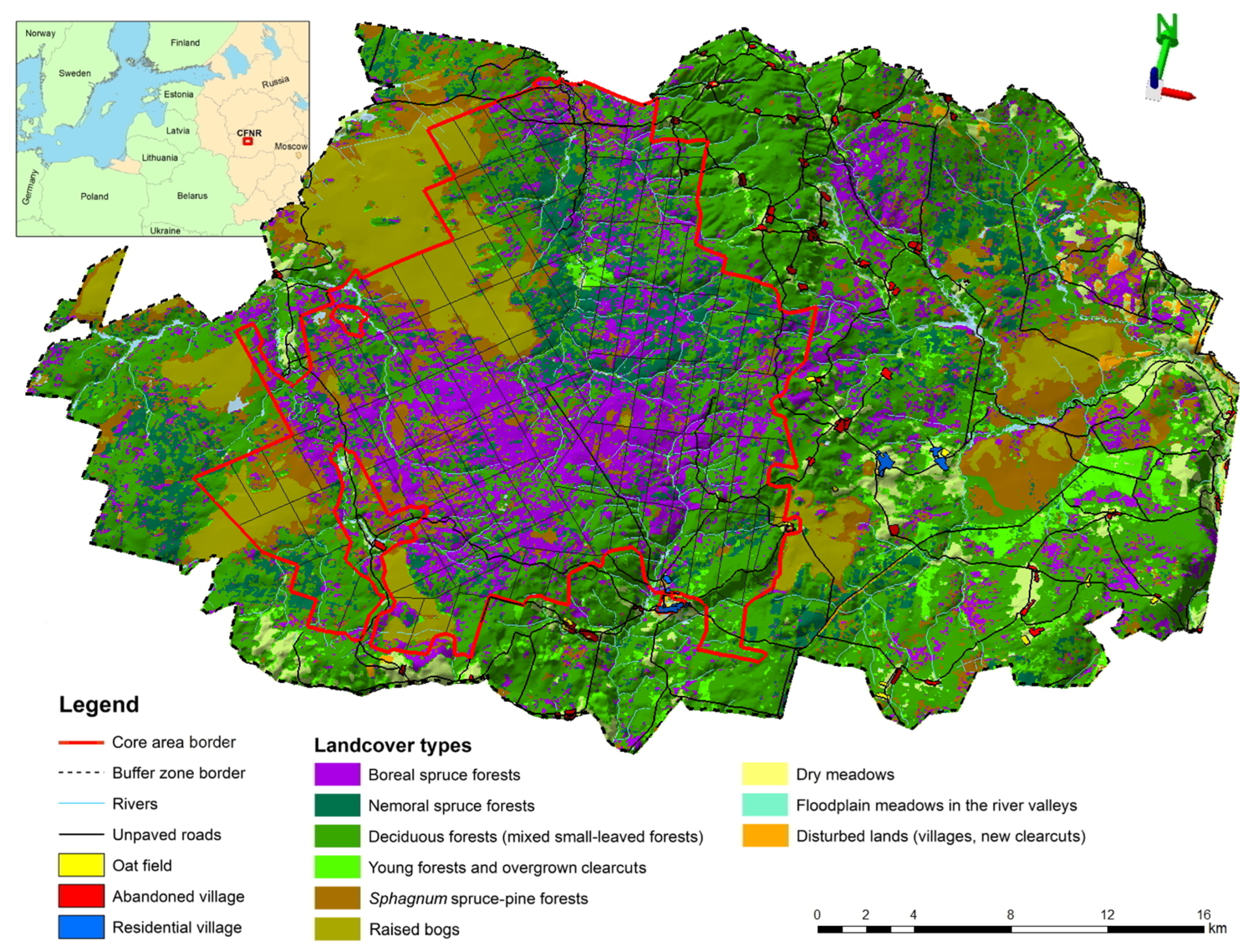
2.1. Study Area

The Central Forest State Nature Biosphere Reserve (hereinafter CFNR) is located in the west of European Russia at the southwestern edge of the Valdai Upland on the Main Caspian–Baltic watershed of the Russian Plain (Tver Region, Russia; 56°25′59″–56°31′01″ N and 32°28′59″–33°01′01″ E; Figure 1). The CFNR territory is characterised by a temperate moderately continental climate with relatively cold winters and warm summers. More than half of the precipitation falls as rain in the summer–autumn period; the remaining amount falls as snow during winter–spring [37]. The mean air temperature of the study area is +4.21 °C (+16 °C in July and −10 °C in January). The mean annual precipitation is 730.9 mm. This territory represents a ridge–hilly elevated plain with absolute elevation of 217–316 m a.s.l. The following geomorphological structures are present here: moraine ridges of Moscow and Valdai age (the latter with well pronounced kames) with elevation of 248–316 m a.s.l., and lake basins with elevation of 217–243 m a.s.l. The CFNR includes a core area (244.15 km2) and a buffer zone (460.61 km2). The terrain of CFNR core area is flat (inclination < 1°) consisting of plains. The drained parts of the moraine ridges are characterised by southern taiga broadleaved–spruce forests and their derivatives. The lake basins and fluvioglacial plains are characterised by boreal spruce forests. The raised bogs are developed on the gentle slopes of moraine ridges and in separate depressions of lake plains. On Sphagnum-dominated raised bogs and their edges, there are plant communities with the participation of Scots pine Pinus sylvestris L. [38]. In general, CFNR core area forests have not been heavily impacted by humans, and they are considered as mostly intact forest areas. At present, windfalls are the only natural drivers of vegetation dynamics.
The buffer zone of the CFNR includes predominantly human-modified landscapes, where active agricultural and forest logging activities occurred until the 1990s. At present, in the CFNR buffer zone, as a result of forest cutting there are many clearcuts of various ages, from young clearcuts without trees to old-growth mixed forests. Nine settlements remain here with a total population of 130–150 people. Only one of them, Zapovedny village, is located in the immediate vicinity of the CFNR core area border. Current meadow plant communities are associated with moraine ridges and represent the cultural landscapes (pastures and hayfields) abandoned before the 1990s and currently overgrown with forest vegetation (Figure 1).
The CFNR forest flora is mainly composed of boreal species widespread in the taiga zone with a dominance of Picea abies L. (hereinafter—spruce) and nemoral species such as Tilia cordata Mill., Corylus avellana L., Ulmus glabra Huds., and U. laevis Pall. Populus tremula L., Betula spp., Alnus incana L., and A. glutinosa L. usually predominate in the disturbed areas after windfalls or forest logging. A special place belongs to Sphagnum-dominated raised bogs and Sphagnum forests with Pinus sylvestris. The CFNR fauna is of European origin, but it includes striking Siberian representatives, the European distributions of which are usually related to boreal landscapes [38]. The common species among large carnivores are brown bear, gray wolf Canis lupus L., and Eurasian lynx Lynx lynx L. Among ungulates, there is a high density of moose Alces alces L. and moderate densities of roe deer Capreolus capreolus L. and wild boar Sus scrofa L.

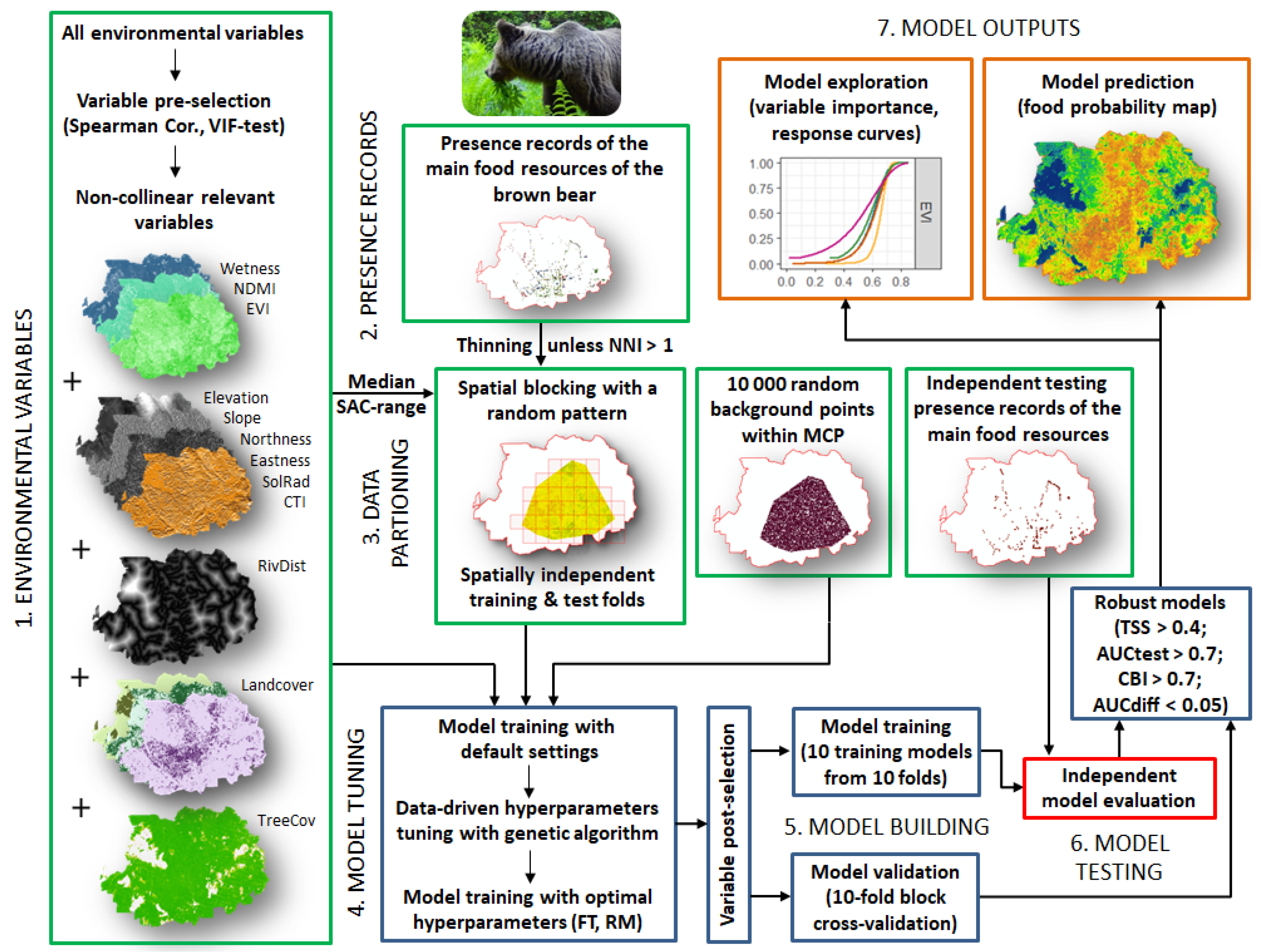
2.2. Food-Probability Models

All key steps for model building are presented according to the general recommendations for SDM studies [4,12]. The model objectives were aimed at studying the relationships between brown bear food resources and their environment (explanation), and mapping their spatial distribution. We describe our models following the Overview, Data, Model, Assessment, Prediction (ODMAP) protocol (ver. 1.0) for SDM [4] with the use of the range model metadata standards (RMMS) dictionary [39]. Here, we provide an overview and the main settings of the distribution models while the remaining ODMAP sections and data processing are detailed in Table S1. The general view of the modelling workflow with the seven main steps is shown in Figure 2. All data processing, analysis, and modelling were done using RStudio 1.1.447 software based on R 4.0.3 [40].
The main food resources of the brown bear have been determined on the basis of a previously conducted diet analysis [41]. We built 14 spatial distribution models for 13 brown bear food resources: Angelica sylvestris L., Aegopodium podagraria L., and Chaerophyllum aromaticum L. individually and all these Apiaceae forbs together, aspen Populus tremula, bilberry Vaccinium myrtillus L., cranberry (Vaccinium microcarpum (Turcz. ex Rupr.) Schmalh. and Vaccinium oxycoccos L., hereinafter Oxycoccus spp.), hazel Corylus avellana, rowan Sorbus aucuparia L., domestic apple Malus domestica Borkh., anthills, social wasps, xylobiont insects, and moose Alces alces. The importance of the main herbaceous plants in the brown bear diet differs within a season (S.S.O., unpublished data), i.e., A. podagraria is important in spring, A. sylvestris in spring and summer, and C. aromaticum in summer. For this reason, we built a general model for all three Apiaceae species and separate models for each of them. We divided all ants into two categories, according to their nest construction: (i) species that build nests with aboveground structure, such as soil nest mounds or anthills from plant remains (anthills); and (ii) species that build nests in dead wood: snags, logs, or stumps (coarse woody debris, according to Frank et al. [42]). The latter category also included the larvae of other xylobionts (mostly beetles), so we combined all insects from coarse woody debris into one category—xylobiont insects. All wasps (yellowjackets) were assigned to the general group of social wasps. On the basis of data from camera traps, brown bears mainly hunted moose in the CFNR during spring and early summer (S.S.O., unpublished data). For this reason, we built a distribution model for moose only for the period of April–June.

2.3. Presence Records of Brown Bear Food Resources

The collection of data on the distribution of brown bear food resources was carried out along hiking routes through the whole study area during March–November of 2008–2020 (Figure A1). We adhered to the general principles for mapping food resources [1,11,36]. In all cases, we recorded the presence of intact (undamaged by brown bears) focus plants and insect nests. Exceptions were the nests of social wasps, dead wood ants, and xylobiont insects, which are difficult to detect if they are not damaged.
Among plants, we recorded only those suitable as brown bear food. For instance, this included all vegetative shoots of herbaceous plants and all dwarf shrubs, regardless of their fruiting. For hazel, this included adult fruiting individuals, and young individuals for aspen and rowan. For each plant species, we recorded its abundance in rectangular “5 m × 5 m” plots using the Braun–Blanquet scale following Shores et al. [36]. In the models, we included as presence records only those locations where the percent cover of a plant was more than 25% (3–5 scores according to the Braun–Blanquet scale). The collection of data on plant distribution was performed using the specially developed form in the ArcGIS QuickCapture (Esri Inc., Redlands, CA, USA) mobile application. We used a specified minimum georeference accuracy of 4.6 m to record the locations of the vegetation plots at their centre. The presence of insects was recorded at each finding of their nests. Moose occurrence was estimated by recording hoof prints, scats, eaten plants, bed sites, and visual observations from April to June, when brown bears intensively prey on adult moose individuals and calves [28,43]. The collection of data on animal distribution was performed using the specially developed form in the ArcGIS Survey123 (Esri Inc., Redlands, CA, USA) mobile application with a given minimum georeference accuracy of 4.6 m (Table S1). To reduce the effects of spatial sampling bias, we thinned all food resource records [44,45,46]. As a measure of clustering, the average nearest neighbour index (NNI) was calculated for both plants and animals using the spatialEco R package [47]. Index values less than 1 exhibit clustering, while values greater than 1 exhibit dispersion or competition [47] (Table A1). The spatial thinning of points was applied with the spThin R package [45]. Thinned points, satisfying a dispersed distribution (NNI > 1), were used as training points for model building.
It is recognised that the filtering (thinning) of species records allows for solving the problem of clustering caused by sampling bias but does not address the issue of spatial autocorrelation (SAC) [48]. Spatial autocorrelation can be observed not only in the model residuals, but also in the input data, i.e., presence records and predictor variables [48,49,50]. Since the calculation of residuals in presence-background models is still controversial, we can only reduce SAC in input datasets. Spatial autocorrelation must be avoided between training and testing data, in order to guarantee independence between them [12], i.e., spatially separated training and testing datasets should be used [48,50]. To account for spatial autocorrelation, we used block cross-validation [49] with a spatial blocking strategy with a random pattern and 100 iterations [50], where the block size was determined from the median of the spatial autocorrelation range among all predictor variables (664 m for plants, 663 m for insects, and 1590 m for mammals) (Figure A2). Ten sets of spatially independent training and test records were performed using the blockCV R package [50].

2.4. Environmental Variables

Climatic, edaphic (soil), and topographical (terrain) variables are most commonly used to model the spatial distribution of plants [11,25,27,33,44,51], while topographical characteristics are more often used for ants [42,52]. In our case, the size of the study area does not allow us to use climatic variables, and edaphic variables are not available at high resolution for the CFNR. We used data from multispectral satellite imagery (vegetation indices, VI), a digital elevation model (DEM), proximity (distance) rasters, landcover types, and forest canopy cover. All of these variables are most often used in modelling food resource distributions at high resolution (30 m) [10,27,35,36].
For the multispectral satellite imagery data, we used nine Landsat 8 OLI-TIRS satellite images [53] (http://www.earthexplorer.usgs.gov; accessed on 10 March 2021) with cloudless coverage of the study area for the period April 2014–October 2020. Whenever possible, two scenes for different years were selected for each month of the vegetative season (Table S1). Before calculating the vegetative indices, a radiometric correction was performed using radiometric coefficients according to the accepted formula [53]. For the first category of predictor variables, we calculated five vegetation indices, including (1) the enhanced vegetation index (EVI) [54], which was developed to correct the vegetation signal through a decoupling of the canopy background signal and a reduction in atmosphere influences. It provides increased sensitivity in areas with dense vegetation and high biomass, while minimising the influence of soil and atmosphere [55]. The EVI is similar to the normalised difference VI (NDVI) [56] and can be used to assess the greenness of vegetation. The other calculated vegetation indices were: (2) the green NDVI (GNDVI), a modification of the NDVI used to assess photosynthetic activity and water consumption by plants [57]; (3) the normalised difference moisture index (NDMI), which measures the moisture content of vegetation [58]; (4) the green chlorophyll VI (GCVI), an estimation of the chlorophyll content in the leaves of various plant species [59]; and (5) the atmospherically resistant VI (ARVI), the first VI that is resistant to atmospheric influences and which also reflects differences in phytomass [60]. For all indices, mean values were calculated on the basis of all Landsat scenes. Additionally, orthogonal vegetation indices were calculated by tasseled cap transformation [61] with corrections for the OLI sensor of the Landsat 8 satellite [62]. Since there were no exposed rocks or large expanses of bare soil in the study area, we did not use brightness. We also did not use greenness, which was highly correlated with EVI. Thus, we used only the third component, wetness, which is a measured value for interactions of soil moisture, water, and other moisture features [62]. It was also calculated as a mean over all Landsat scenes. Calculations of all VI were performed in ArcMap 10.6.1 (Esri Inc., Redlands, CA, USA).
The second category of predictor variables included terrain characteristics calculated from the global DEM (SRTM 1 Arc-Second Global; http://www.earthexplorer.usgs.gov; accessed on 16 November 2018) with a spatial resolution of 30 m, i.e., elevation a.s.l., slope steepness, aspect (northness and eastness), hillshade, and the topographic ruggedness index (TRI) [63]. Before calculating these variables in ArcMap, the DEM layer was projected into UTM 36N according to the recommendations of Sillero and Barbosa [48]. We also calculated the incoming solar radiation (direct insolation) from the DEM. This is also an important variable for building distribution models of animal foraging plants [10,25,27,33,35]. Because soil moisture has been identified as an important predictor for the distribution of brown bear food resources [10,21,25], we calculated the compound topographic index (CTI) [64], also known as the topographic wetness index (TWI) [65], or soil wetness, which is highly correlated with soil moisture. Calculations of solar radiation and CTI were performed in SAGA GIS 7.7.1 [66].
As proximity rasters, distances to rivers were calculated in ArcMap on the basis of 1: 500,000 topographic maps and a panchromatic band of Sentinel-2B satellite images. The landcover types included the following categories: boreal spruce forests, nemoral spruce forests, Sphagnum spruce–pine forests, deciduous mixed small-leaved forests, young forests and overgrown clearcuts, raised bogs, dry meadows, floodplain meadows in river valleys, and disturbed lands (villages and new clearcuts). We defined overgrown clearcuts as secondary forest stands older than 30 years [42]. These data were obtained from our landcover map, which was constructed on the basis of the results of visual classification of Landsat 8 scenes (Figure 1) and performed utilizing the Image Classification tool in ArcMap GIS using the maximum likelihood classification method [67] (Table S1). The resulting map was then compared with ground descriptions and available landcover data from the Global Land Cover service (https://lcviewer.vito.be/; accessed on 5 April 2021). The overall classification accuracy was 88% and kappa was 0.85. For comparison, in similar RSF studies on brown bears, the assessment of the classification accuracy of landscape types ranged from 80 to 88% [1,13,21]. The forest canopy cover was used at a resolution of 30 m (product treecover2010) [68] (data taken from the Global Land Analysis and Discovery—GLAD service; https://glad.umd.edu/; accessed on 26 April 2021).
All environmental variables were transformed to the same geographic extent and WGS84 coordinate system in the UTM 36N projection. A set of 24 preliminary environmental parameters was created at a resolution of 30 m (Table S1). This high resolution did not exceed the permissible error in recording the coordinates (4.6 m) of the presence records [12,48].
All environmental variables were tested for multicollinearity. At the pre-selection step, Spearman’s rank correlation was performed and variables with r > |0.7| were excluded. This included GNDVI, ARVI, and GCVI. Additionally, a variance inflation factor (VIF) test with a threshold value of 10 was performed. The VIF test excluded the forest canopy cover variable for plant food-probability models and EVI for insect models. Because a large number of variables (>15) contribute to model overfitting [69], we also removed TRI and hillshade, as the least ecologically significant ones for the studied species in the CFNR. Floodplain meadow cover (for plant and mammal models) and CTI (for insect models) were deleted during the post-selection step after model fitting because of their low importance values. As a result, a set of 19 environmental variables was obtained, from which subsets of 15 independent environmental variables were compiled for plants, insects, and mammals (Table 1).

2.5. Model Tuning and Calibration (Training)

To build models of spatial distribution, the Maximum Entropy (MaxEnt) algorithm was used, as it is the most optimal for presence-only data [70,71,72,73]. For this we used the Maxent 3.4.1 software [74] freely available on the Internet (https://biodiversityinformatics.amnh.org/open_source/maxent/; accessed on 10 March 2021). Uneven collection of data across a study area inevitably leads to bias and skewed sampling [71], which can distort model realism [75,76]. To correct this error, we created a bias file based on the minimum convex polygon covering all record points [77]. Within this polygon, 10,000 random points were generated, which were indicated to MaxEnt as background samples for comparison [78]. In all cases, a maximum of 1000 iterations and a convergence threshold of 10−5 were used.
Selection of the optimal settings for the model hyperparameters was performed using a genetic algorithm in the SDMtune R package [79]. Combinations of linear, quadratic, product, and hinge feature types were used, as they represent the most appropriate relationships of focal species with environmental variables [78]. The values of the regularization multiplier (RM) were chosen as optimal for data testing and to prevent model overfitting [71,79,80]. The choice of optimal settings was determined by running models in various combinations of the indicated feature types and the RM range from 0 to 8 with a step of 0.5. The final settings for each model are shown in Table 2. To validate such models, k-fold cross-validation was applied using the spatial block method and k = 10 [50]. The best combination of feature types and regularization multiplier was determined using the area under the receiver operating characteristic (ROC) curve (AUC) [81]. After model calibration, a variable reduction procedure was performed (variable post-selection) to remove the least important variables based on the testing true skill statistic (TSS) value [79]. Model tuning, building, and evaluation were performed using the SDMtune [82] and dismo [83] R packages (Table S1).

2.6. Model Evaluation (Testing) and Exploration

For the evaluation of model accuracy, we used different threshold-independent and threshold-dependent metrics [84]. The threshold-independent AUC was used as a measure of model discrimination power. Values of AUC range from 0 to 1, where 1 indicates the model’s perfect ability to differentiate between presence and background points, and 0.5 indicates random-level discrimination [85]. The model with an AUC value > 0.7 suggests that it has good discrimination ability [76,86]. We used AUCtest as the ability of the model to correctly differentiate a random presence point in the test data from a random point of the background [71,75,80]. To assess the overfitting of the model, AUCdiff (the difference between AUCtrain and AUCtest) was calculated. A smaller difference between the values indicates a lower degree of overfitting [84,87]. Because AUC has been somewhat criticised and is not recommended for use as a baseline in assessing the accuracy of presence-only models [87,88], we also used TSS as the main metric. This statistic includes both sensitivity and specificity and can be expressed as sensitivity + specificity −1 [89]. Its values vary from −1 to 1 and follows grades similar to that of the kappa statistic: −1 to 0.40 = poor quality, 0.40 to 0.55 = fair quality, 0.55 to 0.70 = good quality, 0.70 to 0.85 = very good quality, 0.85 to 0.99 = excellent quality [90]. The TSS constitutes a threshold-dependent performance measure, and it was calculated using a TSS-maximization threshold [3,82]. We also utilised the continuous Boyce index (CBI), using the moving window of width W = 0.1 [8,85], to assess the presence probability maps [24]. This index evaluates how strongly the values predicted by the model differ from the randomly expected ones. Its values vary from −1 to 1, where 1 means that the distribution of the predicted values corresponds to the distribution of test values, 0 means the distribution does not differ from the random one, and −1 means that the opposite effect is observed [85]. Because the Boyce index is based on the Spearman rank correlation, we interpreted values > 0.7 (high correlation) as good quality of the model [85]. The CBI was calculated with the help of the ecospat R package [91].
We used multiple lines of independent evidence according to the “gold standard” from Araújo et al. [12]: spatial block cross-validation and held apart fully independent data. Independent test data were taken from the archive of the CFNR. These data were collected by rangers and researchers of the CFNR for the same period of time, independently of the main author. The number of independent test points for each model is shown in Table 2. For each food resource, ten models were tested, built on ten folds of training records according to the partitioning into spatial blocks. In the first case, average TSS, AUCtrain, AUCtest, and AUCdiff values were calculated on the basis of 10-fold block cross-validation. In the second case, the average probability map from the ten models was tested on the independent dataset by calculating the CBI.
To estimate variable importance, we ran a jackknife test removing one variable at a time and calculating the testing TSS to evaluate the final model with the help of the SDMtune R package [79,82]. We also plotted response curves for the most important variables for each food resource.

2.7. Mapping Spatial Distribution

The maps were constructed according to averaged predictions of 10-fold cross-validation models based on the cloglog output format, since we were interested in the presence probabilities of brown bear food resources, with predictions being interpreted as the probability of presence (0 = absence, 1 = presence) [72]. As a threshold for dividing predictions into binary classes (presence/absence of a species) when constructing binary maps, we used the maximum sum of sensitivity plus specificity (maxSSS) threshold value, which is considered to produce the best results for models based on presence-only data [24,92]. For estimating prevalence of each food resource in the CFNR core area and its buffer zone, we calculated area of its presence from a binary map for each territory type and multiplied it by a correction factor (1.32 for the reserve core and 0.68 for the buffer zone). The correction factor was estimated from the proportion of area of each territory type. To build a general map of food resource richness, we combined all binary maps and calculated the sum of the food resource categories for each pixel (Table S1).

3. Results

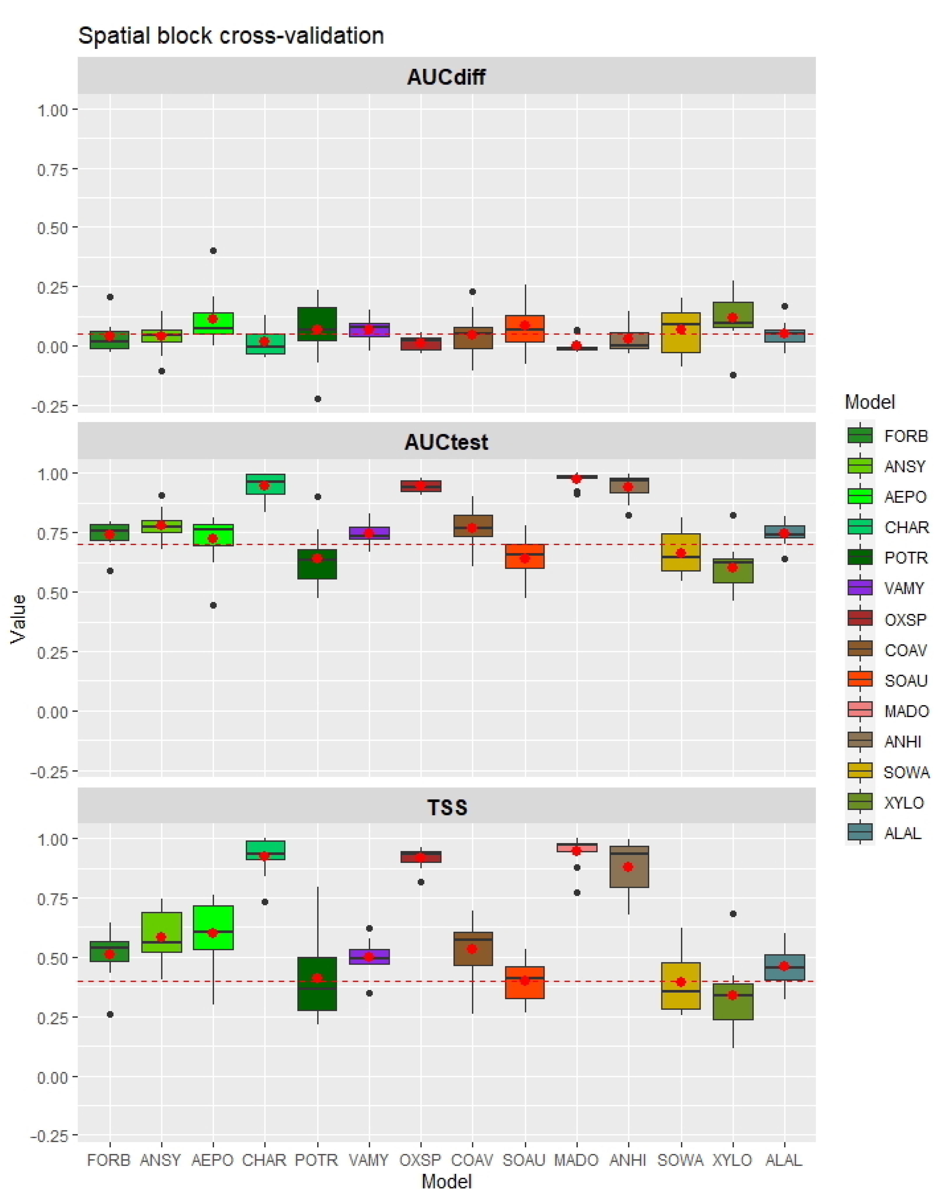
3.1. Evaluation of Food-Probability Models

Among all food-probability models, models for domestic apple (TSS = 0.95), Chaerophyllym aromaticum (TSS = 0.92), cranberry (TSS = 0.92), and anthills (TSS = 0.88) had excellent values of TSS (>0.85). The same models had the highest values of AUCtest and the lowest values of AUCdiff (Table 3; Figure 3). Good estimated values of TSS (0.55–0.70) were found for Aegopodium podagraria (0.60) and Angelica sylvestris (0.59). The AUCtest values of these models were also good (0.72 and 0.78) for Aegopodium podagraria and Angelica sylvestris, respectively. Fair estimates of TSS (0.40–0.55) were obtained for hazel (0.53), Apiaceae spp. (0.51), bilberry (0.50), moose (0.44), aspen (0.41), and rowan (0.40) models. Good AUCtest values were also found for all of these models, except for aspen (0.64) and rowan (0.64). At the same time, maximal CBI values were obtained for moose (0.99), bilberry (0.98), Apiaceae spp. (0.97), hazel (0.97), cranberry (0.95), Aegopodium podagraria (0.93), and Angelica sylvestris (0.92). The following models showed the best CBI curve shapes (in descending order): moose, Apiaceae spp., Angelica sylvestris, bilberry, Aegopodium podagraria, and hazel (Figure 4).
According to TSS values, low quality was noted only for models on xylobiont insects (TSS = 0.34) and social wasps (TSS = 0.39). Taking into account AUCtest values, low quality was found for models on xylobiont insects (0.60), social wasps (0.66), rowan (0.64), and aspen (0.64) (Table 3; Figure 3). At the same time, AUCdiff had maximal values for the xylobiont insects (0.12) and Aegopodium podagraria (0.11) models, which also indicates model overfitting. The value of the continuous Boyce index was lowest for the rowan (CBI = 0.35) and xylobiont insects (CBI = 0.54) models. The most nonlinear shapes of CBI curves were demonstrated by the following models: XYLO (xylobiont insects), ANHI (anthills), SOWA (social wasps), and SOAU (rowan) (Figure 4).
Models for brown bear diet-based RSF were selected on the following basis (in order of importance priority): values of TSS ≥ 0.40 (a quality of higher than fair), AUCtest ≥ 0.70 (good quality), CBI ≥ 0.7 (high correlation and mostly smooth Boyce curves), and AUCdiff ≤ 0.05 (not too overfitted models). Results of the model evaluation are shown in Table 3 and Figure 3. Based on obtained estimates, models on xylobiont insects (XYLO) and social wasps (SOWA) have the lowest predictive ability. In this regard, we cannot include maps of their predictions in the final RSF as reliable predictors of its food resources. POTR (aspen) and SOAU (rowan) models passed the check according to the TSS, but they showed low values of AUCtest, CBI (for rowan), and AUCdiff; thus, they have only been used for building seasonal RSF (spring and autumn, respectively). Models for Aegopodium podagraria (AEPO) and bilberry (VAMY) were overfitted, but they had appropriate values for the other estimates. Therefore, we also retained them in accordance with the priority of importance of estimation criteria.

3.2. Variable Importance

For the Apiaceae spp. model, the most important variables were EVI (TSS = 0.50), NDMI (TSS = 0.33), and DecFor (TSS = 0.31) (Table A2), with which a positive correlation was found (Figure A3). The variable Eastness (TSS = 0.27) was also important; but at the same time, the presence probability of Apiaceae forbs was greatest on southeastern slopes and least on northern slopes (Figure A3). All three Apiaceae species preferred areas with increased values of EVI and NDMI. For the Angelica sylvestris model, the most important variables were the same as for Apiaceae spp., with the addition of Northness (TSS = 0.27), which showed maximal probability of plant presence on southern slopes (Table A2; Figure A3). In addition, the strong positive correlation with the percent cover of mixed small-leaved forests was found only for the A. sylvestris model. For the Aegopodium podagraria model, besides EVI and NDMI, the most important variables were Elevation (TSS = 0.49) and Wetness (TSS = 0.46), while for Chaerophyllum aromaticum, DryMead (TSS = 0.47) was also important. If the probability of A. podagraria presence decreased sharply in high humidity, this decrease was slightly more pronounced for C. aromaticum, which also manifests itself in a less pronounced relationship with an increase in NDMI (Figure A3). At the same time, the probability of A. podagraria presence increased with elevation, while for C. aromaticum the probability of presence increased with increasing percent cover of dry meadows. For the aspen model, the predictors EVI (0.45), Elevation (0.38), NDMI (0.36), and Eastness (0.33) were the most important. With an increase in the values of EVI, Elevation, and NDMI, the probability of aspen presence also increased. In addition, this species also prefers eastern slopes (Figure A3).
For the bilberry model, the variables EVI (TSS = 0.46), NDMI (TSS = 0.35), Wetness (TSS = 0.35), and BorSpr (TSS = 0.33) had the greatest importance (Table A2). Bilberry distribution is associated with low values of EVI and NDMI, increased humidity, and high percent cover of boreal spruce forests (Figure A4). For cranberry, the most important variables were RaisBog (TSS = 0.88), Wetness (TSS = 0.80), Elevation (TSS = 0.69), and NDMI (TSS = 0.51). The probability of cranberry presence was directly related to the percent cover of raised bogs. At the same time, the probability of cranberry presence decreased sharply with an increase in humidity (Figure A4).
For the hazel model, the most important variables were EVI (TSS = 0.48), DecFor (TSS = 0.47), Wetness (TSS = 0.43), and NDMI (TSS = 0.36), with which the model was correlated positively (Table A2; Figure A4). Only for Elevation did we find a sharp decrease with a consequent increase in presence probability. For the rowan model, the variables Elevation (TSS = 0.38), NDMI (TSS = 0.31), BorSpr (TSS = 0.31), and Wetness (TSS = 0.30) were the most important. Rowan preferred areas of elevated terrain, but this species was also able to inhabit wet locations. In addition, the model revealed the wide distribution of rowan in the study area, including the understory of boreal spruce forests. For domestic apple, the highest TSS values were found for the variables Wetness (TSS = 0.89), EVI (TSS = 0.88), DryMead (TSS = 0.79), and Eastness (TSS = 0.53). Domestic apple preferred dry meadows with a small amount of soil moisture, as its presence probability decreased with an increase in soil moisture and was associated with western and eastern slopes (Figure A4).
For the anthills model, the variables DryMead (TSS = 0.83), Wetness (TSS = 0.76), EVI (TSS = 0.75), TreeCov (TSS = 0.67), and DecFor (TSS = 0.41) were the most important (Table A2). Response curves indicated the preference of ants for dry meadows with rich herbaceous vegetation, dry soils, and moderate (up to 60%) tree canopy cover (Figure A5). According to the model, ants can inhabit sparse, well-illuminated forests and forest edges. For moose, the most important variables were EVI (TSS = 0.30), DecFor (TSS = 0.23), Elevation (TSS = 0.21), Wetness (TSS = 0.20), RivDist (TSS = 0.19), and TreeCov (TSS = 0.18). In spring and early summer, moose preferred river floodplains with rich herbaceous vegetation and sparse mixed forests (Figure A5).

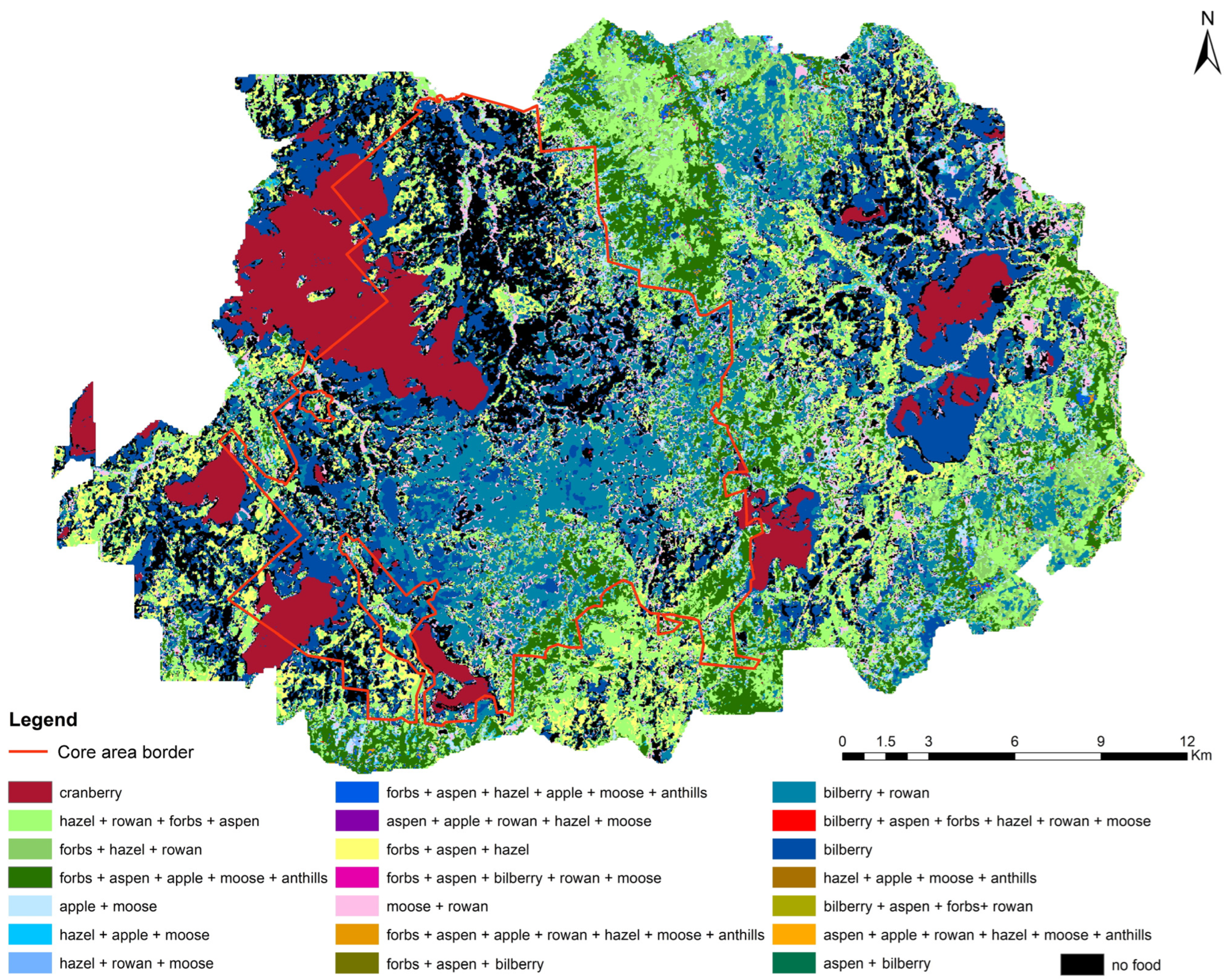
3.3. Food-Probability Maps

Predicted food presence probability maps were generated for all reliable models (Figure 5). According to the maps, we can assume that the vast majority of brown bear food resources were prevalent in the CFNR buffer zone, while only bilberry was much more widespread in the CFNR core area (Figure 6). Cranberry and rowan had more or less equal prevalence in both territories. By combining the predicted maps of food resource distribution, we obtained a general map reflecting the richness of brown bear food resources in the study area (Figure 7 and Figure A6). Again, food richness was more relevant in the CFNR buffer zone than within its core area. Actually, the CFNR core area was characterised by twice as many areas without food resources (21%) as compared to the CFNR buffer zone (11.5%). In addition, in the CFNR core area there was a higher proportion of areas with one or two types of food resources (Table 4), while the CFNR buffer zone had considerably more areas with three to six different types of food resources. Finally, unique areas where all seven food resource types occur together were found only in the CFNR buffer zone.

4. Discussion

The abundance and distribution of main food resources determine seasonal and annual variations in their consumption, together with the spatial distribution, behaviour, demography [27,34,93], and habitat selection of the brown bear [10,26,94]. At the same time, food resource attractiveness is determined by not only its spatial distribution affecting the time required for its search and consumption, but also its energy value and local abundance [95]. As a result, spatial variations of food resources have a great impact on habitat suitability for the brown bear [96].
The use of direct food resource variables in brown bear habitat suitability modelling is largely based on a thorough study of its trophic ecology, including knowledge of diet, seasonal dynamics of food consumption, food resource energy values, and the characteristics of resource usage [10]. Such studies are necessary for a deeper understanding of the relationship between a species and the habitats producing its main food resources, and the peculiarities of the distribution of individuals across its territory [97,98,99].
According to the estimates obtained, most of our food-probability models predict the distribution of food resources over the study area quite well. The values of TSS ranged from 0.34 to 0.95. For example, forage plant distribution models for the brown bear in Alberta (Canada) were of inferior quality; their kappa estimates (which can be regarded as analogous to TSS) ranged from 0.09 to 0.48 [35]. At the same time, Penteriani et al. [33] obtained TSS estimates for brown bear food resources in the Cantabrian Mountains ranging from 0.52 to 0.75.
Spatial autocorrelation reduction and the thinning of presence records deserve special attention. The problem of SAC influence on the results of modelling using MaxEnt is still controversial [100,101,102,103]. Until now, the easiest way to solve this has been to avoid the spatial dependence of the training and test datasets [12,48,50]. By avoiding the problem of spatial sampling bias by rarefying the points, we considerably reduce the information available for training the model. Some of the studied species (cranberry, Chaerophyllum aromaticum, domestic apple, ant species with soil nest mounds) inhabit limited areas under specific conditions. For such plants and animals, the thinning of presence records reduced the realism of the obtained maps and was reflected in the highly nonlinear CBI curves.
The SDMs of herbaceous plants turned out to be quite reliable both for the whole group (TSS = 0.51) and for individual species in particular (TSS = 0.59–0.92). For example, model quality check for Hedysarum alpinum L. in Alberta (Canada) had a kappa value of 0.48 [35]. Models for Angelica sylvestris and Aegopodium podagraria had the lowest values of quality assessment among herbaceous plants. This is caused by the wide distribution of these species in the study area and their ability to inhabit both meadows and forests, including forest edges [104,105].
In general, the distribution of Apiaceae forbs was associated with areas having rich phytomass and moist conditions on southeastern slopes. The distribution of Angelica sylvestris was associated with the percent cover of mixed forests and southern slopes. The main habitats of this species were sparse forests (small forest edges and glades, open gaps in forests, forest roads, and narrow clearings) and the periphery of overgrown meadows, which are ecotone habitats. This is confirmed by its ability to renew itself with the help of renewal buds in case of damage [106], particularly that of being eaten by the brown bear, and its wide environmental valence in the study area [107].
The distribution of Aegopodium podagraria was similar to that of Angelica sylvestris, but it was also influenced by elevation and soil moisture. In contrast to A. sylvestris, based on our model, A. podagraria was to a greater extent confined to wet (but not waterlogged) soils, and to elevated terrain. This is confirmed by data on the ecological preferences of the species when A. podagraria is widespread throughout a study area, as its habitats are associated with moist tallgrass broadleaved–spruce and small-leaved forests [105]. According to our observations, it often preferred former farmlands and backyards in abandoned villages and their surroundings. The adaptability of A. podagraria to a wider range of habitats can be determined by its ability to adapt at the physiological level to various environmental conditions [108], although this species grows better in higher illumination conditions [107].
The distribution of Chaerophyllum aromaticum was associated to a greater extent with dry meadows than with forests. Unlike Aegopodium podagraria, C. aromaticum more strongly avoided waterlogged soils and was more associated with EVI, preferring areas in dry meadows rich in phytomass. This species was especially widespread within abandoned settlements, forming large thickets in former vegetable gardens with fertile soils. This is partly a consequence of the burrowing activity of wild boars Sus scrofa, which dig up the soil in dry meadows, feeding on the plant rhizomes. Thus, these animals create favourable conditions for C. aromaticum seeds, which, as early as the following year, can germinate at sites dug by wild boars. For this reason, C. aromaticum distribution was so strongly influenced by the percent cover of dry meadows. In the Smolensk Region, a short distance south of the study area, a plant community with a predominance of this species was recently described, namely the association Scirpo sylvatici–Alnetum incanae variant C. aromaticum [109]. It was noted that this plant community was formed in disturbed habitats in the vicinity of settlements on the richest and moistest loamy soils [109].
The aspen range covers all of Eurasia, from Iceland to the Russian Far East and from northern Scandinavia to the Mediterranean coast of Africa [110]. In forests of the taiga zone, aspen is a pioneer species of post-fire successions, and it is associated with many species of animals, bryophytes, and lichens in boreal forests [111]. Our model for aspen was not very reliable, as its AUCtest did not reach the lower threshold value of reliability. Most likely, this was caused by the wide distribution of aspen in the study area and by limiting the sampling to only young trees suitable for brown bear consumption. Our model was able to reveal that young individuals of this tree species preferred small-leaved mixed forests, mainly on elevated areas and eastern slopes, with high EVI and NDMI values. This is generally consistent with the environmental requirements of aspen [107,110,111,112].
Bilberry is a widely distributed species in many European regions associated with boreal forests [44,113,114]. In the study area, it is found in boreal spruce forests, Sphagnum spruce forests, and pine forests in areas surrounding raised bogs [105]. In this regard, there was a tendency towards wet areas with low values of EVI and NDMI, which was convincingly shown by our model, together with a close relationship with boreal spruce forests and Sphagnum spruce–pine forests. Bilberry distribution was also influenced by the sum of temperatures; however, it manifests itself mainly indirectly due to the predictors of elevation and forest type, as demonstrated in other studies, e.g., [114]. In our case, bilberry avoided deciduous forests, while it preferred boreal spruce forests and Sphagnum spruce–pine forests. In the boreal forests of Finland, bilberry abundance in pine forests was 1.13 times higher than that in spruce forests, due to different illumination conditions [114]. Our field observations also confirm this. In the study area, however, boreal spruce forests are distributed wider than Sphagnum pine forests. Therefore, the value of Sphagnum spruce–pine forests in our model was slightly lower (TSS = 0.22) than that of spruce forests (TSS = 0.33). Estimates of the quality of models for bilberry turned out to be quite high (AUCtest = 0.75 and TSS = 0.50) and generally in agreement with those in other studies. For example, Penteriani and coauthors [33] found the following estimates for models of bilberry in the Cantabrian Mountains: AUC = 0.94 and TSS = 0.52. Nijland et al. [35] observed lower estimates for models of Vaccinium cespitosum Michx. (kappa = 0.32) and V. vitis-idaea L. (kappa = 0.38) in Alberta, Canada. Bilberry was the only food source whose distribution was associated more with the natural landscapes in the reserve core area than the human-modified buffer zone, which was also confirmed by our previous work [41]. This is explained by the active logging of boreal forests everywhere in the surrounding area in both the past and the present, and only because of the protected status of the reserve core area do the large expanses of intact boreal forests still persist to the present time.
Vaccinium microcarpum and V. oxycoccos are distributed in raised bogs. Both species inhabit raised bogs of the CFNR core area and buffer zone and Sphagnum pine forests. Thus, their distribution was associated with the percent cover of raised bogs and with depressions in the terrain. At the same time, the model revealed the avoidance of raised bog areas oversaturated with water, which is also consistent with environmental preferences of both species [115].
Hazel is the typical inhabitant in the understory of broadleaved and mixed forests in Europe [116]. According to the COAV model, in the study area, hazel was confined to mixed forests, where it grows in the understory. Such areas have higher EVI values. We noted that hazel was confined to elevated areas, but at the same time, this species can also exist under certain soil moisture levels. Estimates of model quality for hazel were at the good level (AUCtest = 0.77 and TSS = 0.53). However, our estimates were lower than those in models for species with a similar food value, such as Fagus sylvatica L. (AUC = 0.97 and TSS = 0.75) and Castanea sativa Mill. (AUC = 0.89 and TSS = 0.54), for bears in the Cantabrian Mountains [33].
According to the SOAU model, the distribution of rowan was mainly determined by the presence of mixed and deciduous forests in areas of elevated terrain, which is consistent with the results of models in other studies, e.g., [51]. However, in our case, the models revealed that rowan (in a depressed state) can also grow in the understory of coniferous forests, including boreal ones, where this species successfully lives in moist soils. Although surviving in such conditions, rowan productivity in this area is very low, as there are practically no fruits. The model for this species has a borderline TSS value (0.40) and a low AUCtest value (0.64), which is also associated with its wide distribution in the study area. At the same time, Mellert with coauthors [51] reported an AUCtest value of 0.68 for rowan, which is slightly greater than our estimate.
The distribution of domestic apple was related to past human activity in the study area. The CFNR buffer zone was densely populated 40 years ago. There were many villages and agricultural activities were carried out. In all the villages, people cultivated orchard apples, which had a great taste. Despite the fact that most of the villages were abandoned back in the 1980s, the remaining apple orchards still continue to actively produce fruit. Many trees have retained the good taste of their apples, which serve as a favourite food for bears in the study area.
Almost all the villages were located along moraine–kame ridges, which are related to the Valdai glaciation, and found primarily in the CFNR buffer zone. The study area has generally poor soils for agriculture. The cultivation of various crop plants was possible only on partially drained soils in elevated areas of moraine–kame ridges. In such places, villages existed for a long time. Around these villages, the forest was cut down, and arable lands, pastures, and hayfields appeared. Today, in these places there are dry meadows, which are actively overgrown with forest vegetation [38]. This was confirmed by our model, which indicated that domestic apple distribution was associated primarily with dry soils in dry meadows with rich herbaceous vegetation (and, as a consequence, high EVI values) on western and eastern (but not northern) slopes.
Our anthills model was very similar and showed that soil nest mounds were associated primarily with dry meadows with rich herbaceous vegetation (high EVI values), dry soils, and not high tree canopy cover. These landscapes were also associated with abandoned pastures and hayfields in the CFNR buffer zone. Field observations demonstrated that Lasius niger L. and Formica fusca L. often inhabit such places, as well as overgrown forest glades and forest roadsides, where Formica pratensis Retz., Formica exsecta Nyl., and Myrmica rubra L. live, and even along the edges of raised bogs (L. niger, M. rubra). It is known that dry soils and high illumination are among the most important factors for many ant species from this [52,117] and other groups [118]. This has been confirmed by other studies. For example, in Transylvania (Romania), nests of Lasius flavus F., L. niger, and Tetramorium caespitum L. were distributed in wood-pastures, i.e., meadows, with partial shrub and tree cover [117], as were anthills in the Slovakian Pol’ana Mountains [119]. However, in the study area, soil ants also often inhabit roadsides, small forest glades, and forest edges, which was also confirmed by our model.
The model for moose had a relatively low TSS value (0.44), which was associated with the wide distribution of this species in the study area. It is a common species inhabiting almost all possible habitats in both the core area and buffer zone of the CFNR. Having no telemetry data, it is very difficult to reliably predict moose distribution even in a particular time period. Nevertheless, our model ALAL was able to reveal moose preferences in spring and early summer for river floodplains with rich phytomass and sparse mixed forests. After the winter and with the beginning of vegetation growth, moose actively consume young vegetation, including that found in floodplains (e.g., Equisetum spp., Filipendula ulmaria L., Sonchus spp.). In central Norway, moose selected good foraging habitats in spring, such as young forest stands and cultivated land, and older forests as shelter habitats. At the same time, reproducing females avoided open, food-rich areas in the first months after their calves were born, whereas males and females without young selected these areas in spring and summer [120].
In general, we found that the territory of the CFNR buffer zone contains a higher variety of brown bear food resources than the CFNR core area. According to the built models, the presence of up to seven food resources was predicted in the CFNR buffer zone. All main food resources apart from bilberry were more prevalent in the buffer zone. This is explained by a set of different factors. Terrain origin associated with the Valdai glaciation determined the nature of human land use and human settlement on elevated areas of moraine–kame ridges. Human agricultural and logging activities in these places modified the landscape and created a mosaic of heterogeneous landscapes (dry meadows overgrown with forest vegetation, secondary mixed forests, forest glades, and clearcuts) [38], which have high productivity for most food resources favoured by brown bears to the present time. Moreover, the distribution of many food resources, such as apples, hazelnuts, anthills, and many herbaceous plants, were associated mainly with these types of landscapes, which was demonstrated by our models.
On the basis of these results, the human-modified CFNR buffer zone seems to be more suitable for brown bears from a nutritional point of view in comparison to the natural landscapes of the CFNR core area. Strictly protected since 1931, spruce forests of the CFNR core area became overmature and have low nutritional value for brown bears. Only bilberry had greater prevalence in the core area, which was also confirmed by our previous work [41].

5. Conclusions

We believe that when building habitat suitability models for the brown bear it is necessary to use proximal resource variables instead of their environmental surrogates. With the help of additional field studies, it is possible to build food-probability models for further RSF with direct resources, or as we call them real RSFs. This can lead us not to assumptions, but to direct logical connections between a species and its resources and habitats. Combined maps of food resource distribution allowed us to conclude that the territory of the human-modified CFNR buffer zone contains a higher variety of food resources than the strictly protected CFNR core area, where there is a concentration of closed, intact spruce forests of boreal and nemoral structure. More research is thus needed to understand the real impact of protected areas on the conservation and management of brown bear populations (and, more generally, on large carnivore populations) compared to larger, less protected landscapes in human-modified regions. Actually, the typical large displacements of brown bears [121] increase the interactions that this species may have with areas characterised by diverse protection rules, a factor that needs to be addressed in conservation and management plans.

Supplementary Materials

The following supporting information can be downloaded at: www.mdpi.com/article/10.3390/f13081247/s1, Table S1: ODMAP Protocol (ver. 1.0) for food-probability models for the brown bear in the Central Forest State Nature Biosphere Reserve (West-European Russia) (Details on Data, Model, Assessment, and Prediction). References [122,123,124,125,126,127,128] are cited in the supplementary materials file available at the link above.

Author Contributions

S.S.O. designed the study, collected field data for model building, performed the modelling, wrote the protocol, and developed the research idea through discussion with M.d.M.D. and V.P.; A.S.Z. collected field data for independent model evaluation; S.S.O. and A.A.K. prepared the first draft of the manuscript; A.A.K. performed the botanical component of the work; E.B.F. identified all ant specimens; A.V.A. identified all wasp specimens; E.B.F. and A.V.A. performed the entomological component of the work; V.P. supervised all work; V.P., M.d.M.D., A.S.Z., E.B.F. and A.V.A. edited, significantly improved, and finalised the manuscript; A.A.K. and V.P. supported publication of this work. All authors have read and agreed to the published version of the manuscript.

Funding

The study of A.K. was performed within the framework of the state assignment FEWZ-2020-0009 from Ministry of Education and Science of the Russian Federation. During this work, V.P. was supported by the I+D+i Project PID2020-114181GB-I00 financed by the Spanish Ministry of Science and Innovation, the Agencia Estatal de Investigación (AEI), and the Fondo Europeo de Desarrollo Regional (FEDER, EU).

Institutional Review Board Statement

Not applicable.

Informed Consent Statement

Not applicable.

Data Availability Statement

All data descriptions are presented in the ODMAP protocol. The data presented in this study are available on request from the corresponding author.

Acknowledgments

Authors appreciate the rangers and researchers of the CFNR for providing field data for the independent model evaluation.

Conflicts of Interest

The authors declare no conflict of interest. The funders had no role in the design of the study; in the collection, analyses, or interpretation of data; in the writing of the manuscript; or in the decision to publish the results.

Appendix A

Table A1. Check for spatial clustering with the average nearest neighbour index (NNI), its z-score, and p-level for 14 brown bear food-probability models in the Central Forest State Nature Reserve (West-European Russia) in 2008–2020.
Model NameRarefy Distance (m)NNIz-Scorep-Value
FORB5001.091.540.12
ANSY4501.101.570.12
AEPO2201.060.680.50
CHAR2701.272.180.03
POTR301.172.270.02
VAMY3701.162.790.01
OXSP6500.88–1.090.28
COAV3501.071.160.25
SOAU4401.111.720.09
MADO7201.010.120.91
ANHI5601.040.530.60
SOWA4901.091.300.19
XYLO1401.071.140.25
ALAL4401.102.740.01
Note: FORB—Apiaceae spp., ANSY—Angelica sylvestris, CHAR—Chaerophyllym aromaticum, AEPO—Aegopodium podagraria, POTR—Populus tremula, VAMY—Vaccinium myrtillus, OXSP—Oxycoccus spp., COAV—Corylus avellana, SOAU—Sorbus aucuparia, MADO—Malus domestica, ANHI—anthills, SOWA—social wasps, XYLO—xylobiont insects, ALAL—Alces alces.
Table A2. Jackknife test for variable importance after removing one variable at a time for 14 food-probability models for the brown bear in the Central Forest State Nature Reserve (West-European Russia) in 2008–2020 using the metric TSS with running the test for one single variable. The first four most important variables are marked in bold. Variable abbreviations are the same as in Table 1.
VariableFORBANSYAEPOCHARPOTRVAMYOXSPCOAVSOAUMADOANHIALAL
EVI0.500.560.600.910.450.460.230.480.160.880.750.30
NDMI0.330.440.390.500.360.350.510.360.310.020.15
Wetness0.020.210.460.760.280.350.800.430.300.890.760.20
Elevation0.080.170.490.420.380.300.690.390.380.000.020.21
Slope0.37
Northness0.220.270.280.010.250.080.020.150.190.480.240.06
Eastness0.270.260.260.350.330.170.000.230.190.530.210.16
CTI0.110.120.300.290.020.250.160.280.260.00
SolRad0.220.240.290.000.010.030.020.230.020.12
RivDist0.19
BorSpr0.220.220.160.320.150.330.390.280.310.300.300.14
NemSpr0.140.150.110.140.140.080.220.190.110.170.180.12
SphFor0.140.140.110.160.130.220.000.080.100.130.150.09
DecFor0.310.300.360.000.240.310.500.470.000.480.410.23
YoungFor0.130.160.120.220.100.050.000.050.020.000.310.10
RaisBog0.050.050.050.050.060.040.880.010.030.030.050.05
DryMead0.090.110.140.470.000.050.000.020.050.790.830.07
FloodMead0.07
TreeCov0.670.18
Figure A1. Sampling routes on the distribution of brown bear food resources in the territory of the Central Forest State Nature Reserve core area and buffer zone during March–November of 2008–2020.
Forests 13 01247 g0a1
Figure A2. Output graphs from the R package blockCV showing spatial autocorrelation ranges for input predictor variables before fitting 14 food-probability models for the brown bear in the Central Forest State Nature Reserve (West-European Russia) in 2008–2020. Variable subsets for (A) plant models, (B) insect models, and (C) mammal models are shown. For each variable subset, selected block size based on median spatial autocorrelation range across all input predictors is shown.
Forests 13 01247 g0a2
Figure A3. Response curves for the four most important variables of the brown bear vegetative food-probability models (forbs and tree leaves) in the Central Forest State Nature Reserve (West-European Russia) in 2008–2020. Designations: FORB—Apiaceae species, ANSY—Angelica sylvestris, CHAR—Chaerophyllym aromaticum, AEPO—Aegopodium podagraria, and POTR—Populus tremula. The curves show the mean response of the ten cross-validation MaxEnt runs and the mean ± one standard deviation. EVI—enhanced vegetation index; NDMI—normalised difference moisture index; Wetness—tasseled cap wetness; Elevation—elevation (m a.s.l.); Northness—northness (aspect) from the digital elevation model; Eastness—eastness (aspect) from the digital elevation model; SolRad—solar radiation; BorSpr—proportion of boreal spruce forests (%); DecFor—proportion of deciduous forests (mixed small-leaved forests) (%); DryMead—proportion of dry meadows (%). Units of the variables are shown in Table 1 of the main text.
Forests 13 01247 g0a3
Figure A4. Response curves for the four most important variables of the brown bear fruit food-probability models (soft and hard mast) in the Central Forest State Nature Reserve and its buffer zone (European Russia) in 2008–2020. Designations: VAMY—Vaccinium myrtillus, OXSP—Oxycoccus spp., COAV—Corylus avellana, SOAU—Sorbus aucuparia, and MADO—Malus domestica. The curves show the mean response of the ten cross-validation MaxEnt runs and the mean ± one standard deviation. EVI—enhanced vegetation index; NDMI—normalised difference moisture index; Wetness—tasseled cap wetness; Elevation—elevation (m a.s.l.); Eastness—eastness (aspect) from the digital elevation model; CTI—compound topographic index; BorSpr—proportion of boreal spruce forests (%); SphFor—proportion of Sphagnum spruce–pine forests (%); DecFor—proportion of deciduous forests (mixed small-leaved forests) (%); RaisBog—proportion of raised bogs (%); DryMead—proportion of dry meadows (%). Units of the variables are shown in Table 1 of the main text.
Forests 13 01247 g0a4
Figure A5. Response curves for the five (insects) and six (mammals) most important variables of the brown bear animal food-probability models in the Central Forest State Nature Reserve and its buffer zone (European Russia) in 2008–2020. Designations: ANHI—anthills, ALAL—Alces alces. The curves show the mean response of the ten cross-validation MaxEnt runs and the mean ± one standard deviation. EVI—enhanced vegetation index; Wetness—tasseled cap wetness; Elevation—elevation (m a.s.l.); RivDist—distance to rivers; DecFor—proportion of deciduous forests (mixed small-leaved forests) (%); YoungFor—proportion of young forests and overgrown clearings (%); DryMead—proportion of dry meadows (%); TreeCov—forest canopy cover. Units of the variables are shown in Table 1 of the main text.
Forests 13 01247 g0a5
Figure A6. The global map of brown bear food resource richness in the Central Forest State Nature Reserve (West-European Russia) in 2008–2020 showing individual food objects. The colours indicate different combination of food resources (one to seven) per pixel among the following items: Apiaceae forbs, aspen, bilberry, cranberry, hazel, rowan, domestic apple, anthills, and moose. The CFNR core area is inside the red line polygon; the CFNR buffer zone is outside the red line polygon.
Forests 13 01247 g0a6

References

  1. Nielsen, S.E.; Boyce, M.S.; Stenhouse, G.B.; Munro, R.H.M. Development and testing of phenologically driven grizzly bear habitat models. Écoscience 2003, 10, 1–10. [Google Scholar] [CrossRef]
  2. Milakovic, B.; Parker, K.L.; Gustine, D.D.; Lay, R.J.; Walker, A.B.D.; Gillingham, M.P. Seasonal habitat use and selection by grizzly bears in Northern British Columbia. J. Wildl. Manag. 2012, 76, 170–180. [Google Scholar] [CrossRef]
  3. Guisan, A.; Thuiller, W.; Zimmermann, N.E. Habitat Suitability and Distribution Models; Cambridge University Press: Cambridge, UK, 2017; 462p. [Google Scholar]
  4. Zurell, D.; Franklin, J.; König, C.; Bouchet, P.J.; Dormann, C.F.; Elith, J.; Fandos, G.; Feng, X.; Guillera-Arroita, G.; Guisan, A.; et al. A standard protocol for reporting species distribution models. Ecography 2020, 43, 1261–1277. [Google Scholar] [CrossRef]
  5. Boyce, M.S.; McDonald, L.L. Relating populations to habitats using resource selection functions. Trends Ecol. Evol. 1999, 14, 268–272. [Google Scholar] [CrossRef]
  6. Franklin, J. Mapping Species Distributions: Spatial Inference and Prediction; Cambridge University Press: Cambridge, UK, 2010; 320p. [Google Scholar]
  7. Manly, B.F.J.; McDonald, L.L.; Thomas, D.L.; McDonald, T.L.; Erickson, W.P. Resource Selection by Animals. Statistical Design and Analysis for Field Studies, 2nd ed.; Kluwer Academic Publishers: Dordrecht, The Netherlands, 2002; 221p. [Google Scholar]
  8. Boyce, M.S.; Vernier, P.R.; Nielsen, S.E.; Schmiegelow, F.K.A. Evaluating resource selection functions. Ecol. Model. 2002, 157, 281–300. [Google Scholar] [CrossRef]
  9. Austin, M.P. Spatial prediction of species distribution: An interface between ecological theory and statistical modelling. Ecol. Model. 2002, 157, 101–118. [Google Scholar] [CrossRef]
  10. Nielsen, S.E.; McDermid, G.; Stenhouse, G.B.; Boyce, M.S. Dynamic wildlife habitat models: Seasonal foods and mortality risk predict occupancy-abundance and habitat selection in grizzly bears. Biol. Conserv. 2010, 143, 1623–1634. [Google Scholar] [CrossRef]
  11. Nielsen, S.E.; Larsen, T.A.; Stenhouse, G.B.; Coogan, S.C.P. Complementary food resources of carnivory and frugivory affect local abundance of an omnivorous carnivore. Oikos 2016, 126, 369–380. [Google Scholar] [CrossRef]
  12. Araújo, M.; Anderson, R.; Barbosa, A.M.; Beale, C.; Dormann, C.; Early, R.; Garcia, R.; Guisan, A.; Maiorano, L.; Naimi, B.; et al. Standards for distribution models in biodiversity assessments. Sci. Adv. 2019, 5, eaat4858. [Google Scholar] [CrossRef]
  13. Nielsen, S.E.; Boyce, M.S.; Stenhouse, G.B.; Munro, R.H.M. Modeling grizzly bear habitats in the Yellowhead ecosystem of Alberta: Taking autocorrelation seriously. Ursus 2002, 13, 45–56. [Google Scholar]
  14. Lyons, A.L.; Gaines, W.L.; Servheen, C. Black bear resource selection in the northeast Cascades, Washington. Biol. Conserv. 2003, 113, 55–62. [Google Scholar] [CrossRef]
  15. Hiller, T.L.; Belant, J.L.; Beringer, J.; Tyre, A.J. Resource selection by recolonizing american black bears in a fragmented forest landscape. Ursus 2015, 26, 116–128. [Google Scholar] [CrossRef]
  16. Lone, K.; Merkel, B.; Lydersen, C.; Kovacs, K.; Aars, J. Sea ice resource selection models for polar bears in the Barents Sea subpopulation. Ecography 2017, 41, 567–578. [Google Scholar] [CrossRef]
  17. Bai, W.; Huang, Q.; Zhang, J.; Stabach, J.; Huang, J.; Yang, H.; Songer, M.; Connor, T.; Liu, J.; Zhou, S.; et al. Microhabitat selection by giant pandas. Biol. Conserv. 2020, 247, 108615. [Google Scholar] [CrossRef]
  18. Ciarniello, L.M.; Boyce, M.S.; Beyer, H. Resource Selection Function for the Plateau Landscape of the Parsnip Grizzly Bear Project (An Update for 2003); Technical Report; British Columbia Ministry of Forests: Vancouver, BC, Canada, 2003; p. 18.
  19. Ciarniello, L.M.; Boyce, M.S.; Heard, D.C.; Seip, D.R. Components of grizzly bear habitat selection: Density; habitats; roads; and mortality risks. J. Wildl. Manag. 2007, 71, 1446–1457. [Google Scholar] [CrossRef]
  20. Wiegand, T.; Naves, J.; Garbulsky, M.F.; Fernandez, N. Animal habitat quality and ecosystem functioning: Exploring seasonal patterns using NDVI. Ecol. Monogr. 2008, 78, 87–103. [Google Scholar] [CrossRef]
  21. Chetkiewicz, C.L.B.; Boyce, M.S. Use of resource selection functions to identify conservation corridors. J. Appl. Ecol. 2009, 46, 1036–1047. [Google Scholar] [CrossRef]
  22. Graves, T.A.; Kendall, K.C.; Royle, J.A.; Stetz, J.B.; Macleod, A.C. Linking landscape characteristics to local grizzly bear abundance using multiple detection methods in a hierarchical model. Anim. Conserv. 2011, 14, 652–664. [Google Scholar] [CrossRef]
  23. Peters, W.; Hebblewhite, M.; Cavedon, M.; Pedrotti, L.; Mustoni, A.; Zibordi, F.; Cagnacci, F. Resource selection and connectivity reveal conservation challenges for reintroduced brown bears in the Italian Alps. Biol. Conserv. 2015, 186, 123–133. [Google Scholar] [CrossRef]
  24. Recio, M.R.; Knauer, F.; Molinari-Jobin, A.; Huber, D.; Filacorda, S.; Jerina, K. Context-dependent behaviour and connectivity of recolonizing brown bear populations identify transboundary conservation challenges in Central Europe. Anim. Conserv. 2020, 24, 73–83. [Google Scholar] [CrossRef]
  25. Roberts, D.R.; Nielsen, S.E.; Stenhouse, G.B. Idiosyncratic responses of grizzly bear habitat to climate change based on projected changes in their food resources. Ecol. Appl. 2014, 24, 1144–1154. [Google Scholar] [CrossRef] [PubMed]
  26. Denny, C.K.; Stenhouse, G.B.; Nielsen, S.E. Scales of selection and perception: Landscape heterogeneity of an important food resource influences habitat use by a large omnivore. Wildl. Biol. 2018, 2018, 1–10. [Google Scholar] [CrossRef]
  27. McClelland, C.J.R.; Coops, N.C.; Kearney, S.P.; Burton, A.C.; Nielsen, S.E.; Stenhouse, G.B. Variations in grizzly bear habitat selection in relation to the daily and seasonal availability of annual plant-food resources. Ecol. Inform. 2020, 58, 101116. [Google Scholar] [CrossRef]
  28. Twynham, K.; Ordiz, A.; Støen, O.-G.; Rauset, G.-R.; Kindberg, J.; Segerström, P.; Frank, J.; Uzal, A. Habitat Selection by Brown Bears with Varying Levels of Predation Rates on Ungulate Neonates. Diversity 2021, 13, 678. [Google Scholar] [CrossRef]
  29. Goldstein, M.I.; Poe, A.J.; Suring, L.H.; Nielson, R.M.; McDonald, T.L. Brown bear den habitat and winter recreation in South-Central Alaska. J. Wildl. Manag. 2010, 74, 35–42. [Google Scholar] [CrossRef]
  30. Hodder, D.P.; Johnson, C.J.; Rea, R.V.; Zedrosser, A. Application of a species distribution model to identify and manage bear den habitat in central British Columbia; Canada. Wildl. Biol. 2014, 20, 238–245. [Google Scholar] [CrossRef]
  31. Mateo-Sánchez, M.C.; Gastón, A.; Ciudad, C.; García-Viñas, J.I.; Cuevas, J.; López-Leiva, C.; Fernández-Landa, A.; Algeet-Abarquero, N.A.; Marchamalo, M.; Fortin, M.J.; et al. Seasonal and temporal changes in species use of the landscape: How do they impact the inferences from multiscale habitat modeling? Landsc. Ecol. 2016, 31, 1261–1276. [Google Scholar] [CrossRef]
  32. Berman, E.E.; Coops, N.C.; Kearney, S.P.; Stenhouse, G.B. Grizzly bear response to fine spatial and temporal scale spring snow cover in Western Alberta. PLoS ONE 2019, 14, e0215243. [Google Scholar] [CrossRef]
  33. Penteriani, V.; Zarzo-Arias, A.; Novo-Fernández, A.; Bombieri, G.; López-Sánchez, C.A. Responses of an endangered brown bear population to climate change based on predictable food resource and shelter alterations. Glob. Chang. Biol. 2019, 25, 1133–1151. [Google Scholar] [CrossRef]
  34. Munro, R.H.M.; Nielsen, S.E.; Price, M.H.; Stenhouse, G.B.; Boyce, M.S. Seasonal and diel patterns of grizzly bear diet and activity in West-Central Alberta. J. Mammal. 2006, 87, 1112–1121. [Google Scholar] [CrossRef]
  35. Nijland, W.; Nielsen, S.E.; Coops, N.C.; Wulder, M.A.; Stenhous, G.B. Fine-spatial scale predictions of understory species using climate- and LiDAR-derived terrain and canopy metrics. J. Appl. Remote Sens. 2014, 8, 083572. [Google Scholar] [CrossRef]
  36. Shores, C.R.; Mikle, N.; Graves, T.A. Mapping a keystone shrub species; huckleberry (Vaccinium membranaceum); using seasonal colour change in the Rocky Mountains. Int. J. Remote Sens. 2019, 40, 5695–5715. [Google Scholar] [CrossRef]
  37. Olchev, A.; Novenko, E.; Popov, V.; Pampura, T.; Meili, M. Evidence of temperature and precipitation change over the past 100 years in a high-resolution pollen record from the boreal forest of Central European Russia. Holocene 2017, 27, 740–751. [Google Scholar] [CrossRef]
  38. Puzachenko, Y.G.; Zheltukhin, A.S.; Kozlov, D.N.; Korablyov, N.P.; Fedyaeva, M.V.; Puzachenko, M.J.; Siunova, E.V. Central Forest State Nature Biosphere Reserve. Popular Science Essay, 2nd ed.; Pechatnya Press: Tver, Russia, 2016; 80p. [Google Scholar]
  39. Merow, C.; Maitner, B.S.; Owens, H.L.; Kass, J.M.; Enquist, B.J.; Jetz, W.; Guralnick, R. Species’ range model metadata standards: RMMS. Glob. Ecol. Biogeogr. 2019, 28, 1912–1924. [Google Scholar] [CrossRef]
  40. R Development Core Team. R: A Language and Environment for Statistical Computing; R Foundation for Statistical Computing: Vienna, Austria, 2020; Available online: http://www.R-project.org (accessed on 21 November 2020).
  41. Ogurtsov, S.S.; Khapugin, A.A.; Zheltukhin, A.S.; Fedoseeva, E.B.; Antropov, A.V.; Delgado, M.d.M.; Penteriani, V. Brown bear food habits in the natural and human-modified landscapes in the West-European Russia. Ursus, 2022; submitted. [Google Scholar]
  42. Frank, S.; Steyaert, S.; Swenson, J.; Storch, I.; Kindberg, J.; Barck, H.; Zedrosser, A. A “clearcut” case? Brown bear selection of coarse woody debris and carpenter ants on clearcuts. For. Ecol. Manag. 2015, 348, 164–173. [Google Scholar] [CrossRef]
  43. Dahle, B.; Wallin, K.; Cederlund, G.; Persson, I.; Selvaag, L.S.; Swenson, J.E. Predation on adult moose Alces alces by European brown bears Ursus arctos. Wildl. Biol. 2013, 19, 165–169. [Google Scholar]
  44. Coudun, C.; Gégout, J.-C. Quantitative prediction of the distribution and abundance of Vaccinium myrtillus with climatic and edaphic factors. J. Veg. Sci. 2007, 18, 517–524. [Google Scholar] [CrossRef]
  45. Aiello-Lammens, M.E.; Boria, R.A.; Radosavljevic, A.; Vilela, B.; Anderson, R.P. spThin: An R package for spatial thinning of species occurrence records for use in ecological niche models. Ecography 2015, 38, 541–545. [Google Scholar] [CrossRef]
  46. Petrosyan, V.; Osipov, F.; Bobrov, V.; Dergunova, N.; Omelchenko, A.; Varshavskiy, A.; Danielyan, F.; Arakelyan, M. Species Distribution Models and Niche Partitioning among Unisexual Darevskia dahli and Its Parental Bisexual (D. portschinskii, D. mixta) Rock Lizards in the Caucasus. Mathematics 2020, 8, 1329. [Google Scholar] [CrossRef]
  47. Evans, J.S.; Murphy, M.A.; Ram, K. Package “spatialEco”. Spatial Analysis and Modelling Utilities, Version 1.3-7; 2021. Available online: https://cran.r-project.org/web/packages/spatialEco/spatialEco.pdf (accessed on 5 June 2022).
  48. Sillero, N.; Barbosa, A.M. Common mistakes in ecological niche models. Int. J. Geogr. Inf. Sci. 2021, 35, 213–226. [Google Scholar] [CrossRef]
  49. Roberts, D.R.; Bahn, V.; Ciuti, S.; Boyce, M.S.; Elith, J.; Guillera-Arroita, G.; Warton, D.I. Cross-validation strategies for data with temporal; spatial; hierarchical; or phylogenetic structure. Ecography 2017, 40, 913–929. [Google Scholar] [CrossRef]
  50. Valavi, R.; Elith, J.; Lahoz-Monfort, J.J.; Guillera-Arroita, G. BlockCV: An R package for generating spatially or environmentally separated folds for k-fold cross-validation of species distribution models. Methods Ecol. Evol. 2019, 10, 225–232. [Google Scholar] [CrossRef]
  51. Mellert, K.H.; Fensterer, V.; Küchenhoff, H.; Reger, B.; Kölling, C.; Klemmt, H.J.; Ewald, J. Hypothesis-driven species distribution models for tree species in the Bavarian Alps. J. Veg. Sci. 2011, 22, 635–646. [Google Scholar] [CrossRef]
  52. Gutiérrez, D.; Fernández, P.; Seymour, A.S.; Jordano, D. Habitat distribution models: Are mutualist distributions good predictors of their associates? Ecol. Appl. 2005, 15, 3–18. [Google Scholar] [CrossRef]
  53. Department of the Interior U.S. Geological Survey. Landsat 8 (L8) Data Users Handbook; Version 5.0; Department of the Interior U.S. Geological Survey: Sioux Falls, SD, USA, 2019; 106p.
  54. Huete, A.; Didan, K.; Miura, T.; Rodriguez, E.; Gao, X.; Ferreira, L.G. Overview of the radiometric and biophysical performance of the MODIS Vegetation Indices. Remote Sens. Environ. 2002, 83, 195–213. [Google Scholar] [CrossRef]
  55. Jiang, Z.; Huete, A.R.; Didan, K.; Miura, T. Development of a two-band Enhanced Vegetation Index without a blue band. Remote Sens. Environ. 2008, 112, 3833–3845. [Google Scholar] [CrossRef]
  56. Rouse, J.W.; Haas, R.H.; Schell, J.A.; Deering, D.W. Monitoring vegetation systems in the great plains with ERTS. In Proceedings of the Third ERTS Symposium NASA SP-351 1, NASA Goddard Space Flight Center, Greenbelt, MD, USA, 1 January 1974; Volume 1. [Google Scholar]
  57. Gitelson, A.A.; Kaufman, Y.J.; Merzlyak, M.N. Use of a green channel in remote sensing of global vegetation from EOS-MODIS. Remote Sens. Environ. 1996, 58, 289–298. [Google Scholar] [CrossRef]
  58. Wilson, E.H.; Sader, S.A. Detection of forest harvest type using multiple dates of Landsat TM imagery. Remote Sens. Environ. 2002, 80, 385–396. [Google Scholar] [CrossRef]
  59. Gitelson, A.A.; Viña, A.; Arkebauer, T.J.; Rundquist, D.C.; Keydan, G.; Leavitt, B. Remote estimation of leaf area index and green leaf biomass in maize canopies. Geophys. Res. Lett. 2003, 30, 1248. [Google Scholar] [CrossRef]
  60. Kaufman, Y.J.; Tanre, D. Atmospherically resistant vegetation index (ARVI) for EOS-MODIS. IEEE Trans. Geosci. Remote Sens. 1992, 30, 261–270. [Google Scholar] [CrossRef]
  61. Kauth, R.J.; Thomas, G.S. The Tasseled Cap—A graphic description of the spectral-temporal development of agricultural crops as seen by Landsat. In Proceedings of the Symposium on Machine Processing of Remotely Sensed Data, Purdue University, West Lafayette, IN, USA, 29 June–1 July 1976. [Google Scholar]
  62. Baig, M.H.A.; Zhang, L.; Shuai, T.; Tong, Q. Derivation of a tasselled cap transformation based on Landsat 8 at-satellite reflectance. Remote Sens. Lett. 2014, 5, 423–431. [Google Scholar] [CrossRef]
  63. Riley, S.J.; Degloria, S.D.; Elliot, S.D. A Terrain Ruggedness Index that quantifies topographic heterogeneity. Intermt. J. Sci. 1999, 5, 23–27. [Google Scholar]
  64. Moore, I.D.; Grayson, R.B.; Ladson, A.R. Digital terrain modelling: A review of hydrological, geomorphological, and biological applications. Hydrol. Process. 1991, 5, 3–30. [Google Scholar] [CrossRef]
  65. Sørensen, R.; Zinko, U.; Seibert, J. On the calculation of the topographic wetness index: Evaluation of different methods based on field observations. Hydrol. Earth Syst. Sci. 2006, 10, 101–112. [Google Scholar] [CrossRef]
  66. Conrad, O.; Bechtel, B.; Bock, M.; Dietrich, H.; Fischer, E.; Gerlitz, L.; Wehberg, J.; Wichmann, V.; Boehner, J. System for Automated Geoscientific Analyses (SAGA) v. 2.1.4. Geosci. Model Dev. 2015, 8, 1991–2007. [Google Scholar] [CrossRef]
  67. Pal, M.; Mather, P.M. An assessment of the effectiveness of decision tree methods for land cover classification. Remote Sens. Environ. 2003, 86, 554–565. [Google Scholar] [CrossRef]
  68. Potapov, P.; Turubanova, S.; Tyukavina, A.; Krylov, A.; McCarty, J.; Radeloff, V.; Hansen, M. Eastern Europe’s forest cover dynamics from 1985 to 2012 quantified from the full Landsat archive. Remote Sens. Environ. 2015, 159, 28–43. [Google Scholar] [CrossRef]
  69. Duque-Lazo, J.; van Gils, H.; Groen, T.A.; Navarro-Cerrillo, R.M. Transferability of species distribution models: The case of Phytophthora cinnamomi in Southwest Spain and Southwest Australia. Ecol. Model. 2016, 320, 62–70. [Google Scholar] [CrossRef]
  70. Elith, J.; Phillips, S.J.; Hastie, T.; Dudík, M.; Chee, Y.E.; Yates, C.J. A statistical explanation of MaxEnt for ecologists. Divers. Distrib. 2011, 17, 43–57. [Google Scholar] [CrossRef]
  71. Merow, C.; Smith, M.J.; Silander, J.A., Jr. A practical guide to MaxEnt for modeling species’ distributions: What it does; and why inputs and settings matter. Ecography 2013, 36, 1058–1069. [Google Scholar] [CrossRef]
  72. Phillips, S.J.; Anderson, R.P.; Dudík, M.; Schapire, R.E.; Blair, M.E. Opening the black-box: An open-source release of Maxent. Ecography 2017, 40, 887–893. [Google Scholar] [CrossRef]
  73. Juiling, S.; Leon, S.K.; Jumian, J.; Tsen, S.; Lee, Y.L.; Khoo, E.; Sugau, J.B.; Nilus, R.; Pereira, J.T.; Damit, A.; et al. Conservation assessment and spatial distribution of endemic orchids in Sabah, Borneo. Nat. Conserv. Res. 2020, 5 (Suppl. 1), 136–144. [Google Scholar] [CrossRef]
  74. Phillips, S.J.; Dudík, M.; Schapire, R.E. Maxent Software for Modeling Species Niches and Distributions, Version 3.4.1. 2018. Available online: http://biodiversityinformatics.amnh.org/open_source/maxent/ (accessed on 12 October 2018).
  75. Syfert, M.M.; Smith, M.J.; Coomes, D.A. The effects of sampling bias and model complexity on the predictive performance of MaxEnt species distribution models. PLoS ONE 2013, 8, e55158. [Google Scholar] [CrossRef]
  76. Kramer-Schadt, S.; Niedballa, J.; Pilgrim, J.D.; Schröder, B.; Lindenborn, J.; Reinfelder, V.; Stillfried, M.; Heckmann, I.; Scharf, A.K.; Augeri, D.M.; et al. The importance of correcting for sampling bias in MaxEnt species distribution models. J. Conserv. Biogeogr. 2013, 19, 1366–1379. [Google Scholar] [CrossRef]
  77. Maiorano, L.; Boitani, L.; Monaco, A.; Tosoni, E.; Ciucci, P. Modeling the distribution of Apennine brown bears during hyperphagia to reduce the impact of wild boar hunting. Eur. J. Wildl. Res. 2015, 61, 241–253. [Google Scholar] [CrossRef]
  78. Phillips, S.J.; Dudík, M. Modeling of species distributions with Maxent: New extensions and a comprehensive evaluation. Ecography 2008, 31, 161–175. [Google Scholar] [CrossRef]
  79. Vignali, S.; Barras, A.G.; Arlettaz, R.; Braunisch, V. SDMtune: An R package to tune and evaluate species distribution models. Ecol. Evol. 2020, 10, 11488–11506. [Google Scholar] [CrossRef]
  80. Phillips, S.J. A Brief Tutorial on Maxent. Lessons Conserv. 2010, 3, 108–135. [Google Scholar]
  81. Fielding, A.H.; Bell, J.F. A review of methods for the assessment of prediction errors in conservation presence/absence models. Environ. Conserv. 1997, 24, 38–49. [Google Scholar] [CrossRef]
  82. Vignali, S.; Barras, A.; Braunisch, V. Package “SDMtune”. Species Distribution Model Selection, Version 1.1.3; 2020. Available online: https://cran.r-project.org/web/packages/SDMtune/SDMtune.pdf (accessed on 5 June 2022).
  83. Hijmans, R.J.; Phillips, S.; Leathwick, J.; Elith, J. Package “Dismo”. Species Distribution Modeling, Version 1.1-4; 2017. Available online: https://cran.r-project.org/web/packages/dismo/dismo.pdf (accessed on 5 June 2022).
  84. Boria, R.A.; Olson, L.E.; Goodman, S.M.; Anderson, R.P. Spatial filtering to reduce sampling bias can improve the performance of ecological niche models. Ecol. Model. 2014, 275, 73–77. [Google Scholar] [CrossRef]
  85. Hirzel, A.H.; Le Lay, G.; Helfer, V.; Randin, C.; Guisan, A. Evaluating the ability of habitat suitability models to predict species presences. Ecol. Model. 2006, 199, 142–152. [Google Scholar] [CrossRef]
  86. Zarzo-Arias, A.; Penteriani, V.; Delgado, M.d.M.; Torre, P.P.; García-González, R.; Mateo-Sánchez, M.C.; García, P.V.; Dalerum, F. Identifying potential areas of expansion for the endangered brown bear (Ursus arctos) population in the Cantabrian Mountains (NW Spain). PLoS ONE 2019, 14, e0209972. [Google Scholar] [CrossRef] [PubMed]
  87. Warren, D.L.; Seifert, S.N. Ecological niche modeling in Maxent: The importance of model complexity and the performance of model selection criteria. Ecol. Appl. 2011, 21, 335–342. [Google Scholar] [CrossRef]
  88. Lobo, J.M.; Jiménez-Valverde, A.; Real, R. AUC: A misleading measure of the performance of predictive distribution models. Glob. Ecol. Biogeogr. 2008, 17, 145–151. [Google Scholar] [CrossRef]
  89. Allouche, O.; Tsoar, A.; Kadmon, R. Assessing the accuracy of species distribution models: Prevalence; kappa and the true skill statistic (TSS). J. Appl. Ecol. 2006, 43, 1223–1232. [Google Scholar] [CrossRef]
  90. Monserud, R.A.; Leemans, R. Comparing global vegetation maps with Kappa statistic. Ecol. Model. 1992, 62, 275–293. [Google Scholar] [CrossRef]
  91. Broennimann, O. Package “Ecospat”. Spatial Ecology Miscellaneous Methods, Version 3.0; 2018. Available online: https://cran.r-project.org/web/packages/ecospat/ecospat.pdf (accessed on 5 June 2022).
  92. Liu, C.; White, M.; Newell, G. Selecting thresholds for the prediction of species occurrence with presence-only data. J. Biogeogr. 2013, 40, 778–789. [Google Scholar] [CrossRef]
  93. Rodríguez, C.; Naves, J.; Fernández-Gil, A.; Obeso, J.R.; Delibes, M. Long-term trends in food habits of a relict brown bear population in northern Spain: The influence of climate and local factors. Environ. Conserv. 2007, 34, 36–44. [Google Scholar] [CrossRef]
  94. Rode, K.D.; Robbins, C.T.; Shipley, L.A. Constraints on herbivory by grizzly bears. Oecologia 2001, 128, 62–71. [Google Scholar] [CrossRef]
  95. Hertel, A.G.; Steyaert, S.M.J.G.; Zedrosser, A.; Mysterud, A.; Lodberg-Holm, H.K.; Gelink, H.W.; Kindberg, J.; Swenson, J.E. Bears and berries: Species-specific selective foraging on a patchily distributed food resource in a human-altered landscape. Behav. Ecol. Sociobiol. 2016, 70, 831–842. [Google Scholar] [CrossRef]
  96. Mangipane, L.S.; Belant, J.; Hiller, T.; Colvin, M.; Gustine, D.; Mangipane, B.; Hilderbrand, G. Influences of landscape heterogeneity on home-range sizes of brown bears. Mamm. Biol. 2018, 88, 1–7. [Google Scholar] [CrossRef]
  97. Robbins, C.T.; Schwartz, C.C.; Felicetti, L.A. Nutritional ecology of ursids: A review of newer methods and management implications. Ursus 2004, 15, 161–171. [Google Scholar] [CrossRef]
  98. Lopez-Alfaro, C.; Coogan, S.C.P.; Robbins, C.T.; Fortin, J.K.; Nielsen, S.E. Assessing nutritional parameters of brown bear diets among ecosystems gives insight into differences among populations. PLoS ONE 2015, 10, e82131. [Google Scholar] [CrossRef] [PubMed]
  99. Stenset, N.E.; Lutnæs, P.N.; Bjarnadóttir, V.; Dahle, B.; Fossum, K.H.; Jigsved, P.; Johansen, T.; Neumann, W.; Opseth, O.; Rønning, O.; et al. Seasonal and annual variation in the diet of brown bears (Ursus arctos) in the boreal forest of southcentral Sweden. Wildl. Biol. 2016, 22, 107–116. [Google Scholar] [CrossRef]
  100. Veloz, S.D. Spatially autocorrelated sampling falsely inflates measures of accuracy for presence-only niche models. J. Biogeogr. 2009, 36, 2290–2299. [Google Scholar] [CrossRef]
  101. Merckx, B.; Steyaert, M.; Vanreusel, A.; Vincx, M.; Vanaverbeke, J. Null models reveal preferential sampling, spatial autocorrelation and overfitting in habitat suitability modelling. Ecol. Model. 2011, 222, 588–597. [Google Scholar] [CrossRef]
  102. Halvorsen, R. A strict maximum likelihood explanation of MaxEnt, and some implications for distribution modelling. Sommerfeltia 2013, 36, 1–132. [Google Scholar] [CrossRef]
  103. Halvorsen, R.; Mazzoni, S.; Dirksen, J.W.; Næsset, E.; Gobakken, T.; Ohlson, M. How important are choice of model selection method and spatial autocorrelation of presence data for distribution modelling by MaxEnt? Ecol. Model. 2016, 328, 108–118. [Google Scholar] [CrossRef]
  104. Cannon, J.F.M. Angelica L. In Flora Europaea. Volume 2. Rosaceae to Umbelliferae, 3rd ed.; Tutin, T.G., Heywood, V.H., Burges, N.E., Moore, D.M., Valentine, D.H., Walters, S.M., Webb, D.A., Eds.; Cambridge University Press: Cambridge, UK, 1981; pp. 357–358. [Google Scholar]
  105. Minyaev, N.A.; Konechnaya, G.Y. Flora of the Central Forest State Nature Biosphere Reserve; Nauka: Leningrad, Russia, 1976; 104p. (In Russian) [Google Scholar]
  106. Petrova, S.E. Umbelliferae of Middle Russia: Biomorphological analysis. Bull. Mosc. Soc. Nat. 2015, 120, 46–56. (In Russian) [Google Scholar]
  107. Tsyganov, D.N. Phytoindication of Ecological Regimes in the Mixed Coniferous-Broad-Leaved Forest Subzone; Nauka: Moscow, Russia, 1983; 197p. (In Russian) [Google Scholar]
  108. D′Hertefeldt, T.; Eneström, J.M.; Pettersson, L.B. Geographic and Habitat Origin Influence Biomass Production and Storage Translocation in the Clonal Plant Aegopodium podagraria. PLoS ONE 2014, 9, e85407. [Google Scholar] [CrossRef]
  109. Semenishchenkov, Y.A. Phytocoenotic diversity of the gray alder forests in the South-West Nechernozemye of Russia. Rastit. Ross. 2014, 25, 71–88. [Google Scholar]
  110. Rogers, P.C.; Pinno, B.D.; Šebesta, J.; Albrectsen, B.R.; Li, G.; Ivanova, N.; Kusbach, A.; Kuuluvainen, T.; Landhäusser, S.M.; Liu, H.; et al. A global view of aspen: Conservation science for widespread keystone systems. Glob. Ecol. Conserv. 2020, 21, e00828. [Google Scholar] [CrossRef]
  111. Kivinen, S.; Koivisto, E.; Keski-Saari, S.; Poikolainen, L.; Tanhuanpää, T.; Kuzmin, A.; Viinikka, A.; Heikkinen, R.K.; Pykälä, J.; Virkkala, R.; et al. A keystone species, European aspen (Populus tremula L.), in boreal forests: Ecological role, knowledge needs and mapping using remote sensing. For. Ecol. Manag. 2020, 462, 118008. [Google Scholar] [CrossRef]
  112. Worrell, R. European aspen (Populus tremula L): A review with particular reference to Scotland I. Distribution, ecology and genetic variation. Forestry 1995, 68, 93–105. [Google Scholar] [CrossRef]
  113. Mäkipää, R. Response patterns of Vaccinium myrtillus and V. vitis-idaea along nutrient gradients in boreal forest. J. Veg. Sci. 1999, 10, 17–26. [Google Scholar] [CrossRef]
  114. Miina, J.; Hotanen, J.-P.; Salo, K. Modelling the abundance and temporal variation in the production of bilberry (Vaccinium myrtillus L.) in Finnish mineral soil forests. Silva Fenn. 2009, 43, 577–593. [Google Scholar] [CrossRef]
  115. Jacquemart, A.L. Vaccinium oxycoccos L. (Oxycoccus palustris Pers.) and Vaccinium microcarpum (Turcz. ex Rupr.) Schmalh. (Oxycoccus microcarpus Turcz. ex Rupr). J. Ecol. 1997, 85, 381–396. [Google Scholar] [CrossRef]
  116. Finsinger, W.; Tinner, W.; van der Knaap, W.O.; Ammann, B. The expansion of hazel (Corylus avellana L.) in the southern Alps: A key for understanding its early Holocene history in Europe? Quat. Sci. Rev. 2006, 25, 612–631. [Google Scholar] [CrossRef]
  117. Roellig, M.; Dorresteijn, I.; von Wehrden, H.; Hartel, T.; Fischer, J. Brown bear activity in traditional wood-pastures in Southern Transylvania, Romania. Ursus 2014, 25, 43–52. [Google Scholar] [CrossRef]
  118. Kaspari, M.; O’Donnell, S.; Kercher, J.R. Energy, Density, and Constraints to Species Richness: Ant Assemblages along a Productivity Gradient. Am. Nat. 2000, 155, 280–293. [Google Scholar] [CrossRef]
  119. Skuban, M.; Find’o, S.; Kajba, M. Human impacts on bear feeding habits and habitat selection in the Poľana Mountains, Slovakia. Eur. J. Wildl. Res. 2016, 62, 353–364. [Google Scholar] [CrossRef]
  120. Bjørneraas, K.; Solberg, E.J.; Herfindal, I.; Moorter, B.V.; Rolandsen, C.M.; Tremblay, J.; Astrup, R. Moose Alces alces habitat use at multiple temporal scales in a human-altered landscape. Wildl. Biol. 2011, 17, 44–54. [Google Scholar] [CrossRef]
  121. Swenson, J.E.; Ambarli, H.; Arnemo, J.M.; Baskin, L.; Ciucci, P.; Danilov, P.I.; Delibes, M.; Elfström, M.; Evans, A.L.; Groff, C.; et al. Brown Bear (Ursus arctos, Eurasia). In Bears of the World. Ecology, Conservation and Management; Penteriani, V., Melletti, M., Eds.; Cambridge University Press: Cambridge, UK, 2021; pp. 139–161. [Google Scholar]
  122. POWO. Plants of the World Online. Facilitated by the Royal Botanic Gardens, Kew. 2021. Available online: http://www.plantsoftheworldonline.org/ (accessed on 19 March 2022).
  123. AntWeb. Version 8.68.7. California Academy of Science. Available online: https://www.antweb.org (accessed on 14 October 2021).
  124. Carpenter, J.M.; Kojima, J. Checklist of the species in the subfamily Vespinae (Insecta: Hymenoptera: Vespidae). Nat. Hist. Bull. Ibaraki Univ. 1997, 1, 51–92. [Google Scholar]
  125. Daglio, A. On the Taxonomy and Distribution of the Subfamily Vespinae (Insecta: Hymenoptera: Vespidae); LAP Lambert Academic Publishing: Beau Bassin, Mauritius, 2019; p. 49. [Google Scholar]
  126. Wilson, D.E.; Reeder, M.D.A. Mammal Species of the World. A Taxonomic and Geographic Reference, 3rd ed.; Johns Hopkins University Press: Baltimore, MD, USA, 2005; 142p. [Google Scholar]
  127. Hansen, M.C.; Potapov, P.V.; Moore, R.; Hancher, M.; Turubanova, S.A.; Tyukavina, A.; Thau, D.; Stehman, S.V.; Goetz, S.J.; Loveland, T.R.; et al. High-resolution global maps of 21-st-century forest cover change. Science 2013, 342, 850–853. [Google Scholar] [CrossRef]
  128. Zuur, A.F.; Ieno, E.N.; Walker, N.J.; Saveliev, A.A.; Smith, G.M. Mixed Effects Models and Extensions in Ecology with R; Springer Science/Business Media, LLC: New York, NY, USA, 2009; 574p. [Google Scholar]
Figure 1. Map of the Central Forest State Nature Reserve (CFNR) core area (red line) and buffer zone (black, dotted line) in West-European Russia. The classification of landcover types, based on the interpretation of Landsat 8 satellite images, was superimposed on a three-dimensional digital elevation model obtained from NASA’s Shuttle Radar Topography Mission (SRTM) at a resolution of 30 m. For better visualisation of the elevation difference, z-scaling was used (z-factor = 15).
Forests 13 01247 g001
Figure 2. Modelling workflow with seven main steps for 14 brown bear food-probability models with the MaxEnt algorithm for the territory of the Central Forest State Nature Reserve (West-European Russia) in 2008–2020.
Forests 13 01247 g002
Figure 3. Spatial block cross-validation estimates for 14 food-probability models for the brown bear in the Central Forest State Nature Reserve (West-European Russia) in 2008–2020. Means (red dots) and medians (black lines), first and third quartiles (lower and upper hinges), 1.5 × IQR (inter-quartile range) from the hinges (whiskers) and outliers (black dots) are shown. The red dotted lines correspond to the threshold values for the AUCtest (0.7), AUCdiff (0.05), and TSS (0.4). AUCtest: area under the receiver operator curve for testing data; AUCdiff: difference between training and testing AUC; TSS: true skill statistic; Models: FORB—Apiaceae spp., ANSY—Angelica sylvestris, AEPO—Aegopodium podagraria, CHAR—Chaerophyllym aromaticum, POTR—aspen Populus tremula, VAMY—bilberry Vaccinium myrtillus, OXSP—cranberry Oxycoccus spp., COAV—hazel Corylus avellana, SOAU—rowan Sorbus aucuparia, MADO—domestic apple Malus domestica, ANHI—anthills, SOWA—social wasps, XYLO—xylobiont insects, ALAL—moose Alces alces.
Forests 13 01247 g003
Figure 4. Continuous Boyce index plots for 14 food-probability models for the brown bear in the Central Forest State Nature Reserve (West-European Russia) in 2008–2020. FORB—Apiaceae spp., ANSY—Angelica sylvestris, CHAR—Chaerophyllym aromaticum, AEPO—Aegopodium podagraria, POTR—aspen Populus tremula, VAMY—bilberry Vaccinium myrtillus, OXSP—cranberry Oxycoccus spp., COAV—hazel Corylus avellana, SOAU—rowan Sorbus aucuparia, MADO—domestic apple Malus domestica, ANHI—anthills, SOWA—social wasps, XYLO—xylobiont insects, ALAL—moose Alces alces.
Forests 13 01247 g004
Figure 5. Presence probability maps for 12 brown bear food-probability models in the Central Forest State Nature Reserve and its buffer zone (West-European Russia) in 2008–2020. Models presented are FORB (Apiaceae spp.), ANSY (Angelica sylvestris), CHAR (Chaerophyllym aromaticum), AEPO (Aegopodium podagraria), POTR (Populus tremula), ANHI (ant hills), VAMY (Vaccinium myrtillus), OXSP (Oxycoccus spp.), SOAU (Sorbus aucuparia), COAV (Corylus avellana), MADO (Malus domestica), ALAL (Alces alces). The CFNR core area is inside the black line polygon; the CFNR buffer zone is outside the black line polygon.
Forests 13 01247 g005
Figure 6. Prevalence (predicted presence area in %, corrected by size of territory type) for the main brown bear food resources in the Central Forest State Nature Reserve core and its buffer zone (West-European Russia) in 2008–2020. Black dotted line indicates equal area (50%) for both area types. Labels indicate prevalence in% for each food resource by area type.
Forests 13 01247 g006
Figure 7. The global map of brown bear food resource richness in the Central Forest State Nature Reserve (West-European Russia) in 2008–2020. The colours indicate the number of food resources (one to seven) per pixel among the following items: Apiaceae spp., aspen, bilberry, cranberry, hazel, rowan, domestic apple, anthills, and moose. The CFNR core area is inside the red line polygon; the CFNR buffer zone is outside the red line polygon. For the map with combination of individual food resources, see Figure A6.
Forests 13 01247 g007
Table 1. Environmental variables used as predictors for the 14 brown bear food-probability models in the Central Forest State Nature Reserve (West-European Russia) in 2008–2020. Organisms included in the models are plants (P), mammals (M), and insects (I).
Variable NameCode in the
Models
Organisms Included in the ModelsRange
Vegetation Indices
-
EVI
EVIP, M, I0.06–0.86
-
NDMI
NDMIP, M−0.02–0.33
-
Tasseled cap wetness
WetnessP, M, I46.67–166.56
Terrain
-
Elevation
ElevationP, M, I217–316 m a.s.l.
-
Slope
SlopeI0–15.85 degrees
-
Northness
NorthnessP, M, I−1–1 radians
-
Eastness
EastnessP, M, I−1–1 radians
-
Compound topographic index
CTIP0–250
-
Insolation (solar radiation)
SolRadP4721.23–5611.48 kWh/m2
Proximity
-
Distance to rivers
RivDistM0–3152 m
Landcover
-
Boreal spruce forests
BorSprP, M, I0%–100%
-
Nemoral spruce and small-leaved forests
NemSprP, M, I0%–100%
-
Sphagnum spruce–pine forests
SphForP, M, I0%–100%
-
Deciduous (mixed small-leaved) forests
DecForP, M, I0%–100%
-
Young forests and overgrown clearcuts
YoungForP, M, I0%–100%
-
Raised bogs
RaisBogP, M, I0%–100%
-
Dry meadows
DryMeadP, M, I0%–100%
-
Floodplain meadows in the river valleys
FloodMeadI0%–100%
-
Forest canopy cover
TreeCovM, I0%–100%
Table 2. The input data, regularization multiplier (RM), and feature types (FT) for 14 brown bear food-probability models in the Central Forest State Nature Reserve (West-European Russia) in 2008–2020. Feature types shown are linear (L), quadratic (Q), product (P), and hinge (H).
Brown Bear Food ResourceModel NameRaw Presence PointsTrain Presence PointsTest Presence PointsRMFT
Plant food resources
Apiaceae spp.FORB365871594.0LQ
Angelica sylvestrisANSY196721081.5L
Aegopodium podagrariaAEPO5630262.0LQH
Chaerophyllum aromaticumCHAR11318242.5LQH
Aspen (Populus tremula)POTR5650293.0LQ
Bilberry (Vaccinium myrtillus)VAMY325852082.5LQHP
Cranberry (Oxycoccus spp.)OXSP17023453.0H
Hazel (Corylus avellana)COAV203741072.0LQH
Rowan (Sorbus aucuparia)SOAU15168353LQ
Apple (Malus domestica)MADO9527534.5LQH
Animal food resources
Ant hillsANHI274411142.5LQHP
Social waspsSOWA19362332.0LQ
Xylobiont insectsXYLO15169262.0H
Moose (Alces alces)ALAL2592094483.0LQH
Table 3. Evaluation of 14 food-probability models for the brown bear in the Central Forest State Nature Reserve (West-European Russia) in 2008–2020. Model accuracy metrics included area under the receiver operator curve for: training data (AUCtrain), testing data (AUCtest), difference between them (AUCdiff), true skill statistic (TSS), and continuous Boyce index (CBI). All values, except CBI, represent means from 10-fold block cross-validation. Model accuracy with CBI was assessed on the independent withheld test datasets. Values above the thresholds for AUCtest (0.7), AUCdiff (0.05), TSS (0.4), and CBI (0.7) are in bold.
No.Model NameAUCtrainAUCtestAUCdiffTSSCBI
Models for the plant food resources
1FORB0.780.740.040.510.97
2ANSY0.820.780.040.590.92
4AEPO0.840.720.110.600.93
3CHAR0.960.950.010.920.71
5POTR0.700.640.070.410.87
6VAMY0.810.750.070.500.98
7OXSP0.960.940.010.920.95
9COAV0.820.770.050.530.97
8SOAU0.720.640.080.400.35
10MADO0.970.970.000.950.89
Models for the animal food resources
11ANHI0.970.940.030.880.82
12SOWA0.730.660.070.390.77
13XYLO0.720.600.120.340.54
14ALAL0.770.740.030.440.99
Table 4. Brown bear food resource richness in the Central Forest State Nature Reserve (CFNR) (West-European Russia) in 2008–2020 based on food-probability models classified by the maximum sum of sensitivity plus specificity (maxSSS) threshold.
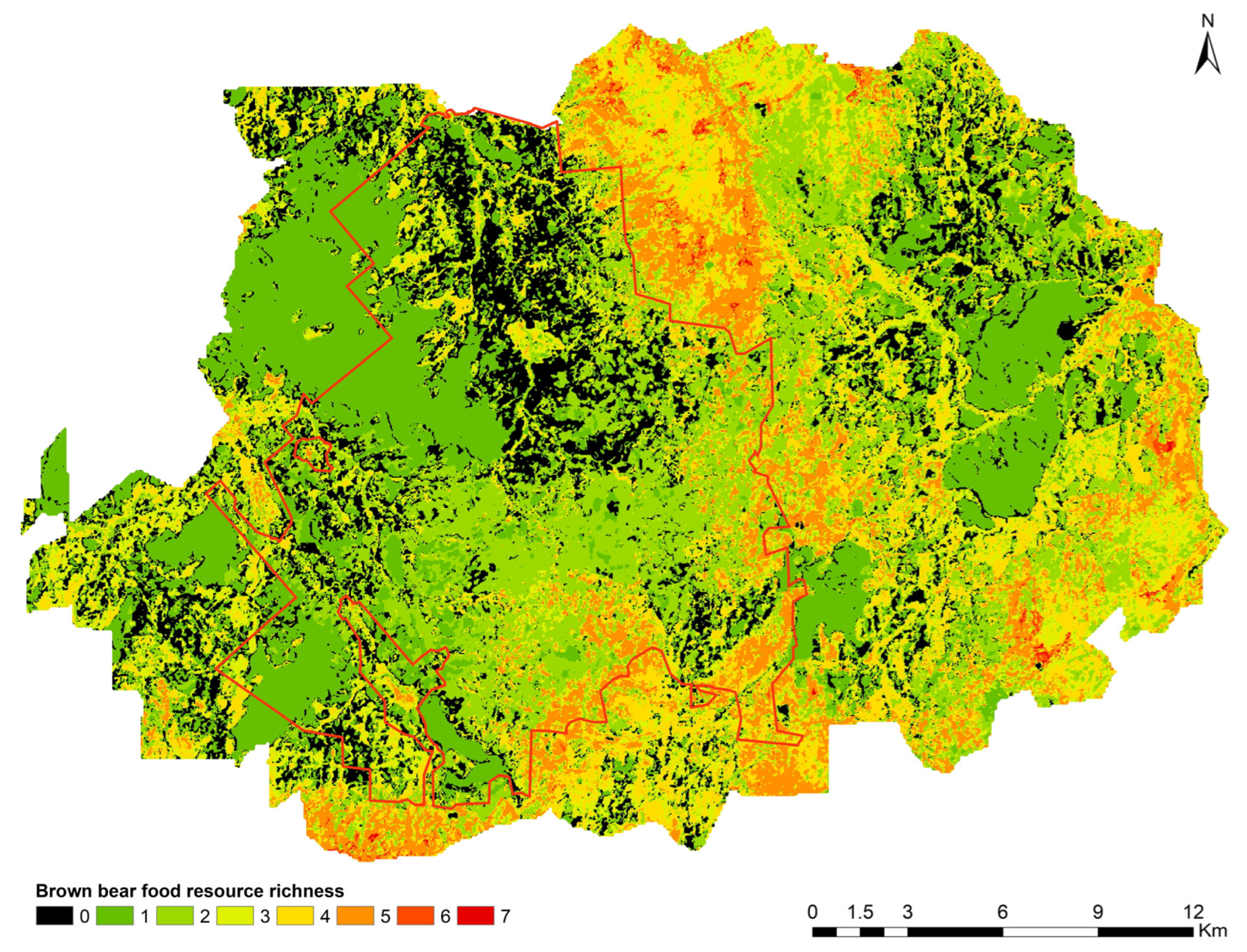
Status of the Area and
Proportion of Pixels
Number of Food Resources per Pixel in the Map of Figure 7
01234567
CFNR core area (%)21.2425.9932.109.556.204.840.090
CFNR buffer zone (%)11.4722.8020.1816.2216.4911.870.810.16
Publisher’s Note: MDPI stays neutral with regard to jurisdictional claims in published maps and institutional affiliations.

