Abstract
The sweet chestnut (Castanea sativa Mill.) is an important species of European trees, studied for both ecological and economic reasons. Its cultivation in the Italian peninsula can be linked to the Roman period and has been documented, especially in the Tuscan region, for centuries. We sampled 131 grafted trees from three separate areas to determine the genetic variability between populations and assess genetic identity for different varieties of trees, which is useful for future breeding programs and propagation efforts. Molecular analyses were performed using eight microsatellite loci. A total of 98 alleles was detected with an average of 12.3 alleles per locus. We found high levels of genetic diversity within the varieties of the same area, ranging between He = 0.682–0.745. Of the eight loci, seven were found to be at Hardy-Weinberg equilibrium. (FST values Differentiation between cultivation areas was significant between 0.052–0.147) with the two Southern Tuscan areas showing the closest relationship as also indicated by Bayesian inference of the population structure, which revealed the existence of three ancestral gene pools of origin. Demographic events were detected by a coalescent-based approximate Bayesian computation in two of the homogeneous clusters. This work is a step forward for the conservation of this iconic species, albeit at a regional level, as chestnut varieties have never received the full attention of breeders.
1. Introduction
Edible sweet chestnuts (Castanea sativa Mill.) have been cultivated for centuries representing an important food resource for rural populations in mountain regions of many countries [1]. The tree is the only European species of the genus Castanea (Fagaceae; x = 12, 2n = 24, [2]) and is considered to be native to Asia, expanding later into the Balkan region during the middle Eocene. After its introduction in Italy by the Greeks [3] the rapid expansion towards the present areas of cultivation occurred, mainly, during the Roman period [4,5]. Chestnut trees have at least a 2000 year long cultivation history in Italy, however Italian chestnut varieties never received the full attention of breeders and the efforts made to genetically characterise the trees have been sporadic at best. Due to the dual role of the chestnut as both a staple food source and wood producer, the chestnut has undergone natural and artificial selection leading to the differentiation of the product and wide range of germplasm varieties present today [6].
Many studies have reported the assessment of genetic variability and structuring of chestnuts throughout Europe, mainly by the use of SSRs, due to the renewed importance of chestnut trees for ecological and economic reasons as can also be demonstrated by the several available genetic maps. The species is also studied for its interspecific crosses [7,8,9], which allow us to identify homeologous chromosomal regions and therefore, regions possibly harbouring adaptive traits within the Fagaceae family. Mattioni et al. [10] studied 31 chestnut populations from Eastern (Greece and Turkey) and Western Europe, to test for the hypothesised presence of refugia during the last glacial maximum based on pollen records [11] and for differences between the eastern and western gene pools, suggesting that, in general, human intervention played an important role in establishing the current genetic structure of sweet chestnut as suggested by Conedera et al. [4]. An important corollary of this is that all conservation strategies should consider all levels of biodiversity and, in particular, intraspecific genetic variation, a key factor for a species’ ability to cope with environmental stress. Therefore, it becomes of importance to assess the genetic variability of the chestnut in natural populations as well as in cultivated varieties. This was done with isozymes and SSRs [12,13,14,15,16,17], with much emphasis on the Italian chestnut germplasm, which includes hundreds of cultivars, revealing a very complex varietal panorama. According to Mattioni et al. [18], the results of these studies suggest that sweet chestnut populations still contain higher diversity than varieties. Using microsatellite markers, a considerable genetic uniformity among “Marrone-type” [19,20] was highlighted as opposed to a high genetic diversity among Italian and European “chestnut-type” cultivars [3].
Sweet chestnut stands in Italy have been greatly reduced in size and scope in the last decades, because of social and economic factors. The very task of managing a chestnut wood is being forgotten. In the wake of a new consciousness about the conservation of genetic resources, an assessment of the resources at hand will become of increased importance. The aim of this work was therefore to characterise the genetic structure of sweet chestnut trees collected in three different areas of Tuscany: Garfagnana, Colline Metallifere, and Amiata. These areas are greatly informative as cultivations have been documented in the region for several centuries, albeit always based on a local geographical scale. The three areas are geographically close but chestnut trees are not present in between. In addition, a confounding effect is represented by the fact that the 102 trees sampled are known by the local growers with 39 local names, only one of which was present in all three areas and four were present in two areas. Therefore, a second aim of the research is to assess the genetic identity of a representative set of traditional chestnut varieties from a local germplasm, to pave the road for future breeding programs, varietal identification by genetic markers and propagation of the most relevant varieties for commercial purposes.
2. Materials and Methods
2.1. Study Area
The last survey on chestnut cultivation performed by Regione Toscana identified a total coverage of 32,336 hectares, half of those being abandoned. The three studied areas (Figure 1) are representative of the three major sweet chestnut production districts in Tuscany. Among these, the Garfagnana area is the most important in terms of chestnut presence and biodiversity. At the beginning of the 1900s, more than 2000 productive hectares were present in this area and now only about 3000 remain cultivated. No information is available about chestnut distribution in the other two areas, which both display a progressive reduction of cultivation and loss of biodiversity in common. In this study, we analysed grafted trees chosen on the basis of the given local names of the respective variety, reported in Supplementary Table S1. Many of these local names are related to toponyms and are not translatable, but it will suffice to say that the root “marron” refers to all Marrone-like varieties. When this root is not present, the variety refers to “non-Marrone” chestnuts, which in Italy are also grafted. Note that, although all trees were grafted, grafting in the studied area does not follow a regular pattern, instead being been based on the local preferences for a given fruit type. Chestnut trees were sampled mostly within germplasm collections. These local collections were established in the recent past by grafting selected vegetal material on seedlings or naturally growing plants. The history of each plant was well known by the curators of the collections. We surveyed the area with the head of the growers associations and interviewed all the owners of the mother plants. Samples were then collected from plants that were grafted by the owner or one of the original ancestors. The graft point was recognizable by a scar in the trunk or a bulge in correspondence of the union between rootstock and scion, located one to two metres from the ground (Supplementary Figure S1). Samples were collected only from the upper part of the canopy above the graft point of each plant. The same method was used to collect samples from the mother plants outside the collections.
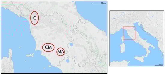
Figure 1.
Location of the study area (Tuscany, Italy) and spatial distribution of the population nuclei. G = Garfagnana; CM = Colline Metallifere; MA = Monte Amiata.
2.2. Genetic Analysis
Chestnut trees were sampled within local germplasm collections or well recognised local mother plants in collaboration with growers’ associations. Total genomic DNA was extracted from 100 mg of fresh tissue using a modified Doyle and Doyle [21] method. Molecular analysis was performed with eight microsatellite markers, chosen also on the basis of their position (different linkage groups) on the available genetic maps [7]. All polymerase chain reactions (PCRs) with the DNA extracted from the accessions were performed on a Mastercycler Gradient (Eppendorf AG, Hamburg, Germany) in 25 μL volume containing 5 μL of DNA (10 ng/μL) and 20 μL mix. The eight primer pairs; CsCAT1, CsCAT3, CsCAT6, CsCAT16, CsCAT17 [22], EMCs22, EMCs25, and EMCs38 [23] were labelled with 6FAM, HEX, and NED fluorescent dyes for multiplexed genotyping (Table 1). Cycling conditions were the same for all loci. Initially, DNA was denatured for 3 min at 94 °C followed by 35 cycles of 94 °C for 30 s, annealing temperature (Ta) for 30 s, and 72 °C for 30 s. A final 8 min extension at 72 °C was included. Allele sizing was performed by the GeneMarker program after sequencing on a MegaBACE™ 500 capillary sequencer (GE Healthcare).

Table 1.
Primer sequences and annealing temperatures (Ta) for the eight SSRs used in this study.
Allele frequencies, and observed and expected heterozygosity were estimated at each locus, as as was the polymorphism information content (PIC), which was calculated with Cervus 3.0.7 [23]. The estimated frequency of null alleles for each locus was calculated using the Micro-checker software under the Brookfield 1 model [24]. All subsequent analyses were done using Genetix 4.05.2 [25]. Weir and Cockerham’s [26] estimators of F-statistics were applied to analyse genetic diversity both within and among populations. In particular, FIS and FST were calculated to assess the extent of total genetic variation caused by any departure from Hardy-Weinberg equilibrium at the population level and differentiation among populations, respectively. The deviation of FIS from zero was tested for all loci in all populations under the null hypothesis of Hardy-Weinberg equilibrium by a permutation test based on 1000 replications. Nei’s genetic distance [27] was calculated for pairwise comparisons of populations, under an infinite-allele-model. Principal coordinate analysis (PCoA) was performed based on those pairwise genetic distances between the individuals.
To investigate the presence of genetic structuring in the studied populations, we used the Bayesian clustering analyses implemented in the program STRUCTURE 2.3.1 [28]. First, we determined the most likely number of ancestral gene pools, K, based on nuclear microsatellite genotypes. This was carried out via the ΔK method developed by Evanno et al. [29], using Harvester [30]. Ten independent runs were performed for each K between one and six, with a “no admixture” model using prior population information with LOCPRIOR [31], 50,000 MCMC iterations and a 10,000-iteration burn-in period.
The likelihood of the 10 runs was averaged using CLUMPAK [32] an online resource based on the LargeKGreedy algorithm of CLUMPP with 2000 replicates [33] and shown graphically by DISTRUCT [34].
2.3. Demography
The demographic history was investigated through a coalescent-based approximate Bayesian computation as implemented in the DIYABC version 2.1.0 algorithm [35] on the ancestral genetic clusters identified by STRUCTURE.
To estimate the demographic parameters, we followed the strategy used by [36]: first, we used a model so that both present and past population sizes were allowed to vary freely. This was done to ensure that every possible demographic event could be detected. Next, a model allowing a single event of contraction and a single event of expansion of the demographic size was used. Data obtained from the two models were compared to confirm that a scenario with population size change was supported.
Posterior distributions were obtained for three composite parameters: population diversity parameters N0µ0 (present), N1µ1 (past), and ratio r0 = N0µ0/N1µ1, plus all single parameters. Posterior parameter distributions were estimated under the best scenario using a linear regression on the 1% closest simulations and applying a logit transformation to parameter values [31,32,33,34,35]. We focused on r0 because it correctly represents ratios of effective population sizes [35]. Indeed, if we assume constant mutation rates over time (µ0 = µ1 = µ), we obtain:
the ratio of present-to-past effective population sizes. Details about parameter estimation are presented in Supplementary Materials.
r0 = N0µ0/N1µ1 = N0µ/N1µ = N0/N1
3. Results
3.1. Genetic Diversity
We genotyped eight SSR loci in 102 chestnut individuals from three geographic regions. We found elevated levels of genetic diversity as indicated by the observed mean heterozygosity (Ho) values ranging from 0.684 (G) to 0.749 (MA) and by the expected mean heterozygosity (He) values ranging from 0.682 (G) to 0.745 (MA). At the single locus level, Ho varied from 0.029 (locus EMC25, G region) to 0.951 (locus CsCAT17, CM region)) and He from 0.371 (locus EMC25, G region) to 0.891 (locus EMC38, CM region). A total of 98 alleles was detected with a mean of 12.3 alleles per locus. The total number of alleles per locus ranged from 8 (loci CsCAT1 and CsCAT16) to 21 (locus EMC38). The number of alleles (averaged over loci) for each geographical region ranged from 6.9 for G to 9.3 for CM. The very same locus, EMC25, which displayed by far the lowest variability in the dataset was found at Hardy-Weinberg disequilibrium because of an excess of homozygotes in all three populations; the other eight significant FIS values, four positive, four negative, were scattered across populations (see Table 2). All SSRs used had PIC values > 0.7, thus being very informative according to the criterion used in Alessandri et al. [3] (See Table 2). Null alleles were predicted for the CsCAT3 and EMC25 loci only. Taking these into account did not modify the overall heterozygosity estimates (0.796 and 0.583 respectively).
Table 2.
Expected (He) and observed (Ho) heterozygosity are reported for each locus and each population, together with the mean across all loci. FIS is also reported for all loci and as an overall estimate for each population (last row). Values of FIS in bold are significantly different from zero (p < 0.05), indicating Hardy–Weinberg disequilibrium.
3.2. Genetic Differentiation and Distance
The overall genetic differentiation amongst populations was significant: about 10% (FST = 0.105, confidence interval at 95% is 0.048 < FST < 0.176) of the total genetic variation can be attributed to differentiation amongst regions. When doing pairwise comparisons, FST values were significant again: from highest to lowest, 0.147 (G vs. MA), 0.116 (G vs. CM), and 0.052 (CM vs. MA). The same trend was found when we estimated the genetic distance amongst populations by means of Nei’s genetic distance; the relative distances were: 0.598 (G vs. MA), 0.412 (G vs. CM), and 0.188 (CM vs. MA). The significance of both FST and Nei’s D values was tested by a permutation procedure with 1000 replications. Both genetic differentiation and distances point to a closer relationship between the two regions of Southern Tuscany. In graphical form, this is displayed by the Principal Coordinate Analysis (PCoA) graph (Figure 2), where each tree is represented in a Euclidean space with coordinates based on the genetic distances, which confirms the standing apart of the G region. Only a few trees display the same genotype for all eight SSRs, as expected given the random basis of grafting in these regions.
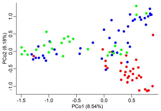
Figure 2.
Principal Coordinate Analysis (PCoA). Each chestnut tree is represented by a dot in a two-dimensional space represented by the two first Principal Coordinates, which explain, respectively, 8.54% and 6.18% of the total variation. The Euclidean distance between trees is based on their genotypic differences. Different regions are represented by different colours: red = Garfagnana (G), blue = Colline Metallifere (CM), green = Monte Amiata (MA). The red dot on the extreme left is tree G17 (see text for details).
3.3. Structure Analysis
The population structure in the three populations was investigated by the Bayesian procedure implemented in the software STRUCTURE [28]. First, we estimated the most likely number of clusters (K), or homogeneous gene pools, to have originated in the present populations, based on ΔK, the second-order rate of change of the likelihood function with respect to K [29]. We obtained a sharp signal at K = 3 (Supplementary Figure S2), thus indicating that three gene pools shaped the genetic structure of the populations analysed. Based on K = 3, the final proportion of each of the three hypothetical gene pools present in each population and each tree was obtained and the results are shown in Table 3 and in Figure 3. The trees of the G region derived almost of the entirety of their genome (0.96) from a single gene pool of origin, which is different from the ones mainly originating the CM and MA gene clusters, which were not so clearly structured. In particular, the latter presented an almost equal admixture of the two genetic origins.
Table 3.
Analysis of population structure according to a Bayesian clustering method. The populations studied derive their genetic structure from three inferred gene pools of origin. The proportion of membership of each inferred population in the populations studied is indicated. The main contribution is in bold.
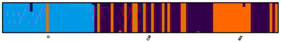
Figure 3.
Genetic structure of the studied chestnut trees as inferred by Bayesian clustering of SSR genotypes at K = 3. Each vertical bar represents a single tree and the proportion of membership to a genetic pool is indicated by the different colours.
The same findings are confirmed when we look at the genetic composition at the single tree level (Figure 3): the trees of the G region appeared to be genetically uniform, with the exception of tree #17, which appeared to belong to a “Southern Tuscan” gene pool. This was confirmed by an ad hoc investigation about the provenance of the tree thus, again confirming the ability of Bayesian analysis to trace back the genetic origin of single individuals.
An interesting finding was the good correspondence between the genetic clusters detected and the trees with similar variety local names. In fact, whereas for the Garfagnana trees a single gene pool of origin was detected, trees from the other two regions showed origins resulting from two different pools (purple and orange in Figure 3). However, when grouped according to the genetic pool of origin, trees with similar local names clustered together, as shown in Supplementary Table S2.
3.4. Demographic History
We analysed the homogeneous genetic clusters obtained by STRUCTURE, where the first cluster corresponded to the Garfagnana site, with the exception of tree #17, and the other two clusters represented combinations of the trees from the Colline Metallifere and Monte Amiata sites. ABC detected a variation in Ne for all considered genetic clusters: A contraction scenario was the most likely for Clusters 1 and 3 (red and blue, respectively, in Figure 3), as indicated by r0 < 1 (Table 4), whereas an expansion scenario was the most likely for Cluster 2. The size of demographic change varied roughly between a 25-fold contraction for Cluster 1, a nine-fold contraction for Cluster 3 and a two-fold expansion for Cluster 2. In a second approach, we compared, by a logistic approach, the respective probabilities of a contraction or an expansion episode for each of the homogeneous gene clusters. The contraction episodes were confirmed for Clusters 1 and 3 by a relative p of 0.99 and 0.95, respectively, against the p of an expansion. The expansion of Cluster 2 was confirmed, but with a lower probability (p = 0.57) over a contraction [37].
Table 4.
Parameter estimation for the Approximate Bayesian Computation (ABC) modelling with free population size variation. All parameter values are provided with their credible interval at 95%. T: Median of the time to demographic event; N0µ, N1µ: median of (respectively) present and past diversity index, with N the effective population size and μ the mutation rate; r0: median of the ratio N0µ/N1µ. The density distributions obtained for the posterior estimates of the ratio (r0) of present (N0μ) and past (N1μ) diversity population indexes are also reported in Supplementary Figure S3.
4. Discussion
Chestnut trees have at least a 2000-year-long cultivation history in Italy, however Italian chestnut varieties have never received the full attention of breeders and the efforts made to genetically characterise the trees have been sporadic at the best. This is part In Italy, and other countries, a long history of forestry practitioners not relying on the evidence coming from genetics [38] has been evident and affected chestnut trees, too. However, all conservation strategies should consider all levels of biodiversity and, in particular, intraspecific genetic variation, a key factor for a species’ ability to cope with environmental stress. In this work, we focused on three areas of Tuscany, one of the regions where chestnuts have been an important staple food for many centuries. More than 100 trees were genotyped for eight SSRs, unveiling high values of genetic diversity, both Ho and He in the range of 0.68–0.75. These values are very similar to those obtained in Mattioni et al., [39] (He in the range 0.58–0.80) for several chestnut populations of central Italy by means of six SSRs representing a subset of our eight. Because said work suggested that the high levels of genetic diversity found in Central Italy indicate that this area was a refuge for sweet chestnut, we cannot rule out the possibility that in the areas studied in our work some remnants of old chestnut trees can also be found. Moreover, values of expected heterozygosity are in agreement with those obtained from other European chestnut populations [40,41], which is particularly evident in the work of Lusini et al. [42], where six populations from Bulgaria were assessed using eight SSRs and whose He values were in the range of 0.67–0.80.
Because of an increasing attention to the provenance of fruits by the public and stakeholders alike, it is also of importance to define whether different “varieties” are also genetically differentiated. In fact, many varietal definitions are given solely on a historical basis. This was also a starting point of our study, because in the studied regions grafting was done for the production of fruits with characteristics chosen by the farmers and not yet determined by marketing strategies. This is reflected in the very large number of local names for trees that appear to be identical; however, these practices allowed for a large amount of genetic diversity to be maintained, as also indicated by the fact that only a few trees have the same genotype (therefore grafted from the same material) at least for the relatively few number of studied markers.
We studied three distinct regions; two of these were close to each other, and, not surprisingly, revealed lower FST values and a partial overlap of their genetic structure. The trees belonging to the third region (Garfagnana, in Northern Tuscany) were clearly differentiated and showed an origin from a different gene pool. This situation mirrors, at a small geographic scale, the strong geographical structure found across Europe in wild populations from Turkey, Greece, Italy and Spain [10], and confirmed by the two main genetic clusters of origin found in wild chestnut in Spain, Italy and Greece [35], and by the three genetic clusters identified in wild and natural populations [43]. More recently, a large study focused on the Italian and Iberian peninsulas and based on 16 SSRs confirmed that these two genetic clusters are clearly separated [3]. Our work is not aimed at making inferences about the biogeographical history of chestnut, but the strong genetic structure agrees with evidence of establishment originating from the Last Glacial Maximum refugia, one of which could have been localised in Central Italy [44].
Under the point of view of conservation of genetic resources, our results are of interest because of the possibility to detect differences in the chestnut germplasm also at a small geographical scale and because of the implications in the face of global climate change (GCC). In fact, chestnut is a species sensitive to progressive climate warming and shortage of water resources, because of its requirements in terms of continuous water supply and soil moisture.
The potential of a species to adapt to different environmental conditions depends on: i—the level of genetic diversity of a population and ii—the extent of migration and gene flow between populations. When gene flow and dispersal are limited, as could be the case with established populations such as in chestnut varieties used for fruit production, environmental changes can lead to demographic shifts that can be deleterious, especially in small populations. Thus, besides estimating standing genetic variation essential for adaptation, genetic data can also provide interesting information on species (“variety”) demography and population size Ne. A first attempt at detecting variations in the past demography of the genetic clusters obtained was made by coalescent modelling coupled with ABC, finding that all clusters possibly underwent a change in their population size in the past. The ratios of present-to-past diversity parameters r0 were reliably estimated, as indicated by the narrow credibility intervals and peaked posterior distributions (Table 4, Supplementary Figure S3), suggesting that demographic transitions were correctly captured by the model and the data. However, the real size of observed demographic changes is to be considered as a relative one and not an absolute value.
That said, the most immediate explanation of this is anthropogenic pressure in the geographic proximity of the varieties studied and/or a decrease in interest in sweet chestnut cultivation due to more remunerative agricultural possibilities. We cannot rule out the possibility of purely neutral events, leading to random fluctuations of the demographic size [45]. However, it is important to estimate these demographic parameters, because they can serve as estimators of the adaptive potential of a population/variety to cope with environmental changes [46].
We can see how global climate change is negatively impacting chestnut cultivations. It is therefore imperative to study genetic variability even at a local level to identify adaptive traits that could help with species preservation, as has been done in other species [47,48], and also in chestnut [49]. Genes involved in adaptation have been linked to precipitations, indicating that drought resistance plays a role in species survival in given areas. In conclusion, our work will be of great use in the future as it lays the foundations for the development of specific markers that could be used to identify adaptive genetic variation and further develop SNPs, as was commenced by Larue et al. [50].
Supplementary Materials
The following supporting information can be downloaded at: https://www.mdpi.com/article/10.3390/f13070967/s1. Parameter estimate. Details on the procedure used to estimate the demographic parameters used. Figure S1. Grafted chestnut tree. The circle highlights the scar where the grafting occurred, roughly one meter above the ground, Figure S2. Graphical ∆K representation of the estimated probability of data for each K-value from K = 2 to K = 9. Admixture model with LOCPRIOR, 50,000 MCMC iterations and a 10,000 iterations burn-in period, Figure S3. Density distributions obtained by the ABC approach of posterior estimates of the ratio (r0) of present (N0μ) and past (N1μ) diversity population index. Clusters 1, 2 and 3 correspond to the homogeneous genetic clusters obtained by STRUCTURE analysis (see text for details). Dashed lines are prior distributions, the full red lines are posterior distributions, Table S1. Local names of trees sampled for this work, ordered by area. G = Garfagnana, CM = Colline Metallifere, MA = Monte Amiata, Table S2. Local names of trees sampled for this work, ordered by gene cluster of provenance after analysis by STRUCTURE. “Marroni” trees are present in all clusters. References [51,52,53,54] are cited in the supplementary materials.
Author Contributions
C.C. planned the research and acquired some funding; G.B., C.C. and M.C. carried out the formal analysis of the data; G.L., C.C. and G.B. drafted the manuscript. All authors have read and agreed to the published version of the manuscript.
Funding
This research was partially funded by grant FAR 2020 of University of Insubria to G.B.
Institutional Review Board Statement
Not applicable.
Informed Consent Statement
Not applicable.
Data Availability Statement
Not applicable.
Conflicts of Interest
The authors declare no conflict of interest.
References
- Neri, L.; Dimitri, G.; Sacchetti, G. Chemical composition and antioxidant activity of cured chestnuts from tree sweet chestnut (Castanea sativa Mill.) ecotypes from Italy. J. Food Compos. Anal. 2010, 23, 23–29. [Google Scholar] [CrossRef]
- Jaynes, R.A. Chestnut chromosomes. For. Sci. 1962, 13, 372–377. [Google Scholar]
- Alessandri, S.; Cabrer, A.M.R.; Martìn, M.A.; Mattioni, C.; Pereira-Lorenzo, S.; Dondini, L. Genetic characterization of Italian and Spanish wild and domesticated chestnut tress. Sci. Hortic. 2022, 295, 110882. [Google Scholar] [CrossRef]
- Conedera, M.; Krebs, P.; Tinner, W.; Pradella, M.; Torriani, D. The cultivation of Castanea sativa (Mill.) in Europe, from its origin to its diffusion on a continental scale. Veg. Hist. Archaeobot. 2004, 13, 161–179. [Google Scholar] [CrossRef]
- Zohary, D.; Hopf, M. Domestication of Plants in the Old World; Claredon Press: Oxford, UK, 1988. [Google Scholar]
- Casoli, M.; Mattioni, C.; Cherubini, M.; Villani, F. A genetic linkage map of European chestnut (Castanea sativa Mill.) based on RAPD, ISSR and isozyme markers. Theor. Appl. Genet. 2001, 102, 1190–1199. [Google Scholar] [CrossRef]
- Barreneche, T.; Casasoli, M.; Russell, K.; Akkak, A.; Meddour, H.; Plomion, C.; Villani, F.; Kremer, A. Comparative mapping between Quercus and Castanea using simple-sequence repeats (SSRs). Theor. Appl. Genet. 2004, 108, 558–566. [Google Scholar] [CrossRef]
- Staton, M.; Zhebentyayeva, T.; Olukolu, B.; Fang, G.C.; Nelson, D.; Carlson, J.E.; Abbott, A.G. Substantial genome synteny preservation among woody angiosperm species: Comparative genomics of Chinese chestnut (Castanea mollissima) and plant reference genomes. BMC Genom. 2015, 16, 744. [Google Scholar] [CrossRef]
- Santos, J.; Antorrena, G.; Freire, M.S.; Pizzi, A.; Gonzàles-Alvàrez, J. Environmentally friendly wood adhesives based on chestnut (Castanea sativa) shell tannins. Eur. J. Wood Wood Prod. 2017, 75, 89–100. [Google Scholar] [CrossRef]
- Mattioni, C.; Martin, M.A.; Pollegioni, P.; Cherubini, M.; Villani, F. Microsatellite markers reveal a strong geographical structure in European populations of Castanea sativa (Fagaceae): Evidence for multiple glacial refugia. Am. J. Bot. 2013, 100, 951–961. [Google Scholar] [CrossRef]
- Huntley, B.; Birks, H.J.B. An Atlas of Past and Present Pollen Maps for Europe: 0–13,000 Years Ago; Cambridge University Press: Cambridge, UK, 1983; p. 688. [Google Scholar]
- Fineschi, S.; Malvolti, M.E.; Morganti, M.; Vendramin, G.G. Allozyme variation within and among cultivated varieties of sweet chestnut (Castanea sativa). Can. J. For. Res. 1994, 24, 1160–1165. [Google Scholar] [CrossRef]
- Villani, F.; Pigliucci, M.; Cherubini, M. Evolution of Castanea sativa Mill. in Turkey and Europe. Genet. Res. 1994, 63, 109–116. [Google Scholar] [CrossRef]
- Villani, F.; Sansotta, A.; Cherubini, M.; Cesaroni, D.; Sbordoni, V. Genetic structure of natural population of Castanea sativa in Turkey: Evidence of a hybrid zone. J. Evol. Biol. 1999, 12, 233–244. [Google Scholar] [CrossRef]
- Galderisi, U.; Cipollaro, M.; Bernardo, G.; Masi, L.; Galano, G.; Cascino, A. Molecular typing of Italian sweet chestnut cultivars by random amplified polymorphic DNA analysis. J. Hortic. Sci. Biotech. 1998, 73, 259–263. [Google Scholar] [CrossRef]
- Boccacci, P.; Akkak, A.; Marinoni, D.; Bounous, G.; Botta, R. Typing european chestnut (Castanea sativa Mill.) cultivars using oak simple sequence repeat markers. HortScience 2004, 39, 1212–1216. [Google Scholar] [CrossRef]
- Botta, R.; Akkak, A.; Guaraldo, P.; Bounous, G. Genetic characterization and nut quality of chestnut cultivars from Piemonte (Italy). Acta Hortic. 2005, 693, 395–401. [Google Scholar] [CrossRef]
- Mattioni, C.; Cherubini, M.; Micheli, E.; Villani, F.; Bucci, G. Role of domestication in shaping Castanea sativa genetic variation in Europe. Tree Genet. Genomes 2008, 4, 563–574. [Google Scholar] [CrossRef]
- Martin, M.A.; Mattioni, C.; Cherubini, M.; Taurchini, D.; Villani, F. Genetic characterization of traditional chestnut varieties in Italy using microsatellites (simple sequence repeats) markers. Ann. Appl. Biol. 2010, 157, 37–44. [Google Scholar] [CrossRef]
- Alessandri, S.; Krznar, M.; Ajolfi, D.; Ramos Cabrer, A.M.; Pereira-Lorenzo, S.; Dondini, L. Genetic Diversity of Castanea sativa Mill. Accessions from the Tuscan-Emilian Apennines and Emilia Romagna Region (Italy). Agronomy 2020, 10, 1319. [Google Scholar] [CrossRef]
- Doyle, J.J.; Doyle, J.L. A rapid DNA isolation procedure for small quantities of fresh leaf tissue. Phytochem. Bull. 1987, 19, 11–15. [Google Scholar]
- Marinoni, D.; Akkak, A.; Bounous, G.; Edwards, K.J.; Botta, R. Development and characterization of microsatellite markers in Castanea sativa (Mill.). Mol. Breed. 2003, 11, 127–136. [Google Scholar] [CrossRef]
- Kalinowski, S.T.; Taper, M.L.; Marshall, T.C. Revising how the computer program CERVUS accommodates genotyping error increases success in paternity assignment. Mol. Ecol. 2007, 16, 1099–1106. [Google Scholar] [CrossRef] [PubMed]
- Buck, E.J.; Hadonou, M.; James, C.J.; Blakesley, D.; Russell, K. Isolation and characterization of polymorphic microsatellites in European chestnut (Castanea sativa Mill.). Mol. Ecol. Notes 2003, 3, 239–241. [Google Scholar] [CrossRef]
- Belkhir, K.; Borsa, P.; Chikhi, L.; Raufaste, N.; Bonhomme, F. GENETIX 4.02, Logiciel Sous WindowsTM Pour la Génétique des Populations; Laboratoire Génome, Population Interaction, CNRS; Université de Montpellier II: Montpellier, France, 1996. [Google Scholar]
- Weir, B.S.; Cockerham, C.C. Estimating F-statistics for the analysis of population structure. Evolution 1984, 38, 1358–1370. [Google Scholar] [PubMed]
- Nei, M. Estimation of average heterozygosity and genetic distance from a small number of individuals. Genetics 1978, 89, 583–590. [Google Scholar] [CrossRef] [PubMed]
- Pritchard, J.K.; Stephens, M.; Donnelly, P. Inference of population structure using multilocus genotype data. Genetics 2000, 155, 945–959. [Google Scholar] [CrossRef] [PubMed]
- Evanno, G.; Regnaut, S.; Goudet, J. Detecting the number of clusters of individuals using the software STRUCTURE: A simulation study. Mol. Ecol. 2005, 14, 2611–2620. [Google Scholar] [CrossRef]
- Dent, E.A.; vonHoldt, B.M. STRUCTURE HARVESTER: A website and program for visualizing STRUCTURE output and implementing the Evanno method. Conserv. Genet. Res. 2012, 4, 359–361. [Google Scholar]
- Hubisz, M.J.; Falush, D.; Stephens, M.; Pritchard, J.K. Inferring weak population structure with the assistance of sample group information. Mol. Ecol. Resour. 2009, 9, 1322–1332. [Google Scholar] [CrossRef]
- Kopelman, N.M.; Mayzel, J.; Jakobsson, M.; Rosenberg, N.A.; Mayrose, I. CLUMPAK: A program for identifying clustering modes and packaging population structure inferences across K. Mol. Ecol. Res. 2015, 15, 1179–1191. [Google Scholar] [CrossRef]
- Jakobsson, M.; Rosenberg, N.A. CLUMPP: A cluster matching and permutation program for dealing with label switching and multimodality in analysis of population structure. Bioinformatics 2007, 23, 1801–1806. [Google Scholar] [CrossRef]
- Rosenberg, N.A. DISTRUCT: A program for the graphical display of population structure. Mol. Ecol. Notes 2004, 4, 137–138. [Google Scholar] [CrossRef]
- Cornuet, J.M.; Santos, F.; Beaumont, M.A. Inferring population history with DIY ABC: A user-friendly approach to approximate Bayesian computation. Bioinformatics 2008, 24, 2713–2719. [Google Scholar] [CrossRef]
- Barthe, S.; Binelli, G.; Hérault, B.; Scotti-Saintagne, C.; Sabatier, D.; Scotti, I. Tropical rainforests that persisted: Inferences from the Quaternary demographic history of eight tree species in the Guiana shield. Mol. Ecol. 2017, 26, 1161–1174. [Google Scholar] [CrossRef]
- Beaumont, M.A.; Zhang, W.; Balding, D.J. Approximate Bayesian computation in population genetics. Genetics 2002, 162, 2025–2035. [Google Scholar] [CrossRef]
- Bowman, J.; Greenhorn, J.E.; Marrotte, R.R.; McKay, M.M.; Morris, K.Y.; Mrentice, M.B.; Wehtje, M. On application of landscape genetics. Conserv. Genet. 2016, 17, 753–760. [Google Scholar] [CrossRef]
- Mattioni, C.; Martin, M.A.; Chiocchini, F.; Cherubini, M.; Gaudet, M.; Pollegioni, P.; Velichkov, I.; Jarman, R.; Chambers, F.M.; Paule, L.; et al. Landscape genetics structure of European sweet chestnut (Castanea sativa Mill): Indications for conservation priorities. Tree Genet. Genomes 2017, 13, 39. [Google Scholar] [CrossRef]
- Poljak, I.; Idžojtić, M.; Šatović, Z.; Ježić, M.; Ćurković-Perica, M.; Simovski, B.; Acevski, J.; Liber, Z. Genetic diversity of the sweet chestnut (Castanea sativa Mill.) in Central Europe and the western part of the Balkan Peninsula and evidence of marron genotype introgression into wild populations. Tree Genet. Genomes 2017, 13, 18. [Google Scholar] [CrossRef]
- Cuestas, M.I.; Mattioni, C.; Martin, L.M.; Vargas-Osuna, E.; Cherubini, M.; Martin, M.A. Functional genetic diversity of chestnut (Castanea sativa Mill.) populations from southern Spain. For. Syst. 2017, 26, eSC06. [Google Scholar] [CrossRef]
- Lusini, I.; Velichkov, I.; Pollegioni, P.; Chiocchini, F.; Hinkov, G.; Zlatanov, T.; Cherubini, M.; Mattioni, C. Estimating the genetic diversity and spatial structure of Bulgarian Castanea sativa populations by SSRs: Implications for conservation. Conser. Genet. 2014, 15, 283–293. [Google Scholar] [CrossRef]
- Fernàndez-Cruz, J.; Fernàndez-Lòpez, J. Genetic structure of wild sweet chestnut (Castanea sativa Mill.) populations in northwest of Spain and their differences with other European stands. Conserv. Genet. 2016, 17, 949–967. [Google Scholar] [CrossRef]
- Martin, M.A.; Mattioni, C.; Molina, J.R.; Alvarez, J.B.; Cherubini, M.; Herrera, M.A.; Villani, F.; Martin, L.M. Landscape genetic structure of chestnut (Castanea sativa Mill.) in Spain. Tree Genet. Genomes 2012, 8, 127–136. [Google Scholar] [CrossRef]
- Hubbell, S.P. The Unified Neutral Theory of Biodiversity and Biogeography; Princeton University Press: Princeton, NJ, USA, 2001. [Google Scholar]
- Exposito-Alonso, M.; Vasseur, F.; Ding, W.; Wang, G.; Burbano, H.A.; Weigel, D. Genomic basis and evolutionary potential for extreme drought adaptation in Arabidopsis thaliana. Nat. Ecol. Evol. 2018, 2, 352–358. [Google Scholar] [CrossRef]
- Di Pierro, E.A.; Mosca, E.; González-Martínez, S.C.; Binelli, G.; Neale, D.B.; La Porta, N. Adaptive variation in natural Alpine populations of Norway spruce (Picea abies [L.] Karst) at regional scale: Landscape features and altitudinal gradient effects. For. Ecol. Manag. 2017, 405, 350–359. [Google Scholar] [CrossRef]
- Yücedağ, C.; Müller, M.; Gailing, O. Morphological and genetic variation in natural populations of Quercus vulcanica and Q. frainetto. Plant Syst. Evol. 2021, 307, 8. [Google Scholar] [CrossRef]
- Castellana, S.; Martin, M.Á.; Solla, A.; Alcaide, F.; Villani, F.; Cherubini, M.; Neale, D.; Mattioni, C. Signatures of local adaptation to climate in natural populations of sweet chestnut (Castanea sativa Mill.) from southern Europe. Ann. For. Sci. 2021, 78, 27. [Google Scholar] [CrossRef]
- Larue, C.; Guichoux, E.; Laurent, B.; Barreneche, T.; Robin, C.; Massot, M.; Delcamp, A.; Petit, R.J. Development of highly validated SNP markers for genetic analyses of chestnut species. Conserv. Genet. Resour. 2021, 13, 383–388. [Google Scholar] [CrossRef]
- Zhivotovsky, L.A.; Feldman, M.W.; Grishechkin, S.A. Biased mutations and microsatellite variation. Mol. Biol. Evol. 1997, 14, 926–933. [Google Scholar] [CrossRef]
- Estoup, A.; Jarne, P.; Cornuet, J.M. Homoplasy and mutation model at microsatellite loci and their consequences for population genetics analysis. Mol. Ecol. 2002, 11, 1591–1604. [Google Scholar]
- Tajima, F. Statistical method for testing the neutral mutation hypothesis by DNA polymorphism. Genetics 1989, 123, 585–595. [Google Scholar]
- Ghirotto, S.; Mona, S.; Benazzo, A.; Paparazzo, F.; Caramelli, D.; Barbujani, G. Inferring genealogical processes from patterns of Bronze-Age and modern DNA variation in Sardinia. Mol. Biol. Evol. 2010, 27, 875–886. [Google Scholar]


Publisher’s Note: MDPI stays neutral with regard to jurisdictional claims in published maps and institutional affiliations. |
© 2022 by the authors. Licensee MDPI, Basel, Switzerland. This article is an open access article distributed under the terms and conditions of the Creative Commons Attribution (CC BY) license (https://creativecommons.org/licenses/by/4.0/).